DOCB: A Dynamic Online Cross-Batch Hard Exemplar Recall for Cross-View Geo-Localization

Abstract

Image-based geo-localization is a challenging task that aims to determine the geographic location of a ground-level query image captured by an Unmanned Ground Vehicle (UGV) by matching it to geo-tagged nadir-view (top-down) images from an Unmanned Aerial Vehicle (UAV) stored in a reference database. The challenge comes from the perspective inconsistency between matched objects. In this work, we propose a novel metric learning scheme for hard exemplar mining to improve the performance of cross-view geo-localization. Specifically, we introduce a Dynamic Online Cross-Batch (DOCB) hard exemplar mining scheme that solves the problem of the lack of hard exemplars in mini-batches in the middle and late stages of training, which leads to training stagnation. It mines cross-batch hard negative exemplars according to the current network state and reloads them into the network to make the gradient of negative exemplars participating in back-propagation. Since the feature representation of cross-batch negative examples adapts to the current network state, the triplet loss calculation becomes more accurate. Compared with methods only considering the gradient of anchors and positives, adding the gradient of negative exemplars helps us to obtain the correct gradient direction. Therefore, our DOCB scheme can better guide the network to learn valuable metric information. Moreover, we design a simple Siamese-like network called multi-scale feature aggregation (MSFA), which can generate multi-scale feature aggregation by learning and fusing multiple local spatial embeddings. The experimental results demonstrate that our DOCB scheme and MSFA network achieve an accuracy of 95.78% on the CVUSA dataset and 86.34% on the CVACT_val dataset, which outperforms those of other existing methods in the field.

1. Introduction

The aim of image-based geo-localization is to localize query images by matching them against GPS-tagged reference images. It has a lot of important applications in computer vision, such as Unmanned Aerial Vehicle (UAV) navigation, the monitoring of the geo-environment, and way-finding in AR/VR applications.

In traditional image-based geo-localization, query images and reference images are both ground-based images collected from crowd sourcing services. However, the street view images used as reference images cannot fully cover the queried area. In contrast, nadir-view UAV images cover every corner of the Earth and are easy to acquire. Therefore, using nadir-view UAV images as reference images for cross-view geo-localization has gradually become a research hotspot.

Numerous studies have been dedicated to addressing the fundamental challenge of cross-view geo-localization: mitigating significant perspective differences between ground and aerial imagery. Early approaches focused on feature transformation techniques to align cross-view representations [1], spatial encoding through hand-crafted position maps [2], and geometric transformations like polar transformation to bridge viewpoint gaps [3]. More recently, transformer-based architectures have introduced self-attention mechanisms to enhance feature interaction across network layers [4], with subsequent developments incorporating multi-scale feature fusion [5] and computational optimization strategies [6]. These methods collectively represent important advancements in handling viewpoint variations.

In cross-view geo-localization, extracting discriminative features under significant viewpoint changes and semantic distortions remains challenging. While existing methods employing polar transformation, learnable position encoding, and multi-scale feature extraction have made progress, they typically focus on applying multi-scale kernels to bottleneck features or simply concatenating multi-stage outputs, overlooking the rich information in intermediate feature maps and failing to capture subtle semantic relationships under extreme viewpoint variations. To overcome these limitations, we propose a multi-scale feature aggregation (MSFA) network. MSFA incorporates lightweight Descriptor Generator (DG) modules that adaptively aggregate multi-level features from intermediate blocks of the backbone, enhancing discriminability while minimizing computational overhead.

Moreover, models often face a performance plateau in later training stages due to the scarcity of hard examples. This challenge has motivated the development of specialized hard example mining strategies. Existing hard example mining strategies primarily address sample scarcity during later training stages through different optimization approaches. Representative methods include Hard Exemplar Reweighting (HER) loss [7], which assigns weights to mini-batch samples based on similarity, and offline mining strategies like Global mining [8] and Soft Exemplar Highlighting (SEH) loss [9] that utilize previous epoch descriptors for cross-batch triplet mining. However, these methods face limitations in tracking dynamic hard examples in real time, as their mined samples may not align with the network’s evolving state during training iterations. From this perspective, we aim to explore dynamic and real-time methods for mining hard exemplars (samples that are challenging for the model to distinguish correctly) across batches based on the current state of the network.

The use of the XBM module [10] is one of the well-known cross-batch hard exemplar mining methods. It exploits the “slow drift” of network parameters to calculate the similarity matrix between image descriptors generated in previous mini-batches and the descriptors in the current mini-batch. The similarity matrix is then used to mine hard exemplars from the previous mini-batches, significantly expanding the hard exemplar mining range. However, the XBM module does not calculate the gradient of negative exemplars, resulting in these exemplars not moving in the reverse direction of the anchor.

To address this limitation and dynamically mine hard negative exemplars, we propose a new scheme called Dynamic Online Cross-Batch (DOCB) Hard Exemplar Mining inspired by [11]. This scheme involves maintaining a First-In-First-Out (FIFO) queue during the iteration process and dynamically selecting the hardest cross-batch negative exemplar for each anchor based on the previous dozens or hundreds or even thousands of mini-batch descriptors stored in the queue. These hard negative exemplars are then reloaded into the network to participate in back-propagation, which reduces the impact of feature shift. Figure 1 schematically illustrates the differences between DOCB and XBM. A detailed introduction to the DOCB mining method is provided in Section 3.3.

The main contributions of this paper can be summarized as follows.

• A Dynamic Online Cross-Batch (DOCB) hard exemplar mining method is proposed, which dynamically selects the hardest cross-batch negative exemplar for each anchor based on the current network state during the iteration process and assists triplet loss to better guide the network to learn valuable metric information.
• A simple network architecture MSFA is proposed for cross-view image-based geo-localization, which generates multi-scale feature aggregation by learning and fusing multiple local spatial embeddings.
• Experiments show the following: With the DOCB and MSFA, we have a top 1 recall of 95.78% on CVUSA and 86.34% on CVACT_val. In addition, our model produces a shorter descriptor with a length of 512 and has better cross-data transferring ability.

2. Related Work

2.1. Evolution of Feature Representation for Geo-Localization

The image-based geo-localization problem is predominantly treated as an image retrieval task, whose core lies in measuring common feature representations between images. The classic hand-crafted descriptors (e.g., SIFT [12], SURF [13], HOG [13]) were first applied to extract corresponding features from image pairs. Ref. [14] proposed the Bag-of-Words descriptors to aggregate a set of local features into a histogram. However, these methods often yielded unsatisfactory performance in geo-localization due to their limited robustness against significant appearance differences between cross-view images.

Deep neural networks have demonstrated their powerful ability in image feature representation. Convolutional Neural Networks (CNNs) were first applied to ground-view geo-localization with good performance [15,16]. When reference images are scarce, matching a ground-view image to an overhead image provides a viable alternative, making cross-view geo-localization an increasingly popular approach. Ref. [17] pioneered the use of CNNs for ground-to-satellite matching, demonstrating that deep features from a CNN pre-trained on the Place dataset [18] significantly outperformed hand-crafted features. This breakthrough established deep learning as the cornerstone of modern geo-localization methods.

2.2. Advances in Cross-View Geo-Localization Architectures

Following the initial success of CNNs, subsequent research has focused on designing specialized network architectures and modules to bridge the substantial domain gap between ground and overhead views.

A line of work has explored various CNN architectures for this task. Ref. [19] investigated Classification, Hybrid, Siamese, and Triplet CNNs, proposing a soft margin triplet loss and an orientation network. Inspired by NetVLAD, [20,21] incorporated a NetVLAD layer into a VGG network to learn viewpoint-invariant features. To explicitly leverage geometric cues, ref. [2] designed a Siamese network that encodes pixel-wise spherical orientations, while [3] employed polar transformation and spatial-aware attention modules to alleviate geometric layout differences. Recognizing the importance of focused feature extraction, ref. [7] integrated a lightweight attention module into a Siamese network and proposed a new triplet loss. Further innovations include employing dynamic similarity matching to accommodate limited fields of view [22], developing iterative refinement mechanisms (IRMs) for progressive self-correction [23], and utilizing spatial attention to highlight relevant areas during cross-view feature fusion [24]. More recently, transformer architectures have been introduced. Ref. [4] proposed a hybrid CNN–transformer architecture with a self-cross attention mechanism, and [6] explored a pure transformer network with uniform cropping for efficiency.

Beyond standard ground–satellite matching, researchers have begun exploring more challenging scenarios. This includes introducing UAV perspective images [25]; benchmarking methods for UAV-to-satellite geo-localization [26,27,28]; proposing datasets and methods for fine-grained, meter-level localization [29]; and designing decoupled architectures for unaligned image pairs [30]. Ref. [31] adopted a multi-branch joint representation learning network based on three information fusion strategies to extract effective information in cross-view images. Despite these advancements, most existing methods primarily focus on either global or local features, often overlooking the systematic aggregation of multi-scale local features, which is crucial for capturing discriminative patterns across vastly different viewpoints. This limitation motivates the multi-scale feature aggregation strategy proposed in our work.

2.3. Progress in Metric Learning and Hard Exemplar Mining

Improving the objective function used for training is another critical direction for enhancing geo-localization performance, closely related to the challenge of hard exemplar mining. Early studies, like ref. [32] and ref. [33], have focused on enhancing the performance of cross-view geo-localization by improving metric learning strategies. Ref. [16] improved the vanilla triplet loss by proposing a distance-based logistic exponential loss, which softens the hard truncation margin and leads to a smoother metric space. Building on this, ref. [21] introduced a weighted soft margin ranking loss with an adjustable parameter to accelerate convergence and proposed a two-stage training scheme involving intra-batch hard exemplar mining. Ref. [7] advanced this line of work by proposing the Hard Exemplar Reweighting (HER) loss, which assigns a weight to each triplet based on its difficulty within a mini-batch.

A significant limitation of these methods is their confinement to hard examples within a single mini-batch, which may not provide sufficient challenging examples throughout training. To overcome this, epoch-based offline mining strategies were developed. Methods like Global mining [8] and SEH loss [9] mine cross-batch hard triplets using exemplar descriptors from the previous epoch. While effective, these approaches update hard exemplars only once per epoch, which may not align perfectly with the rapidly changing model parameters during training.

Unlike these methods, we propose a Dynamic Online Cross-Batch (DOCB) hard exemplar mining scheme. On each iteration, the DOCB calculates the similarity between the current mini-batch and a dynamically maintained queue of recent exemplars. This allows us to mine the hardest negative examples for each anchor based on the network’s most current state, significantly increasing mining intensity and ensuring exemplar fairness in a truly online manner.

3. The Proposed Method

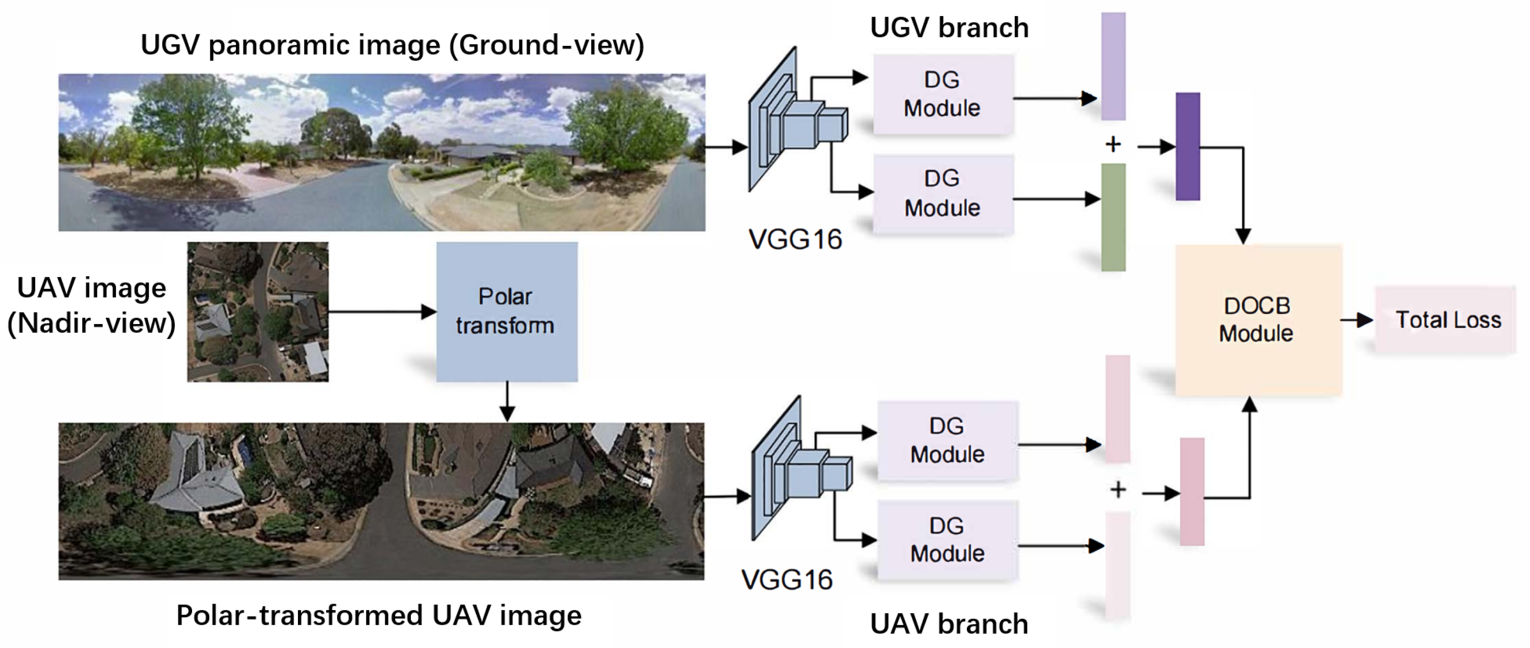
In this section, the network architecture of the proposed MSFA is illustrated first. Like some recent works [29,34], we adopt a two-branch Pseudo-Siamese structure (without sharing weights), as depicted in Figure 2. Then, the details of the Dynamic Online Cross-Batch (DOCB) hard exemplar mining module are introduced.

3.1. Overview

In this paper, we propose a progressive and efficient cross-batch hard exemplar mining strategy consisting of two phases. In the first phase, we perform hard exemplar mining only within the batch until the network converges, which prepares for the second phase of hard exemplar mining across batches. In the second phase, we store the descriptors generated by the previous batches’ exemplars in a queue and select the hardest hard exemplar for each anchor in the current batch to calculate the triplet loss. Furthermore, we propose a novel Siamese network architecture MSFA that refines multi-scale features separately, selects the most valuable information, and fuses the features to obtain the final descriptor. The overall network pipeline is illustrated in Figure 2.

3.2. Network Architecture

The proposed multi-scale feature aggregation (MSFA) network focuses on extracting discriminative features by compressing features from two different scales and fusing related parts of the features to pay more attention to local details. The network gives a smart change to the backbone of VGG16. Specifically, it obtains two groups of feature maps from the last two blocks of VGG16, denoted as $F_{block4}$ and $F_{block5}$. $F_{block4}$ becomes the same size as $F_{block5}$ after $2\times 2$ pooling. Then, $F_{block4}$ and $F_{block5}$ are separately sent to two DG (Descriptor Generator) modules which do not share weights.

The structure of the DG module is also very simple, consisting of $2\times 2$ pooling, $3\times 3$ convolution, and $1\times 1$ convolution. The DG module is similar to VGG16 in style. The pooling is designed to decrease the feature dimension and the length of descriptors. The $3\times 3$ convolution captures local context information about feature maps. Due to the redundancy in the channel information regarding convolutions, we use $1\times 1$ convolutions to select the eight most valuable channels. Subsequently, we fuse the eight-channel feature maps obtained from the output of the DG modules of two different scales and flatten them to obtain the final descriptor. Compared with different fusion strategies, the sum operation is finally adopted as our fusion method. The fusion of descriptors from two scales greatly improves the performance of our network. The effect can be seen in Section 4.8.2.

3.3. Dynamic Online Cross-Batch Hard Exemplar Mining Scheme

The proposed Dynamic Online Cross-Batch (DOCB) Hard Exemplar Mining Scheme is a scheme for hard exemplar mining in the cross-view geo-localization task. It consists of two phases. In the first phase, hard exemplar mining is performed within the mini-batch. In the second phase, the descriptors generated in previous mini-batches’ exemplars are stored in a queue, and the hardest hard exemplar for each anchor in the current mini-batch is selected to calculate the triplet loss. This scheme can make the mining range of hard exemplars almost independent of batch size.

The key advantage of the DOCB is that it enables the network to mine hard negative exemplars from previous mini-batches and incorporate their gradient into training. This process assists the triplet loss in more effectively guiding the network to learn valuable metric information. In the cross-view geo-localization task, where each class (location) has only two images (ground-view and nadir-view), hard negative exemplar mining is particularly necessary. By utilizing the DOCB, the network can mine hard negative exemplars across mini-batches, which is not possible with traditional triplet sampling methods that are limited to the mini-batch range. The Dynamic Online Cross-Batch (DOCB) Hard Exemplar Mining module consisting of two phases is illustrated in Figure 3.

The formula for the total loss of our DOCB is as follows:

$$Los{s}_{total}=Los{s}_{intra}+Los{s}_{cross}$$

(1)

where $Los{s}_{intra}$ is the intra-batch hard exemplar mining loss, and $Los{s}_{cross}$ is the cross-batch hard exemplar mining loss. Both $Los{s}_{intra}$ and $Los{s}_{cross}$ are weighted soft margin triplet losses [21]. The original weighted soft margin triplet loss can be expressed as follows:

$$Los{s}_{triplet}=ln(1+exp\left(\alpha (d^p(a_i,p_i)-d^n(a_i,n_k))\right))$$

(2)

We adopt the exhaustive mini-batch scheme [19] to increase the number of available triplets in a mini-batch, resulting in $2\times B\times (B-1)$ (B is the batch size) triplet pairs. Here, $\alpha$ is a scaling coefficient, $d^n(a_i,n_k)$ is the Euclidean distance between the negative pair, and $d^p(a_i,p_i)$ is the distance between the positive pair.

At the beginning, we only calculate $Los{s}_{intra}$, without computing $Los{s}_{cross}$. This setup can make the training smoother, since mining the hardest exemplar at the beginning of the training will make the training difficult to converge.

In the process of computing $Los{s}_{intra}$, triplets that have a $\varphi$ value greater than the threshold $\beta =0.15$ are deemed too easy and are discarded. These triplets have already effectively distinguished the positive and negative pairs, rendering further gradient calculations unnecessary. Therefore, we directly discard them to ensure that the loss of the truly hard triplets is not diluted. However, a potential issue with this approach arises as the training progresses. It is possible for all loss values within the current mini-batch to rise above the $\beta$ threshold. In such cases, we calculate the top 1 hard triplet loss to replace $Los{s}_{intra}$, which only computes the loss for the hardest triplet within the current mini-batch. $Los{s}_{intra}$ is represented as Equation (3).

$$Los{s}_{intra}={\displaystyle \frac{1}{2N}}\sum _{i=1}^B\sum _{\begin{array}{c}k=1\\ k!=i\\ \varphi (i,k)<\beta \end{array}}^{B}ln(1+exp(-\alpha \varphi (i,k)))$$

(3)

where $\varphi (i,k)=d^n(a_i,n_k)-d^p(a_i,p_i)$ is the difference between the distances of the anchor-positive pairs and anchor-negative pairs. And N represents the number of effective triplets with $\varphi (i,k)$ less than $\beta$.

When computing $Los{s}_{cross}$, a queue named “memory bank” is maintained to store the descriptors of negative exemplars generated in previous mini-batches. Then, the similarity is calculated between the descriptors of anchor exemplars in the current mini-batch and negative exemplars in “memory bank”. On this basis, for each anchor in the current mini-batch, the negative exemplar with the highest similarity to it is selected from the queue as the hardest exemplar. This exemplar is then paired with the anchor and the corresponding positive exemplar to form a cross-batch triplet, which is reloaded into the network by its label, and its gradient can be computed.

The form of $Los{s}_{cross}$ is given by Equation (4). Here, Q represents the “memory bank” queue that stores the descriptors of previous mini-batches, B is the batch size, and $n_j$ is the negative exemplar from Q. The length of the queue is $M\times B$, where M is the maximum number of mini-batches that the queue can store. It is important to note that the mined negative exemplars need to be reloaded into the network before computing $Los{s}_{cross}$.

$$Los{s}_{cross}={\displaystyle \frac{1}{2B}}\sum _{i=1}^{B}ln(1+exp(\alpha (d^p(a_i,p_i)-\underset{n_j\in Q}{min}{d}^n(a_i,n_j))))$$

(4)

The “memory bank” is updated as follows: First, the descriptors of the current mini-batch exemplars are pushed into the queue. Then, the similarity between anchor exemplars in the current mini-batch and negative exemplars from the previous mini-batches in the current queue is calculated. After that, the negative exemplar with the largest similarity is selected as the hardest exemplar for each anchor in the current mini-batch to compute $Los{s}_{cross}$. It is important to note that the new descriptors of the hard exemplars generated by the network after reloading are restored in the queue. This speeds up the updating of our memory bank queue, ensuring that the exemplar descriptors in the queue remain as up-to-date as possible. Finally, when the queue is full, the oldest descriptors are dequeued.

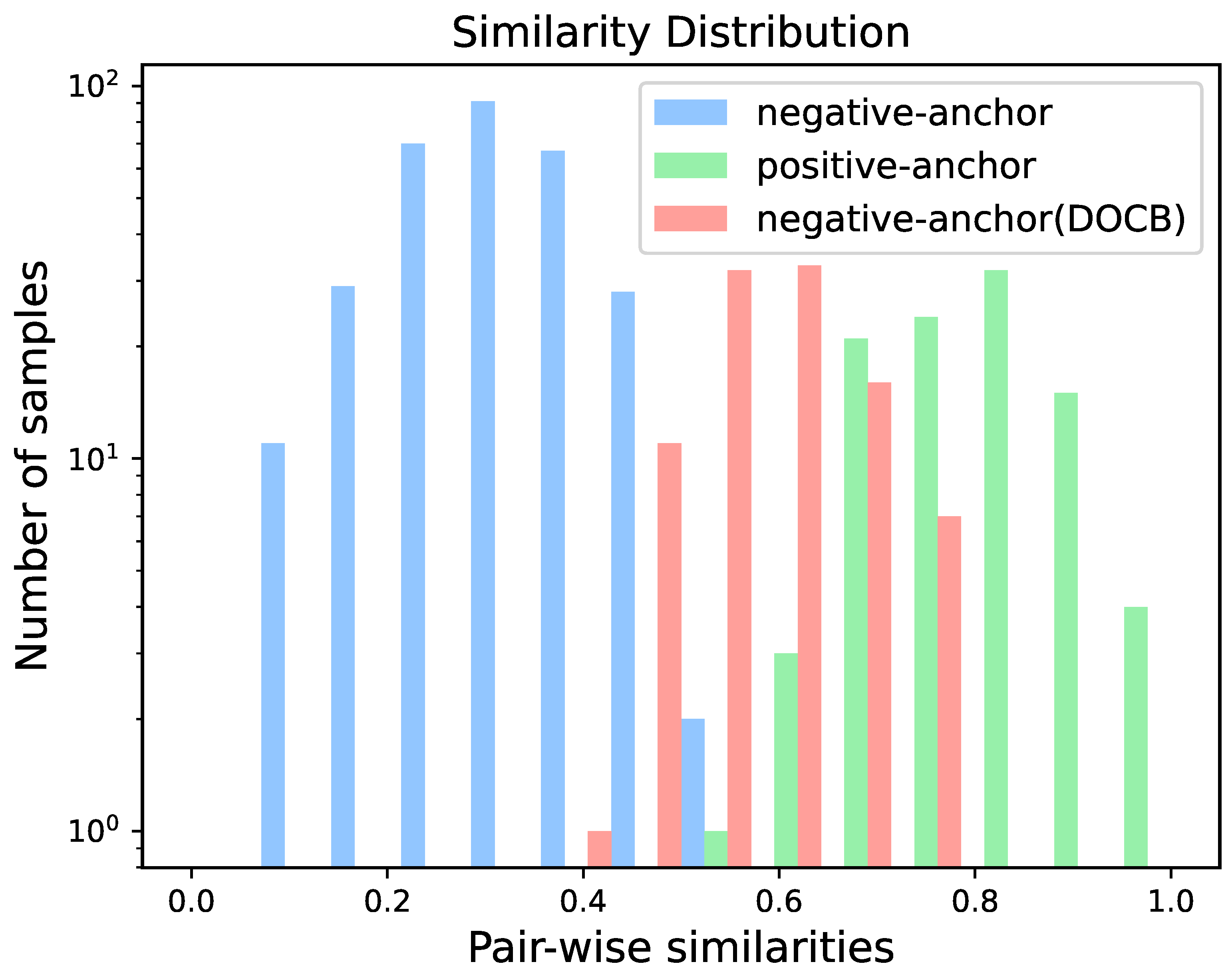
To visually and intuitively demonstrate the role of the DOCB, we randomly selected a mini-batch from the first epoch when $Los{s}_{cross}$ values were computed and mined the hardest negative exemplar by the DOCB for each anchor. Figure 4 shows the similarity distribution of triplets in this mini-batch and the triplets mined by our DOCB. It can be seen that negative pairs in a mini-batch have already been distinguished from the positive pairs by similarity metrics. However, the similarity of the anchors and the cross-batch negative pairs mined by the DOCB is much closer to that of the positive pairs. Therefore, these hard exemplars mined by the DOCB are more valuable for network training to learn more distinguishable metric information.

4. Experiments

4.1. Datasets

The experiments are conducted on two benchmark datasets, CVUSA [35] and CVACT [2], which exhibit a basic level of center alignment between the centers of nadir-view (UAV or satellite) and ground-view (UGV) images. In the upcoming sections, we will proceed to introduce each of these datasets individually.

4.1.1. CVUSA

CVUSA stands as an early large-scale cross-view geo-localization dataset, collected from various regions within the United States. The dataset contains 35,532 pairs of satellite nadir-view and ground-level UGV images (street-view) for training, along with an additional 8884 pairs reserved for evaluation. The original dimensions of the satellite images are 750 × 750 pixels, while the panoramic street-view images measure 224 × 1232 pixels. Notably, each image pair was meticulously collected with stringent center alignment considerations, ensuring that the northern orientation of the satellite image aligns with the central axis of the panoramic street-view image.

4.1.2. CVACT

The CVACT dataset maintains a consistent configuration in terms of the number of samples in both its training and testing sets while also furnishing an extensive test set encompassing 92,802 pairs of images. Notably, CVACT exclusively collects data from the city of Canberra, Australia. This dataset presents a distinct feature of higher resolution for both satellite images and street-view images. The satellite images within CVACT possess dimensions of 1200 × 1200 pixels, while the street-view images measure 832 × 1664 pixels.

4.2. Evaluation Protocol

To evaluate the performance of our method and the compared algorithms, we adopt the recall at top 1, top 5, and top 1% as evaluation metrics. These are rank-based evaluation metrics widely used in image retrieval.

4.3. Implementation Details

The nadir-view images are polar-transformed and resized to $128\times 512$ pixels along with the corresponding ground images as the input. The VGG16 (excluding full connection layer) pre-trained on Imagenet [36] is used as our backbone to extract features. The scaling coefficient [21] $\alpha$ is set to 10.0, and the value of $\beta$ is set to 0.15 in accordance with the experimental setup described in [9]. To maximize the number of triplets within each mini-batch, we use an exhaustive mini-batch scheme [19]. We train our network using the AdamW [37] optimizer with a learning rate of 1 × ${10}^{-5}$ and a weight decay of 3 × ${10}^{-2}$ for 300 epochs and start computing $Los{s}_{cross}$ from the 250th epoch. In order to ensure a fair comparison with other approaches, we set the batch size to 32 in all experiments. The impact of M is analyzed in Section 4.8.4.

4.4. A Comparison with the State of the Art

We conducted a comparative evaluation of our proposed method with several state-of-the-art approaches in the field of cross-view geo-localization on both the CVUSA and CVACT datasets.

Table 1. A performance comparison with SOTA methods on the CVUSA dataset and CVACT dataset. (PT) means that polar transformation was used. The highest and second highest recall rates are marked in red and blue, respectively.

Model	CVUSA			CVACT_Val			CVACT_Test
	r@1	r@5	r@1%	r@1	r@5	r@1%	r@1	r@5	r@1%
CVM-Net [21]	22.47	49.98	89.62	20.15	45.00	87.57	5.41	14.79	54.53
Liu and Li [2]	40.79	66.82	96.12	46.96	68.28	92.01	19.21	35.97	60.69
CVFT [1]	61.43	84.69	99.02	61.05	81.33	95.93	26.12	45.33	71.69
LPN (PT)  [38]	85.79	95.38	99.41	79.99	90.63	97.03	-	-	-
SAFA + LPN (PT)  [38]	92.83	98.00	99.78	83.66	94.14	98.41	-	-	-
SAFA (PT)  [3]	89.84	96.93	99.64	81.03	92.8	98.17	55.50	79.94	94.49
SAFA + 4SCIG [43]	92.91	98.15	99.79	83.18	93.35	99.30	-	-	-
DSM (PT)  [22]	91.96	97.50	99.67	82.49	92.44	97.32	35.63	60.07	84.75
CDE (PT)  [41]	92.56	97.55	99.57	83.28	93.57	98.22	61.29	85.13	98.32
LPN + USAM (PT)  [40]	91.22	-	99.67	82.02	-	98.18	-	-	-
L2LTR (PT)  [4]	94.05	98.27	99.67	84.89	94.59	98.37	60.72	85.85	96.12
L2LTR + 4SCIG [43]	93.82	98.62	99.70	81.54	93.11	97.95	-	-	-
TransGeo [6]	94.08	98.36	99.04	-	-	-	-	-	-
TransGeo + 4SCIG [43]	91.10	98.74	99.81	83.73	94.41	98.41	-	-	-
TransGCNN (PT)  [5]	94.15	98.21	99.79	84.92	94.46	98.36	-	-	-
DeHi [30]	94.34	98.63	99.82	84.96	94.48	98.58	-	-	-
MSFA (PT) (Ours)	94.38	98.32	99.71	85.53	94.39	98.37	63.04	86.12	96.10
MSFA (PT) + DOCB (Ours)	95.78	98.50	99.67	86.34	94.42	98.24	63.90	86.95	95.99

summarizes the performance comparison results. The compared methods include the convolutional network CVM-Net [21], Liu and Li [2], LPN [38], CVFT [1], DSM [22], SSA-Net [39], USAM [40], and CDE [41]. In addition, we compared our approach with three transformer-based networks, namely L2LTR [42], TransGCNN [5], and TransGeo [6]. $MSFA$ in the above table adopts the original weighted soft margin triplet loss [21] without any hard exemplar mining. $MSFA+DOCB$ refers to the proposed network with hard exemplar mining module DOCB.

The results show that $MSFA$ significantly outperforms all previous CNN-based methods using polar transformation (PT) on both datasets. Meanwhile, L2LTR, TransGCNN, and TransGeo achieve similar performance to $MSFA$ without using polar transformation (PT) on the CVUSA dataset, benefiting from learnable position encoding and a stronger transformer-based backbone than VGG16. This indicates that transformer can learn the geometric correspondence of two different views by explicit position encoding and long-range correlation of multi-head attention. Meanwhile, $MSFA+DOCB$ achieves better top 1 recall performance than previous CNN-based methods and transformer-based methods on the CVACT dataset. Note that with/without $DOCB$, our model can achieve a top 1 recall of 63.90% and 63.04% on CVACT_test, respectively, while the transformer-based model L2LTR(PT) only achieves 60.72%.

4.5. Comparison with Other Hard Exemplar Mining Methods

We compared our cross-batch hard exemplar mining scheme with three other existing works: SEH loss [9], Global mining [8], and XBM [10].

Table 2. Comparison with other hard exemplar mining methods on CVUSA dataset. The highest and second highest recall rates are marked in red and blue, respectively.

Method	Batch Size	r@1
DSM [22] + SEH [9]	30	94.46
DSM [22] + SEH [9]	90	94.91
DSM [22] + SEH [9]	120	95.11
DSM [22] + DOCB	32	95.02
MSFA + XBM-hard	32	94.90
MSFA + Global mining [8]	32	94.74
MSFA + DOCB (Ours)	32	95.78

shows the accuracy of three different hard exemplar mining methods on the CVUSA dataset. The SEH loss is based on the DSM backbone network, so we also used our DOCB on DSM. It can be seen that although our batch size is always 32, the performance is similar to that of the DSM method with a batch size of 120, and it outperforms other methods in terms of SEH loss on other smaller batch sizes.

In addition, we compared the Global mining method with our DOCB method on the proposed network, MSFA. It can be seen that our method outperforms Global mining, with a top 1 recall rate improvement of around 1%.

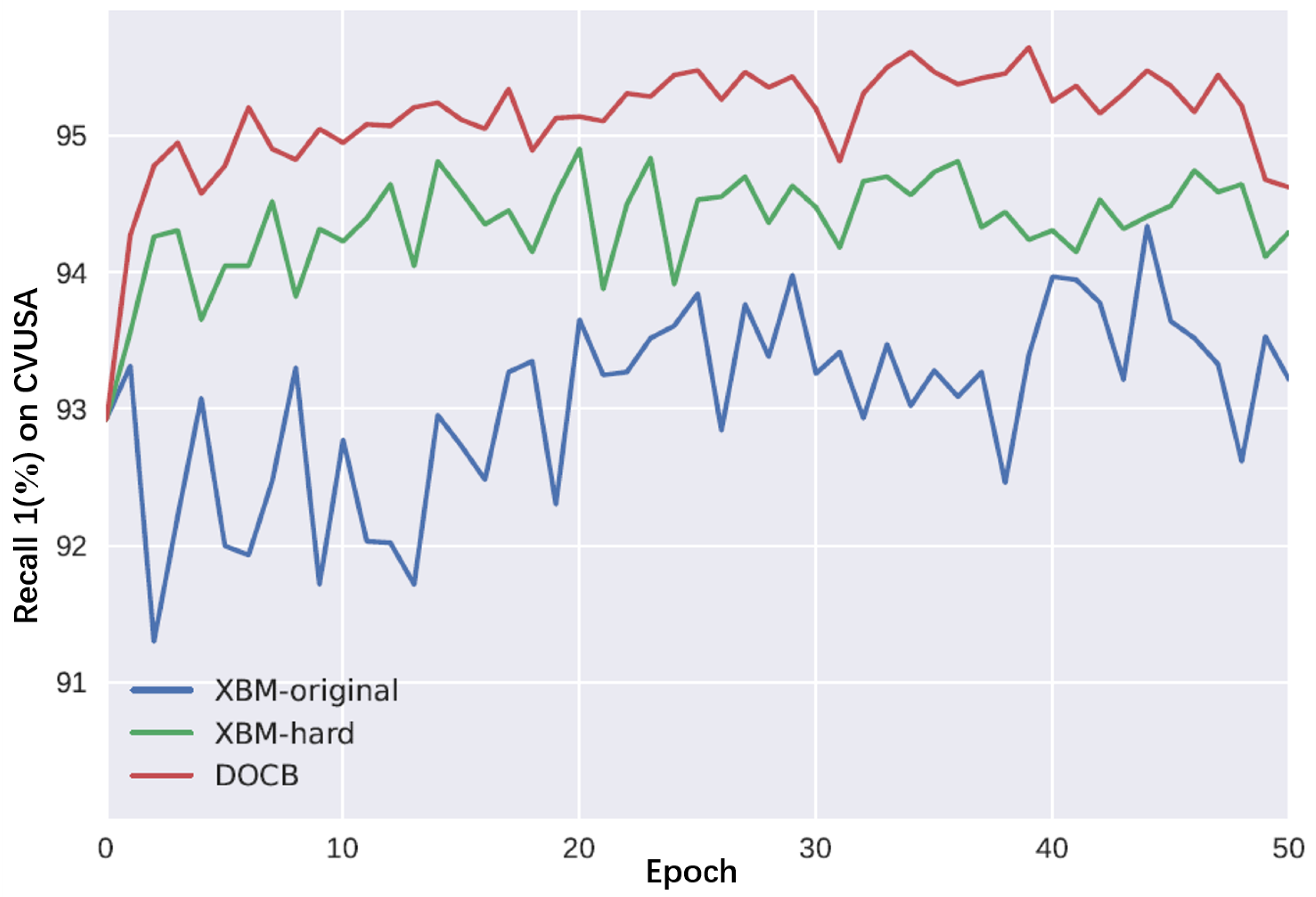
Finally, we compared our method with the most similar XBM method. Since the original XBM method performed poorly on CVUSA and CVACT, we used our improved top 1 hard version of XBM named XBM-hard. The only difference between our DOCB method and XBM-hard is that XBM-hard directly calculates the top 1 hard triplet loss using descriptors from the queue, without reloading them into the network.

It can be seen that our method is significantly better than XBM-hard. Also, Figure 5 shows the recall rate curves of DOCB, XBM-hard, and the original version of XBM (XBM-original).

4.6. Computational Cost

To evaluate the efficiency of our proposed method, an extra comparison experiment is conducted on the CVUSA dataset, shown in

Table 3. Computational cost comparison on CVUSA dataset. Inference Time (Per Batch) is tested on same GTX 2080 Ti with batch size of 32 for all methods. Note that TransGeo adopts additional acceleration strategy. The highest and second highest recall rates are marked in red and blue, respectively.

Model	Param (M)	GFLOPs	Inference Time (Batch) (ms)	r@1
SAFA [3]	29.50	42.24	110	89.84
DSM [22]	17.90	-	-	91.96
L2LTR [4]	195.90	-	-	94.05
TransGCNN [5]	87.80	-	-	94.15
TransGeo [6]	44.8	11.32	99	94.08
MSFA (Ours)	38.90	40.68	108	94.38
MSFA + DOCB (Ours)	38.90	40.68	108	95.39

. The number of parameters (Param), GFLOPs, Inference Time (Per Batch), and the top 1 recall (r@1) are adopted as the evaluation criteria. It can be seen that our network not only achieves the highest accuracy, but it also has fewer parameters and a faster inference speed. Note that TransGeo is slightly faster than our method, but it adopts an additional acceleration scheme.

While the proposed DOCB mechanism introduces additional computational overhead during training—primarily from maintaining the dynamic FIFO queue and calculating cross-batch similarities—it is critical to emphasize that this cost is confined to the training phase. The DOCB module is inactive during inference; thus the final model’s GFLOPs and inference latency remain competitive with the baseline methods, as shown in Table 3. We posit that the incurred training cost is a worthwhile trade-off for obtaining a model with significantly enhanced representation power without compromising inference efficiency.

4.7. Descriptor Length Comparison Experiment

In image retrieval, shorter encoding lengths of image descriptors lead to lower storage costs of the reference database and faster matching speeds.

Table 4. A comparison of descriptor length. The highest and second highest recall rates are marked in red and blue, respectively.

Model	Descriptor Length	r@1
SAFA [3]	4096	89.84
DSM [22]	4096	91.96
L2LTR [4]	768	94.05
TransGeo [6]	1000	94.08
MSFA (Ours)	512	94.38

shows the descriptor lengths of state-of-the-art methods and their corresponding top 1 recall rates on the CVUSA dataset. Our proposed approach achieves better performance than other methods while using a shorter descriptor length.

4.8. Ablation Experiments

In this section, to verify the effectiveness of sub-modules in our entire framework, we conduct ablation experiments on the DG module, feature fusion method, and the DOCB. Meanwhile, we also test and compare different M values to analyze their impacts on the CVUSA and CVACT_val datasets.

4.8.1. Effect of DG Module

To verify the effect of our DG module, we designed two networks, namely $VG{G}_{gp}$ and $MSF{A}_{Single}$. The $MSF{A}_{Single}$ model extracts features from the last block of VGG16 and then passes through a DG module to generate the image descriptor. Compared with our $MSFA$, the $MSF{A}_{Single}$ model only considers the global descriptor $D_{global}$ and disregards multi-scale fusion, because we only want to evaluate the DG module. The $VG{G}_{gp}$ model is similar to $MSF{A}_{Single}$; the only difference is that it adopts global pooling instead of the DG module. SAFA is also similar, but it adopts spatial-aware feature aggregation instead of the DG module.

Table 5. Effectiveness demonstration of Descriptor Generator module on CVUSA dataset. The highest and second highest recall rates are marked in red and blue, respectively.

Model	r@1 (%)
$VG{G}_{gp}$	65.74
$SAFA$	89.84
$MSF{A}_{Single}$	93.29

shows the comparison results of these three networks. It can be seen that $MSF{A}_{Single}$ has much better performance by using the DG module than the others.

4.8.2. Effect of Fusion Strategy

To verify the effectiveness of fusion and compare different fusion methods, we evaluated five approaches: $MSF{A}_{single}$, $MSF{A}_{concat}$, $MSF{A}_{sum3}$, $MSF{A}_{sk}$, and $MSFA$. We only extract features from the last block of VGG and then use our DG module without fusion features to remove the influence of the fusion method, which is denoted as $MSF{A}_{single}$. $MSF{A}_{concat}$ is similar to $MSFA$, but it uses concatenation as the fusion operation. $MSF{A}_{sum3}$ extracts feature maps from the last three blocks of VGG16, downsamples them to the same size, applies different DG modules separately, and finally performs summation fusion to generate the final image descriptor. Following the fusion method in SKnet [44], we also apply attention modules on the outputs of blocks 4 and 5 and then fuse them by summing, denoted as $MSF{A}_{sk}$. As shown in

Table 6. Effectiveness of fusion scheme on CVUSA dataset. The highest and second highest recall rates are marked in red and blue, respectively.

Model	Fusion Strategy	r@1
$MSF{A}_{single}$	none	93.29
$MSF{A}_{concat}$	concatenate	93.82
$MSF{A}_{sum3}$	summation	93.92
$MSF{A}_{sk}$	attention + summation	94.12
$MSFA$	summation	94.38

, compared to $MSF{A}_{single}$, the other three fusion methods achieved higher top 1 recall, thanks to the fusion of feature maps of different scales. Compared with $MSFA$ and $MSF{A}_{sum3}$, the accuracy of $MSF{A}_{concat}$ is slightly lower. We conclude that the summation fusion scheme is more suitable for our network than concatenation. The performance of $MSFA$ is slightly better than that of $MSF{A}_{sum3}$, indicating that the features from the last two layers of VGG16 are sufficient to describe the input image. Our method achieves slightly higher performance than $MSF{A}_{sk}$ without extra attention computation.

4.8.3. Effectiveness of DOCB

In this section, we conducted ablation experiments by removing $Los{s}_{intra}$, $Los{s}_{cross}$, and $DOCB$ to analyze the their impact on the framework. The results are shown in the following

Table 7. Effectiveness of DOCB on CVUSA dataset. The highest and second highest recall rates are marked in red and blue, respectively.

Method	Batch Size	r@1
$MSFA+None$	32	94.38
$MSFA+Los{s}_{intra}$	32	94.52
$MSFA+Los{s}_{cross}$	32	95.41
$MSFA+DOCB$	32	95.78

. $Los{s}_{intra}$ means that only $Los{s}_{intra}$ is used for training, without using $Los{s}_{cross}$, and $Los{s}_{cross}$ means that a regular soft margin triplet loss is used without intra-batch hard exemplar mining to replace $Los{s}_{intra}$, but $Los{s}_{cross}$ is calculated in the same way as $DOCB$. Finally, a represents the baseline where no hard exemplar mining is used. Overall, the $Los{s}_{cross}$ part has a more significant impact on the performance compared to the $Los{s}_{intra}$ part. However, removing the $Los{s}_{intra}$ part results in a significant drop in the final performance, indicating that our cross-batch hard exemplar mining requires the preceding intra-batch hard exemplar mining as a prerequisite to some extent. At the same time, it does not entirely rely on hard exemplar mining within the mini-batch. We were still able to achieve a top 1 recall rate of 95.41% on the CVUSA dataset even when removing the intra-batch mining loss.

4.8.4. Effectiveness of Hyper-Parameter M

The length of the queue of the memory bank is $M\times B$ (batch size). The choice of M is crucial, as it can influence the level of difficulty of the mined hard exemplars. A queue that is too short may not yield effective hard exemplars, while one that is too long may lead to overly hard exemplars and thus poor performance. We conducted an experiment to investigate the impact of M on both CVUSA and CVACT_val datasets, and

Table 8. The influence of hyper-parameter M in our DOCB. The highest and second highest recall rates are marked in red and blue, respectively.

Dataset	M	r@1 (${\mathit{Loss}}_{\mathit{intra}}$)	r@1
	20		95.12
CVUSA	200	93.82	95.46
	1000		95.78
	20		86.34
CVACT_val	200	85.15	86.26
	1000		85.22

presents the corresponding results for several typical values of M (1000, 200, and 20). Based on the experiment results, we set M to 1000 for CVUSA and 20 for CVACT. Here, $r@1\left(Los{s}_{intra}\right)$ denotes the highest top 1 recall before computing $Los{s}_{cross}$.

4.9. The Effect of Multi-Scale Aggregation and the Parallel Operation

To individually analyze and explore the impact of multi-scale aggregation and the parallel operation of the two DG (Depthwise Convolutional) modules, we conducted comparative experiments on the CVUSA dataset. Firstly, we performed multi-scale aggregation by adding the features from the fourth and fifth blocks of VGG16, followed by a single DG module, denoted as $MSFA-ms$. Subsequently, we appended the two parallel DG modules to the end of the fifth block of VGG16 without performing multi-scale fusion, referred to as $MSFA-nms$. The experimental results are presented in

Table 9. The effect of multi-scale aggregation and the parallel operation. The highest and second highest recall rates are marked in red and blue, respectively.

Model	Multi-Scale	Parallel	r@1
$MSF{A}_{single}$	No	No	93.29
$MSF{A}_{ms}$	Yes	No	94.02
$MSF{A}_{nms}$	No	Yes	93.81
$MSFA$	Yes	Yes	94.38

.

4.10. Cross-Dataset Transferring Performance

When applying a model to real geo-location scenarios, the input images are often very different from those in the training set. Therefore, transferring ability is very important. We train our MSFA on the CVUSA dataset and test it on CVACT_val and denote it as CVUSA → CVACT and vice versa. Then, we compare these two with some state-of-the-art studies which also conducted transferring experiments and reported their performance, shown in

Table 10. Cross-dataset transferring performance comparison with state-of-the-art methods. The highest and second highest recall rates are marked in red and blue, respectively.

Task	Model	r@1	r@5	r@1%
CVUSA→CVACT	SAFA [3]	30.40	52.93	85.82
	DSM [22]	33.66	52.17	79.67
	L2LTR [4]	47.55	70.58	91.39
	MSFA (Ours)	53.67	75.02	93.26
CVACT→CVUSA	SAFA [3]	21.45	36.55	69.83
	DSM [22]	18.47	34.46	69.01
	L2LTR [4]	33.00	51.87	84.79
	MSFA (Ours)	44.17	63.47	89.33

. It can be seen that our model has better transferring ability than the others, including transformer-based model L2LTR.

4.11. Visualization of Retrieval Results

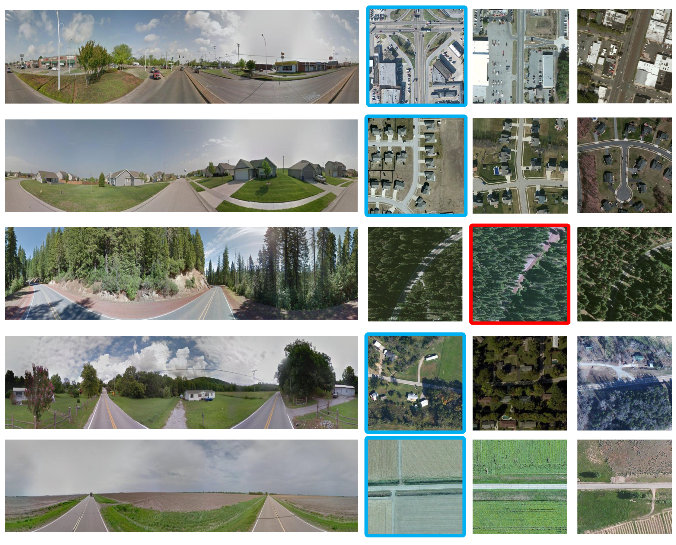
We present several typical retrieval results of our model on the CVUSA dataset in Figure 6, including four correct retrieval examples and one incorrect retrieval example. Our method can accurately pick out the correct image from many similar candidates and performs well in various scenarios, such as urban areas (row 1 and row 2), rural areas (row 4), and suburban areas (row 5). It is noteworthy that although the top 1 and top 2 satellite images (nadir-view) in row 5 are very similar, our model can still discriminate between them, which proves that our network can effectively encode local details. However, due to the look-down viewpoint of satellites, satellite images with dense towering trees often face the problem of occlusion, where the ground targets are partially or entirely obscured. Our method fails in the third example due to the influence of occlusion in the satellite image.

5. Conclusions

In this paper, we present a novel dynamic online scheme for mining hard cross-batch exemplars. Our approach involves maintaining a dynamic FIFO queue to store generated descriptors, and unlike previous epoch-based offline cross-batch mining methods, our approach calculates the similarity between the current mini-batch exemplar descriptors and the descriptors in the queue on each iteration. This allows us to effectively mine the hardest cross-batch negative exemplar for each anchor and reload them into the network to correct the gradient of the negative exemplars. This scheme effectively addresses the problem of network stagnation due to the lack of hard exemplars at the later stage of training. In addition, we also propose a Siamese network that can integrate multiple local spatial features to obtain multi-scale feature aggregation, enabling the network to pay attention to detailed information. Finally, our proposed DOCB and MSFA outperform all existing methods on two benchmark datasets, CVUSA and CVACT_val with the shortest descriptor length and the best cross-dataset transferability.

References

1. Shi, Y.; Yu, X.; Liu, L.; Zhang, T.; Li, H. Optimal feature transport for cross-view image geo-localization. In Proceedings of the AAAI Conference on Artificial Intelligence, New York, NY, USA, 7–12 February 2020; Volume 34, pp. 11990–11997. [Google Scholar]
2. Liu, L.; Li, H. Lending orientation to neural networks for cross-view geo-localization. In Proceedings of the IEEE/CVF Conference on Computer Vision and Pattern Recognition, Long Beach, CA, USA, 15–20 June 2019; pp. 5624–5633. [Google Scholar]
3. Shi, Y.; Liu, L.; Yu, X.; Li, H. Spatial-aware feature aggregation for image based cross-view geo-localization. Adv. Neural Inf. Process. Syst. 2019, 32, 1–11. [Google Scholar]
4. Yang, H.; Lu, X.; Zhu, Y. Cross-view geo-localization with layer-to-layer transformer. Adv. Neural Inf. Process. Syst. 2021, 34, 29009–29020. [Google Scholar]
5. Wang, T.; Fan, S.; Liu, D.; Sun, C. Transformer-guided convolutional neural network for cross-view geolocalization. arXiv 2022, arXiv:2204.09967. [Google Scholar]
6. Zhu, S.; Shah, M.; Chen, C. Transgeo: Transformer is all you need for cross-view image geo-localization. In Proceedings of the IEEE/CVF Conference on Computer Vision and Pattern Recognition, New Orleans, LA, USA, 18–24 June 2022; pp. 1162–1171. [Google Scholar]
7. Cai, S.; Guo, Y.; Khan, S.; Hu, J.; Wen, G. Ground-to-aerial image geo-localization with a hard exemplar reweighting triplet loss. In Proceedings of the IEEE/CVF International Conference on Computer Vision, Seoul, Republic of Korea, 27 October–2 November 2019; pp. 8391–8400. [Google Scholar]
8. Zhu, S.; Yang, T.; Chen, C. Revisiting street-to-aerial view image geo-localization and orientation estimation. In Proceedings of the IEEE/CVF Winter Conference on Applications of Computer Vision, Virtual, 5–9 January 2021; pp. 756–765. [Google Scholar]
9. Guo, Y.; Choi, M.; Li, K.; Boussaid, F.; Bennamoun, M. Soft exemplar highlighting for cross-view image-based geo-localization. IEEE Trans. Image Process. 2022, 31, 2094–2105. [Google Scholar] [CrossRef]
10. Wang, X.; Zhang, H.; Huang, W.; Scott, M.R. Cross-batch memory for embedding learning. In Proceedings of the IEEE/CVF Conference on Computer Vision and Pattern Recognition, Seattle, WA, USA, 14–19 June 2020; pp. 6388–6397. [Google Scholar]
11. Tan, Z.; Liu, A.; Wan, J.; Liu, H.; Lei, Z.; Guo, G.; Li, S.Z. Cross-batch hard example mining with pseudo large batch for id vs. spot face recognition. IEEE Trans. Image Process. 2022, 31, 3224–3235. [Google Scholar] [CrossRef] [PubMed]
12. Lowe, D.G. Distinctive image features from scale-invariant keypoints. Int. J. Comput. Vis. 2004, 60, 91–110. [Google Scholar] [CrossRef]
13. Bay, H.; Tuytelaars, T.; Van Gool, L. Surf: Speeded up robust features. In Proceedings of the Computer Vision–ECCV 2006: 9th European Conference on Computer Vision, Graz, Austria, 7–13 May 2006; Proceedings, Part I 9. Springer: Berlin/Heidelberg, Germany, 2006; pp. 404–417. [Google Scholar]
14. Sivic, J.; Zisserman, A. Video Google: Efficient visual search of videos. In Toward Category-Level Object Recognition; Springer: Berlin/Heidelberg, Germany, 2006; pp. 127–144. [Google Scholar]
15. Vo, N.; Jacobs, N.; Hays, J. Revisiting im2gps in the deep learning era. In Proceedings of the IEEE International Conference on Computer Vision, Venice, Italy, 22–29 October 2017; pp. 2621–2630. [Google Scholar]
16. Torii, A.; Arandjelovic, R.; Sivic, J.; Okutomi, M.; Pajdla, T. 24/7 place recognition by view synthesis. In Proceedings of the IEEE Conference on Computer Vision and Pattern Recognition, Boston, MA, USA, 7–12 June 2015; pp. 1808–1817. [Google Scholar]
17. Workman, S.; Jacobs, N. On the location dependence of convolutional neural network features. In Proceedings of the IEEE Conference on Computer Vision and Pattern Recognition Workshops, Boston, MA, USA, 7–12 June 2015; pp. 70–78. [Google Scholar]
18. Zhou, B.; Lapedriza, A.; Khosla, A.; Oliva, A.; Torralba, A. Places: A 10 million image database for scene recognition. IEEE Trans. Pattern Anal. Mach. Intell. 2017, 40, 1452–1464. [Google Scholar] [CrossRef]
19. Vo, N.N.; Hays, J. Localizing and orienting street views using overhead imagery. In Proceedings of the European Conference on Computer Vision, Amsterdam, The Netherlands, 11–14 October 2016; Springer: Berlin/Heidelberg, Germany, 2016; pp. 494–509. [Google Scholar]
20. Arandjelovic, R.; Gronat, P.; Torii, A.; Pajdla, T.; Sivic, J. NetVLAD: CNN architecture for weakly supervised place recognition. In Proceedings of the IEEE Conference on Computer Vision and Pattern Recognition, Las Vegas, NV, USA, 27–30 June 2016; pp. 5297–5307. [Google Scholar]
21. Hu, S.; Feng, M.; Nguyen, R.M.; Lee, G.H. Cvm-net: Cross-view matching network for image-based ground-to-aerial geo-localization. In Proceedings of the IEEE Conference on Computer Vision and Pattern Recognition, Salt Lake City, UT, USA, 18–22 June 2018; pp. 7258–7267. [Google Scholar]
22. Shi, Y.; Yu, X.; Campbell, D.; Li, H. Where am i looking at? Joint location and orientation estimation by cross-view matching. In Proceedings of the IEEE/CVF Conference on Computer Vision and Pattern Recognition, Seattle, WA, USA, 14–19 June 2020; pp. 4064–4072. [Google Scholar]
23. Lu, X.; Luo, S.; Zhu, Y. It’s okay to be wrong: Cross-view geo-localization with step-adaptive iterative refinement. IEEE Trans. Geosci. Remote Sens. 2022, 60, 4709313. [Google Scholar] [CrossRef]
24. Sun, Y.; Ye, Y.; Kang, J.; Fernandez-Beltran, R.; Feng, S.; Li, X.; Luo, C.; Zhang, P.; Plaza, A. Cross-view object geo-localization in a local region with satellite imagery. IEEE Trans. Geosci. Remote Sens. 2023, 61, 4704716. [Google Scholar] [CrossRef]
25. Zheng, Z.; Wei, Y.; Yang, Y. University-1652: A multi-view multi-source benchmark for drone-based geo-localization. In Proceedings of the 28th ACM International Conference on Multimedia, Seattle, WA, USA, 12–16 October 2020; pp. 1395–1403. [Google Scholar]
26. Dai, M.; Hu, J.; Zhuang, J.; Zheng, E. A transformer-based feature segmentation and region alignment method for UAV-view geo-localization. IEEE Trans. Circuits Syst. Video Technol. 2021, 32, 4376–4389. [Google Scholar] [CrossRef]
27. Zhu, R.; Yang, M.; Yin, L.; Wu, F.; Yang, Y. UAV’s status is worth considering: A fusion representations matching method for geo-localization. Sensors 2023, 23, 720. [Google Scholar] [CrossRef] [PubMed]
28. Lv, H.; Zhu, H.; Zhu, R.; Wu, F.; Wang, C.; Cai, M.; Zhang, K. Direction-Guided Multi-Scale Feature Fusion Network for Geo-localization. IEEE Trans. Geosci. Remote Sens. 2024, 62, 5622813. [Google Scholar] [CrossRef]
29. Zhu, S.; Yang, T.; Chen, C. Vigor: Cross-view image geo-localization beyond one-to-one retrieval. In Proceedings of the IEEE/CVF Conference on Computer Vision and Pattern Recognition, Virtual, 19–25 June 2021; pp. 3640–3649. [Google Scholar]
30. Wang, T.; Li, J.; Sun, C. DeHi: A decoupled hierarchical architecture for unaligned ground-to-aerial geo-localization. IEEE Trans. Circuits Syst. Video Technol. 2023, 34, 1927–1940. [Google Scholar] [CrossRef]
31. Ge, F.; Zhang, Y.; Liu, Y.; Wang, G.; Coleman, S.; Kerr, D.; Wang, L. Multibranch joint representation learning based on information fusion strategy for cross-view geo-localization. IEEE Trans. Geosci. Remote Sens. 2024, 62, 5909516. [Google Scholar] [CrossRef]
32. Li, P.; Pan, P.; Liu, P.; Xu, M.; Yang, Y. Hierarchical temporal modeling with mutual distance matching for video based person re-identification. IEEE Trans. Circuits Syst. Video Technol. 2020, 31, 503–511. [Google Scholar] [CrossRef]
33. Duan, Y.; Lu, J.; Feng, J.; Zhou, J. Deep localized metric learning. IEEE Trans. Circuits Syst. Video Technol. 2017, 28, 2644–2656. [Google Scholar] [CrossRef]
34. Shi, Y.; Li, H. Beyond cross-view image retrieval: Highly accurate vehicle localization using satellite image. In Proceedings of the IEEE/CVF Conference on Computer Vision and Pattern Recognition, New Orleans, LA, USA, 18–24 June 2022; pp. 17010–17020. [Google Scholar]
35. Workman, S.; Souvenir, R.; Jacobs, N. Wide-area image geolocalization with aerial reference imagery. In Proceedings of the IEEE International Conference on Computer Vision, Santiago, Chile, 7–13 December 2015; pp. 3961–3969. [Google Scholar]
36. Deng, J.; Dong, W.; Socher, R.; Li, L.J.; Li, K.; Fei-Fei, L. Imagenet: A large-scale hierarchical image database. In Proceedings of the 2009 IEEE Conference on Computer Vision and Pattern Recognition, Miami, FL, USA, 20–25 June 2009; IEEE: Piscataway, NJ, USA, 2009; pp. 248–255. [Google Scholar]
37. Loshchilov, I.; Hutter, F. Decoupled weight decay regularization. arXiv 2017, arXiv:1711.05101. [Google Scholar]
38. Wang, T.; Zheng, Z.; Yan, C.; Zhang, J.; Sun, Y.; Zheng, B.; Yang, Y. Each part matters: Local patterns facilitate cross-view geo-localization. IEEE Trans. Circuits Syst. Video Technol. 2021, 32, 867–879. [Google Scholar] [CrossRef]
39. Zhang, X.; Meng, X.; Yin, H.; Wang, Y.; Yue, Y.; Xing, Y.; Zhang, Y. SSA-Net: Spatial scale attention network for image-based geo-localization. IEEE Geosci. Remote Sens. Lett. 2021, 19, 8022905. [Google Scholar] [CrossRef]
40. Lin, J.; Zheng, Z.; Zhong, Z.; Luo, Z.; Li, S.; Yang, Y.; Sebe, N. Joint representation learning and keypoint detection for cross-view geo-localization. IEEE Trans. Image Process. 2022, 31, 3780–3792. [Google Scholar] [CrossRef]
41. Toker, A.; Zhou, Q.; Maximov, M.; Leal-Taixé, L. Coming down to earth: Satellite-to-street view synthesis for geo-localization. In Proceedings of the IEEE/CVF Conference on Computer Vision and Pattern Recognition, Virtual, 19–25 June 2021; pp. 6488–6497. [Google Scholar]
42. Tian, Y.; Deng, X.; Zhu, Y.; Newsam, S. Cross-time and orientation-invariant overhead image geolocalization using deep local features. In Proceedings of the IEEE/CVF Winter Conference on Applications of Computer Vision, Snowmass Village, CO, USA, 1–5 March 2020; pp. 2512–2520. [Google Scholar]
43. Li, J.; Yang, C.; Qi, B.; Zhu, M.; Wu, N. 4scig: A four-branch framework to reduce the interference of sky area in cross-view image geo-localization. IEEE Trans. Geosci. Remote Sens. 2024, 62, 4703818. [Google Scholar] [CrossRef]
44. Li, X.; Wang, W.; Hu, X.; Yang, J. Selective kernel networks. In Proceedings of the IEEE/CVF Conference on Computer Vision and Pattern Recognition, Long Beach, CA, USA, 15–20 June 2019; pp. 510–519. [Google Scholar]
Figure 1. This figure illustrates the difference between XBM [10] (on the left) and DOCB (on the right) in terms of their respective mining strategies. In this figure, the blue point represents an anchor, the purple point represents its corresponding positive exemplar, and the dark red and light red points represent the same hard negative exemplar with past and current descriptors, respectively. The green arrows indicate the attraction between positive pairs, while the yellow arrows represent the repulsion between negative pairs. The dashed yellow arrow indicates the repulsion direction when using the past descriptor, and the purple arrow represents the shift caused by using the current descriptor. In our proposed DOCB, the repulsion direction is corrected to more accurately capture the relationships between the exemplars.
Ijgi 14 00418 g001
Figure 2. An overview of the proposed cross-view image-based geo-localization network. In our approach, the nadir-view UAV images undergo polar transformation [3] to align them with the ground-view UGV images before being jointly fed into the VGG16 network backbone. This process generates two distinct scale feature maps. Subsequently, these feature maps pass through two parallel Descriptor Generator (DG) modules, which enhance their representational capabilities. Following the DG modules, a fusion operation is applied to combine the outputs, resulting in the final multi-scale feature map. “+” represents the summation operation.
Ijgi 14 00418 g002
Figure 3. The structure of the DOCB, comprising two parts: intra-batch mining and cross-batch mining. The red lines represent the first phase, which includes the following: calculating similarity between each image pair (i), discarding easy triplets (ii), and finally computing L o s s i n t r a . The black lines represent the second phase, which includes the following: maintaining a FIFO queue to store image descriptors (iii), calculating similarity between the current mini-batch images and the descriptors in the queue to find negative exemplars (iv), reloading negative exemplars into the network to generate new descriptors (v), simultaneously updating these descriptors in the queue (vi), and finally computing L o s s c r o s s .
Ijgi 14 00418 g003
Figure 4. An example diagram of the similarity distribution of triplets. The green bars and the blue bars represent the positive pairs and the negative pairs in the current batch. The red bars represent cross-batch hard negative pairs mined by the DOCB.
Ijgi 14 00418 g004
Figure 5. A comparison of the DOCB and XBM [10]. The initial network state was the same. In this figure, “0” refers to the last epoch before cross-batch hard mining begins to be used. “XBM-hard” is a top 1 hard exemplar mining version of the XBM method, which mines the hardest negative exemplar for each anchor from a queue but does not reload it into the network.
Ijgi 14 00418 g005
Figure 6. The visualization of the retrieval results. From left to right are the ground images and the retrieved top 1 to top 3 satellite images (nadir-view). The red box indicates the failure of top 1 retrieval, and the blue box indicates the success of top 1 retrievals.
Ijgi 14 00418 g006