Article

STAE-BiSSSM: A Traffic Flow Forecasting Model with High Parameter Effectiveness

School of Electronic and Information Engineering, University of Science and Technology Liaoning, Anshan 114051, China
*
Author to whom correspondence should be addressed.
ISPRS Int. J. Geo-Inf. 2025, 14(10), 388; https://doi.org/10.3390/ijgi14100388
Submission received: 12 August 2025 / Revised: 29 September 2025 / Accepted: 30 September 2025 / Published: 4 October 2025

Abstract

Traffic flow forecasting plays a significant role in intelligent transportation systems (ITSs) and is instructive for traffic planning, management and control. Increasingly complex traffic conditions pose further challenges to the traffic flow forecasting. While improving the accuracy of model forecasting, the parameter effectiveness of the model is also an issue that cannot be ignored. In addition, existing traffic prediction models have failed to organically integrate data with well-designed model architectures. Therefore, to address the above two issues, we propose the STAE-BiSSSM model as a solution. STAE-BiSSSM consists of Spatio-Temporal Adaptive Embedding (STAE) and Bidirectional Selective State Space Model (BiSSSM), where STAE aims to process features to obtain richer spatio-temporal feature representations. BiSSSM is a novel structural design serving as an alternative to Transformer, capable of extracting patterns of traffic flow changes from both the forward and backward directions of time series with much fewer parameters. Comparative tests between baseline models and STAE-BiSSSM on five real-world datasets illustrates the advance performance of STAE-BiSSSM. This is especially so on METRLA and PeMSBAY datasets, compared with the SOTA model STAEformer. In the short-term forecasting task (horizon: 15 min), MAE, RMSE and MAPE of STAE-BiSSSM decrease by 1.89%/13.74%, 3.72%/16.19% and 1.46%/17.39%, respectively. In the long-term forecasting task (horizon: 60 min), MAE, RMSE and MAPE of STAE-BiSSSM decrease by 3.59%/13.83%, 7.26%/16.36% and 2.16%/15.65%, respectively.

1. Introduction

With the continuous development of urbanization, the number of vehicles has increased gradually [1], which has brought great pressure on the transportation system. The reduced efficiency of the transportation system directly leads to a series of phenomena, such as increased cost of transportation travel, frequent traffic congestion and a significant increase in the rate of traffic accidents and indirectly leads to a series of problems, such as energy waste, environmental pollution and economic losses. Geographic information science (GIS)-enabled intelligent transportation systems (ITSs), integrated with efficient and intelligent road health monitoring functions [2], are emerging as an effective solution to improve the traffic environment [3]. ITS can anticipate future traffic states by collecting and processing diverse historical data through smart infrastructure and advanced algorithms [4]. As a vital metric to measure traffic states, traffic flow reflects the traffic pressure on roads. Advanced path planning and traffic intervention based on traffic flow forecasting are efficient solutions to alleviate traffic congestion. Therefore, our proposed model STAE-BiSSSM is of practical significance.
In general, traffic forecasting models can be divided into three main categories including parametric techniques based models, machine learning techniques-based models and deep learning techniques-based models [5]. The representative models of parametric techniques based models include integrated autoregressive moving average (ARIMA)-based models [6,7,8] and kalman filters-based models [9,10,11], etc. The representative models of machine learning techniques-based models include support vector machine (SVM)-based models [12,13,14] and k-nearest neighbor (KNN)-based models [15], etc. However, parametric techniques-based models require prior knowledge and the construction of mathematical models in advance. Machine learning-based models lack the ability to process large-scale data. In recent years, the application of deep neural network in traffic forecasting has become a hot topic. This is because deep neural networks are characterized by high accuracy, strong nonlinear relationship processing ability, strong generalization ability, strong ability to deal with large-scale data, strong real-time forecasting and response and strong adaptability [16]. These deep learning models contain nonlinear autoregression with external input neural network (NARX), deep belief networks (DBNs), recurrent neural networks (RNNs), convolution neural networks (CNNs), graph neural networks (GNNs) and attention mechanisms [17]. Ref. [18] is a success application case for NARX for traffic flow forecasting combining data denoising. Ref. [19] is a representative example for DBN applied in traffic flow forecasting, which learns the features with limited prior knowledge. Subsequently, DBN have been overtaken by newer, more modern architectures, such as RNNs and CNNs. RNNs were first used to extract temporal features in traffic flow time series. Jordan network, a kind of RNN, was applied in [20,21]. The success of LSTM in NLP extends its application in traffic forecasting areas. For example, refs. [22,23,24,25] applied the LSTM and GRU for short-term traffic flow forecasting. Since traffic flow also have spatial properties, CNNs can be used to model the spatial relationship between roads. For example, models such as refs. [26,27,28,29,30,31,32,33] are structured by LSTM and CNN; GNN’s efficient processing of graph data makes it naturally suited to handle traffic flow forecasting tasks. For example, STGCN [34] is structured by CNN and GCN; models such as ref. [35,36,37,38,39], DCRNN [40] and TGCN [41] are characterized by novel graph convolution. Models such as AGCRN [42], GWNet [43], GTS [44], MTGNN [45] and Refs. [46,47] are able to learn graph structures to model more accurate, fine-grained spatial relationships between roads. Attention mechanism-based models become popular for their outstanding performance. For example, GMAN [48], PDFormer [49], AutoFormer [50], TrafficFormer [51] and MVSTT [52] are the representative models achieving the advanced performance. While more sophisticated and improved models are being designed to improve forecasting performance, attention is returning to the traffic data itself. For example, Shao et al. proposed STID [53] model which uses the one-hot encoding to integrate the spatial and temporal feature information into input data, thus enhances sample distinguishability. Liu et al proposed STAEformer [54] model which introduces a spatial–temporal adaptive embedding that enhances the capabilities of vanilla transformers for traffic flow forecasting.
Existing traffic flow forecasting models have not yet effectively addressed two key issues.
1.
Currently, mainstream traffic forecasting models are Transformer-based models. Quadratic computational complexity of attention mechanism results in a large number of parameters for this class of models, leading to high hardware requirements and high training cost, making model difficult deployment. Therefore, finding models with fewer parameters and excellent performance to replace Transformer has become a trend, such as RetNet [55], RWKV [56] and Mamba [57].
2.
There exists a disconnect in the optimization dimensions of current research efforts—some studies focus solely on improving the model’s network structure to enhance its fitting capability, while others concentrate exclusively on mining the features of traffic flow data. These two aspects fail to achieve organic integration, making it difficult to fully exert the synergistic effect of “structure adapting to data and data feeding back to structure”.
To address above issues, we propose the STAE-BiSSSM model, combining STAE and BiSSSM. BiSSSM is a newly designed model, and its core advantage lies in its ability to effectively capture the bidirectional dependencies of traffic flow from both the forward and backward direction of time series, thereby fully learning and modeling the dynamic evolution patterns of traffic flow. In addition, STAE enriches the representation of traffic flow feature, which significantly enhances the learning outcomes of BiSSSM. Compared with mainstream Transformer-based models, STAE-BiSSSM not only maintains performance advantages but also significantly reduces the number of model parameters, thus featuring higher efficiency. The main contributions of this paper are summarized as follows:
  • We designed a novel bidirectional selective state space model (BiSSSM) which is able to capture the bidirectional dependency of the traffic flow from both forward and backward direction of time series and better learn the dynamic change patterns of traffic flow.
  • We combined spatio-temporal adaptive embedding (STAE) and BiSSSM as a new model, STAE-BiSSSM, where STAE enriches the representation of traffic flow feature, thus enhancing the learning outcomes of BiSSSM.
  • STAE-BiSSSM shows the outstanding long- and short-term forecasting ability across five authoritative real-world datasets. In particular, on datasets METRLA and PeMSBAY, STAE-BiSSSM outperforms the SOTA model STAEformer.
  • Compared with STAEformer, STAE-BiSSSM has higher parameter effectiveness. While possessing superior performance, the number of trainable parameters of STAE-BiSSSM is much less than STAEformer.
The rest of this paper is organized as follows. Section 2 introduces the prerequisite knowledge and details of the STAE-BiSSSM model. In Section 3, we verify the effectiveness of the proposed model through a series of experiments. Finally, we conclude this paper in Section 4.

2. Methodology

2.1. Problem Definition

In this paper, we use the STAE-BiSSSM model to predict traffic flow over a certain time horizon based on historical traffic flow. Given traffic flow time series with l steps, we use X t l + 1 : t to infer the future l steps by training model F ( · ) with parameters θ , which can be formulated as:
X t + 1 , X t + 2 , , X t + l = F X t l + 1 , X t l + 2 , , X t ; θ
where traffic flow step is X i R n × d r a w and n is the number of spatial nodes. d r a w is the dimension of input feature.

2.2. Embedding Layer

The embedding layer contains three types of embedding which are feature embedding, periodicity embedding, and spatio-temporal adaptive embedding. In order to further enrich the feature representation of traffic flow while preserving the native information of the data. We utilize the fully connected layer to obtain feature embedding E f e a R l × n × d f e a :
E f e a = F C ( X t l + 1 : t )
where d f e a is the dimension of feature embedding and F C ( · ) indicates a fully connected layer. Since traffic is time-varying, labeling timestamps is critical. We denote the learnable timestamp-of-day embedding dict as D i c t t o d R n t o d × d t o d , and the learnable day-of-week embedding dict as D i c t d o w R 7 × d d o w , where n t o d is the number of timestamps in one day and is set as 288 in our case, d t o d is the dimension of timestamp-of-day embedding and d d o w is the dimension of day-of-week embedding. The timestamp-of-day embedding of timestamp i in one day is E t o d i R d t o d × 1 , and the day-of-week embedding of timestamp i in one week is E d o w i R d d o w × 1 . By concatenating and broadcasting them, we get the periodicity embedding E p e r R l × n × ( d t o w + d d o w ) for the traffic flow time series. Furthermore, periodicity is not the only factor affecting temporal relationship. From a localized perspective, temporal relationship is decided by chronological order in the traffic time series. From a global perspective, temporal relationships between different roads may be affected by spatial arrangement and the time series from different roads tend to have different temporal patterns. In order to dispense with the high computational costs pre-defined or dynamic adjacency matrix and better model local and global spatio-temporal relationships, we use a spatio-temporal adaptive embedding E a d p R l × n × d a d p to capture the complicated spatio-temporal relationship efficiently, where d a d p is the dimension of spatio-temporal adaptive embedding. In particular, E a d p is shared across different traffic time series. By concatenating the above three embeddings, we obtain the final spatio-temporal representation of feature F i n R l × n × d i n as follows:
F i n = E f e a | | E p e r | | E a d p
where d i n is the dimension for STAE-BiSSSM inputs which equals d f e a + ( d t o w + d d o w ) + d a d p . The structure of the embedding layer is shown as Figure 1b.

2.3. Selective State Space Model (SSSM)

The state space model(SSM) is the basic structure of Selective State Space Model (SSSM) which can construct long distance time dependence. The inference process of SSM [58] for time series modeling is shown as Algorithm 1:
Algorithm 1 Inference Process of SSM for time series modeling.
  • Inputs u : [ b , l , d i n ]
  • Parameter Matrices Initialization:
  •      A , B , C : [ d i n , d h i d ] ,   Δ : [ d i n ] ,   h ( 0 ) : [ b , d i n , d h i d ]
  • start:
  •      Discretization:
  •         A ¯ = e x p ( e i n s u m ( d i n , d i n d h i d d i n d h i d , Δ , A )
  •         B ¯ = e i n s u m ( d i n , d i n d h i d d i n d h i d , Δ , B )
  •         B ¯ u = e i n s u m ( d i n d h i d , b l d i n b l d i n d h i d , B ¯ , u )
  •         A ¯ , B ¯ : [ d i n , d h i d ]   B ¯ u : [ b , l , d i n , d h i d ]
  •      Hidden State Iteration:
  •         for k = 0 : l 1 do:
  •               A ¯ h ( k ) = e i n s u m ( d i n d h i d , b d i n d h i d b d i n d h i d , A ¯ , h ( k ) )
  •               h ( k + 1 ) = A ¯ h ( k ) + B ¯ u ( k )
  •         h = [ h ( 1 ) , h ( 2 ) , . . . , h ( l ) ]
  •         y = e i n s u m ( d i n d h i d , b l d i n d h i d b l d i n , C , h )
  •         h ( k ) , A ¯ h ( k ) , B ¯ u ( k ) : [ b , d i n , d h i d ] ,   h : [ b , l , d i n , d h i d ]
  • end:
  • Outputs y : [ b , l , d i n ]
Where A , A ¯ are the system matrix and discrete system matrix; B , B ¯ are the input matrix and discrete input matrix; C is the output matirx; Δ is the discrete parameter and h ( k ) is the hidden state. b is the batch size; l is the length of time series; d i n is the feature dimension of one time step in time series and d h i d is the dimension of hidden state. e i n s u m ( · ) indicates Einstein summation convention.
However, the parameter matrices of the conventional SSM is static, which means parameter matrices are not capable of adjusting to the inputs. In order to make the parameter matrix sensitive to the inputs for the purpose of selective retention of critical information, SSSM introduces the selective mechanism to the SSM to build relationship between parameter matrices and inputs. This relationship is defined as a linear projection from inputs u to Δ , B and C which can be formulated as follows:
δ b × l × d m i d = L i n e a r d i n d m i d ( u ) = u b × l × d i n W d i n × d m i d + b i a s b × l × d m i d
Δ b × l × d i n = S o f t p l u s ( L i n e a r d m i d d i n ( δ ) ) = S o f t p l u s ( δ b × l × d m i d W d m i d × d i n + b i a s b × l × d i n )
B b × l × d h i d = L i n e a r d i n d h i d ( u ) = u b × l × d i n W d i n × d h i d + b i a s b × l × d h i d
C b × l × d h i d = L i n e a r d i n d h i d ( u ) = u b × l × d i n W d i n × d h i d + b i a s b × l × d h i d
where δ is the middle rank state and d m i d < d i n / 2 is the dimension of δ . S o f t p l u s ( · ) indicates the activation function f ( x ) = l o g ( 1 + e x ) . The introduction of δ aims to decrease the parameters number of projection and prevents model overfitting. The inference process of Selective SSM [57] for time series modeling is shown as Algorithm 2:
Algorithm 2 Inference Process of Selective SSM (SSSM) for time series modeling.
  • Inputs u : [ b , l , d i n ]
  • Parameter Matrices Initialization:
  •      A : [ d i n , d h i d ] ,   h ( 0 ) : [ b , d i n , d h i d ]
  • start:
  •      Linear Projection:
  •         δ = L i n e a r d i n d m i d ( u ) ,      δ : [ b , l , d m i d ]
  •         Δ = L i n e a r d m i d d i n ( δ ) ,      Δ : [ b , l , d i n ]
  •         B = L i n e a r d i n d h i d ( u ) ,      B : [ b , l , d h i d ]
  •         C = L i n e a r d i n d h i d ( u ) ,      C : [ b , l , d h i d ]
  •      Discretization:
  •         A ¯ = e x p ( e i n s u m ( b l d i n , d i n d h i d b l d i n d h i d , Δ , A ) )
  •         B ¯ = e i n s u m ( b l d i n , b l d h i d b l d i n d h i d , Δ , B )
  •         B ¯ u = e i n s u m ( b l d i n d h i d , b l d i n b l d i n d h i d , B ¯ , u )
  •         A ¯ , B ¯ , B ¯ u : [ b , l , d i n , d h i d ]
  •      Hidden State Iteration:
  •         for k = 0 : l 1 do:
  •               A ¯ ( k ) h ( k ) = e i n s u m ( b d i n d h i d , b d i n d h i d b d i n d h i d , A ¯ ( k ) , h ( k ) )
  •               h ( k + 1 ) = A ¯ ( k ) h ( k ) + B ¯ u ( k )
  •         h = [ h ( 1 ) , h ( 2 ) , . . . , h ( l ) ]
  •         y ( k ) = e i n s u m ( b l d h i d , b l d i n d h i d b l d i n , C , h )
  •         h ( k ) , A ¯ ( k ) , A ¯ ( k ) h ( k ) , B ¯ u ( k ) : [ b , d i n , d h i d ] ,   h : [ b , l , d i n , d h i d ]
  • end
  • Outputs y : [ b , l , d i n ]
Where the “for” loop can be replaced by a parallel scanning algorithm that accelerates the inference speed of SSSM. The structure of SSSM is shown as Figure 1d.

2.4. STAE-Bidirectional SSSM (STAE-BiSSSM)

Traffic flow has bidirectional dependence, which means that the current traffic flow state in time series is both influenced by the historical flow states and implicitly constrained by potential future flow states. For example, The forward dependence of traffic flow is reflected in the fact that the upward trend of morning peak flow is influenced by the previous hour’s flow states, and the backward dependence of traffic flow is reflected in the fact that the congestion dissipation process in the evening peak is related to the flow states in the next 30 min. Therefore, we propose a STAE-BiSSSM for traffic flow forecasting, where STAE is used for enriching the representation of traffic flow feature, contributing to the model learning; BiSSSM, including forward SSSM and backward SSSM, is used for extracting bidirectional dependence in traffic flow series, contributing to increase the forecasting accuracy of the model. The inference process of STAE-BiSSSM is shown in Algorithm 3. An overall structure of STAE-BiSSSM is shown as Figure 1a and the structure of BiSSSM is shown as Figure 1c.
Algorithm 3 Inference Process of STAE-Bidirectional SSSM (STAE-BiSSSM) for traffic flow forecasting (Ours).
  • Inputs u : [ b , l , n , d r a w ]
  • start:
  •      u = t r a n s p o s e ( u , s h a p e = ( b , n , l , d r a w ) )
  •      u = r e s h a p e ( u , s h a p e = ( b n , l , d r a w ) )
  •      Embedding Layer:
  •         F i n = e m b e d d i n g d r a w d i n ( u ) ,   F i n : [ b n , l , d i n ]
  •      BiSSSM:
  •         Convolution Layer:
  •             C o n v o u t = c o n v 1 D ( F i n ; d c o n v ) ,   C o n v o u t : [ b n , l , d i n ]
  •             C o n v o u t = s i l u ( C o n v o u t ) ,   C o n v o u t : [ b n , l , d i n ]
  •         Position Switching:
  •             B S S S M i n = p o s i t i o n s w i t c h i n g i l 1 i ( C o n v o u t ) ,   B S S S M i n : [ b n , l , d i n ]
  •         Forward SSSM (FSSSM):
  •             F S S S M o u t = F S S S M ( C o n v o u t ) ,   F S S S M o u t : [ b n , l , d i n ]
  •         Backward SSSM (BSSSM):
  •             B S S S M o u t = B S S S M ( B S S S M i n ) ,   B S S S M o u t : [ b n , l , d i n ]
  •         Concatenation:
  •             B i S S S M o u t = F S S S M o u t | | B S S S M o u t ,   B i S S S M o u t : [ b n , l , 2 d i n ]
  •         Reduced Dimensional Projection:
  •             B i S S S M o u t = L i n e a r 2 d i n d i n ( B i S S S M o u t ) ,   B i S S S M o u t : [ b n , l , d i n ]
  •      Residual Connection:
  •         B i S S S M o u t = B i S S S M o u t s i l u ( F i n ) + F i n ,   B i S S S M o u t : [ b n , l , d i n ]
  •      Regression Layer:
  •         R e g i n = R M S n o r m ( B i S S S M o u t ) ,   R e g i n : [ b n , l , d i n ]
  •         R e g i n = r e s h a p e ( R e g i n , s h a p e = ( b n , l d i n ) )
  •         R e g o u t = L i n e a r l d i n l d o u t ( R e g i n ) ,   R e g o u t : [ b n , l d o u t ]
  •      y = r e s h a p e ( R e g o u t , s h a p e = ( b , n , l , d o u t ) )
  •      y = t r a n s p o s e ( y , s h a p e = ( b , l , n , d o u t ) )
  • end
  • Outputs y : [ b , l , n , d o u t ]
Where t r a n s p o s e ( · ) indicates the tensor transpose; r e s h a p e ( · ) indicates the tensor reshaping; s h a p e ( · ) indicates the shape of target tensor; s i l u ( · ) indicates the activation function f ( x ) = x · 1 1 + e x ; c o n v 1 D indicates one-dimensional convolution; R M S n o r m ( · ) indicates the Root Mean Square Layer Normalization [59]; d c o n v is the kernel size of one-dimensional convolution and d o u t is the output dimension of STAE-BiSSSM.

3. Experimental Study

In this section, we briefly introduce the datasets and baseline models used in the experiments in Section 3.1. Metrics for evaluating the performance of the model are given in Section 3.2. Implementation details of the experiments are introduced in Section 3.3. The results of the experiments and the real case forecasting are shown in Section 3.4. The results of the ablation study for STAE-BiSSSM are shown in Section 3.5. The parameter effectiveness analysis is included in Section 3.6.

3.1. Description of Experimental Datasets and Baseline Models

3.1.1. Experimental Datasets

In the experiments, we apply five widely used authoritative datasets including PeMSD4, PeMSD7, PeMSD8, METRLA and PeMSBAY to evaluate the forecasting performance of STAE-BiSSSM. Details of five datasets are shown in Table 1.

3.1.2. Baseline Models

In this section, we introduce the baseline models included in the comparative tests based on their characteristics.
1.
Historical Inertia (HI) [60]: HI serves as the conventional benchmark, reflecting standard industry practices.
2.
STGCN [34]: STGCN proposes a spatio-temporal convolution block (ST-Conv Block) that consists of a spatial graph convolutional layer (GCN) and a temporally gated convolutional layer (Gated CNN) to realize the joint extraction of spatio-temporal features.
3.
DCRNN [40]: DCRNN proposes diffusion convolution to model the spatial dependence of directed graphs by bidirectional stochastic wandering (forward diffusion and backward diffusion).
4.
AGCRN [42]: AGCRN dynamically generates the adjacency matrix through learnable node embedding.
5.
GWNet [43]: GWNet introduces an adaptive graph modeling approach to discover the implicit path dependence in traffic flow, and dilated causal convolution (DCC) is used to extract the long time series dependency.
6.
GTS [44]: GTS develops a forecasting approach for multiple interrelated time series, learning a graph structure in conjunction with a GNN, which addresses the shortcomings of earlier methods.
7.
MTGNN [45]: MTGNN generates an asymmetric neighborhood matrix by learning the node embedding matrix to capture unidirectional causality in multidimensional time series.
8.
STNorm [61]: STNorm achieves multimodal feature fusion through temporal embedding, spatial embedding and feature embedding, which enhances model learning.
9.
GMAN [48]: GMAN enhances the model’s ability to resolve complex spatio-temporal patterns by parallelizing multiple attention modules (spatial attention, temporal attention and transformational attention) to capture different dimensional dependencies in traffic data separately.
10.
PDFormer [49]: PDFormer introduces a Delayed Feature Transformation (DFT) module based on attention mechanism. The DFT Module can better model information delay in real traffic situations, thus improving the forecasting accuracy of the model.
11.
STID [53]: STID proposes a spatio-temporal unique heat coding method, which enriches the feature representation and makes features discriminative. Thanks to spatio-temporal unique heat coding, it greatly improves the performance of fully connected networks on traffic flow forecasting.
12.
STAEformer [54]: STAEformer proposes a spatio-temporal adaptive embedding to enhance feature representation and distinguishability and thus makes the vanilla Transformer SOTA for traffic flow forecasting.

3.2. Metrics of Model Evaluation

To evaluate the predictive performance of the model, we use the following three metrics to assess the difference between the real traffic flow of the road V and the predicted traffic flow of the road V ^ :
1.
Mean Average Error (MAE):
M A E = 1 n i = 1 n V i V ^ i
2.
Root Mean Square Error (RMSE):
R M S E = 1 n i = 1 n ( V i V ^ i ) 2
3.
Mean Absolute Percentage Error (MAPE):
M A P E = 1 n i = 1 n V i V ^ i V i × 100 %
MAE, RMSE and MAPE are the metrics used to measure the forecasting error; the smaller the value of three metrics, the better the forecasting performance of the model.

3.3. Experiments Implementation

We implement the model with the PyTorch toolkit on a Linux server with one Nvidia A100 GPU. For the datasets settings, PeMSD4, PeMSD7 and PeMSD8 are divided into training, validation and test sets in a ratio of 6:2:2. The time steps of METRLA and PeMSBAY datasets are much longer than PeMSD4, PeMSD7 and PeMSD8 datasets, which means that more changes in traffic flow were contained in METR-LA and PeMS-BAY datasets. In order to ensure sufficient samples for training the models to fully learn the dynamic patterns of traffic flow data and sufficient data to test the performance of the model, METRLA and PeMSBAY are divided in a ratio of 7:1:2 instead of 6:2:2. Before feeding the training data in training sets into the baseline models and STAE-BiSSSM for training, we performed standard normalization on the training data. The expression of standard normalization is shown as follows:
z = x μ σ
where x is the training data, and μ and σ are the mean value of the data and the standard deviation of the data, respectively.
Model parameters are crucial to the model performance. A description and details of model parameters are shown in Table 2. For PeMSD4, PeMSD7 and PeMSD8 Datasets, we set the input length and output length to be 1 h l = l = 12 . For METRLA and PeMSBAY datasets, we set the input length to be 1 h l = 12 and output length to be 15 min, 30 min and 60 min l = 3 , 6 , 12 , respectively. The batch size is 16, and Adam is chosen as the optimizer with the learning rate decaying from 0.001. An early-stop mechanism is applied if the validation error converges within 20 continuous steps for PeMSD4, PeMSD7 and PeMSBAY, and 30 continuous steps for PeMSD8 and METRLA. For the settings of loss function in the experiments, we apply the Huber loss as the loss function for PeMSD4, PeMSD7 and PeMSD8 datasets, which is shown as follows:
L δ y , y ^ = 1 2 y y ^ 2 | y y ^ | δ δ | y y ^ | 1 2 δ 2 | y y ^ | > δ
where δ is the hyperparameter which determines the emphasis of Huber loss on MSE and MAE. In our case, δ is set to be 1. For the PeMSD4, PeMSD7 and PeMSD8 datasets with a large amount of noise, Huber loss is more robust for the outlier values while ensuring relatively fast convergence. For METRLA and PeMSBAY datasets, we use the masked MAE as the loss function.

3.4. Experiment Results

In order to illustrate the advancement of STAE-BiSSSM, we conducted full, persuasive comparative experiments. Section 3.4.1 illustrates the advantages of STAE-BiSSSM compared with other baseline models according to the metrics. Section 3.4.2 shows the impressive performance of STAE-BiSSSM through real case forecasting.

3.4.1. Metrics Analysis

Table 3 shows results of comparative tests between HI, STGCN, DCRNN, AGCRN, GWNet, GTS, MTGNN, STNorm, GMAN and STAE-BiSSSM on test sets of PeMSD4, PeMSD7 and PeMSD8 datasets. Results of comparative tests between the above baseline models, SOTA models (PDFormer, STID and STAEformer) and STAE-BiSSSM on test sets of METRLA and PeMSBAY datasets are shown in Table 4 and Table 5. In each table, the metrics with underlines are the optimal ones.
As shown in Table 3, STAE-BiSSSM achieves the best performance compared to other baseline models on PeMSD4, PeMSD7 and PeMSD8 datasets. Compared with the most advanced model GWNet, MAE and MAPE of STAE-BiSSSM decrease by 0.38% and 5.04%, respectively on PeMSD4 datasets; MAE, RMSE and MAPE decrease by 2.74%, 0.93% and 2.09% on PEMSD7 datasets and MAE and RMSE of STAE-BiSSSM decrease by 3.89% and 0.68% on PEMSD8 datasets. As shown in Table 4 and Table 5, STAE-BiSSSM achieves the best performance compared to other baseline models on METRLA and PeMSBAY datasets under different forecasting horizon. In the short-term forecasting task (horizon: 15 min), compared with the SOTA model STAEformer, MAE, RMSE and MAPE of STAE-BiSSSM decrease by 1.89%/13.74%, 3.72%/16.19% and 1.46%/17.39% on METRLA and PEMSBAY datasets. In the long-term forecasting task (horizon: 60 min), compared with the STAEformer, MAE, RMSE and MAPE of STAE-BiSSSM decrease by 3.59%/13.83%, 7.26%/16.36% and 2.16%/15.65% on METRLA and PEMSBAY datasets. In a nutshell, STAE-BiSSSM not only performs well on the short-term forecasting task, but also performs even better on the long-term forecasting task.

3.4.2. Real Case Analysis

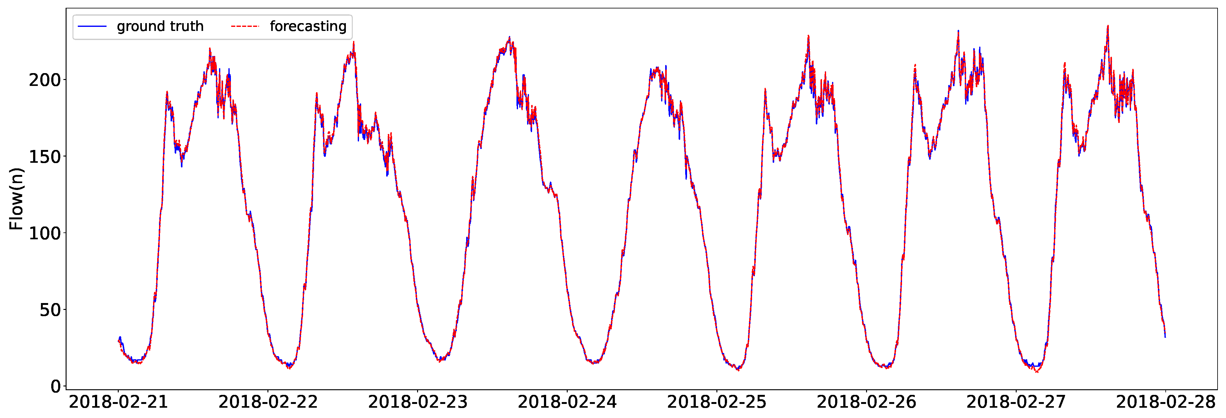
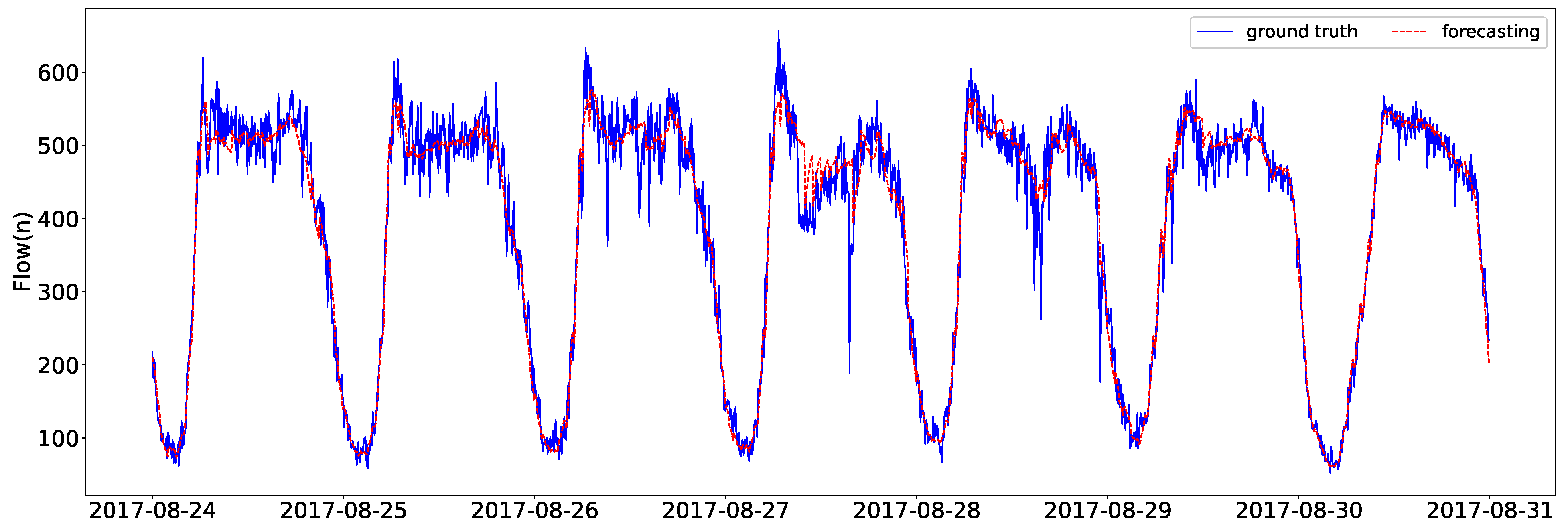
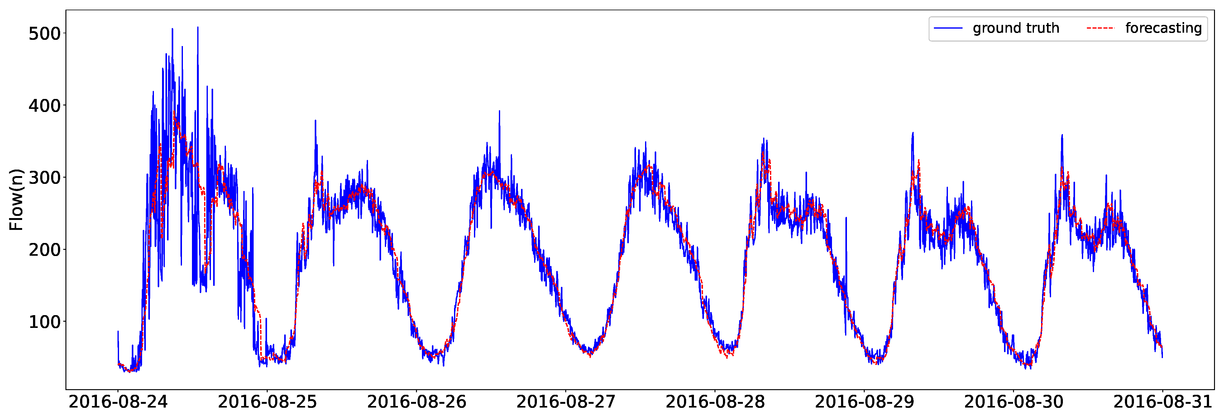
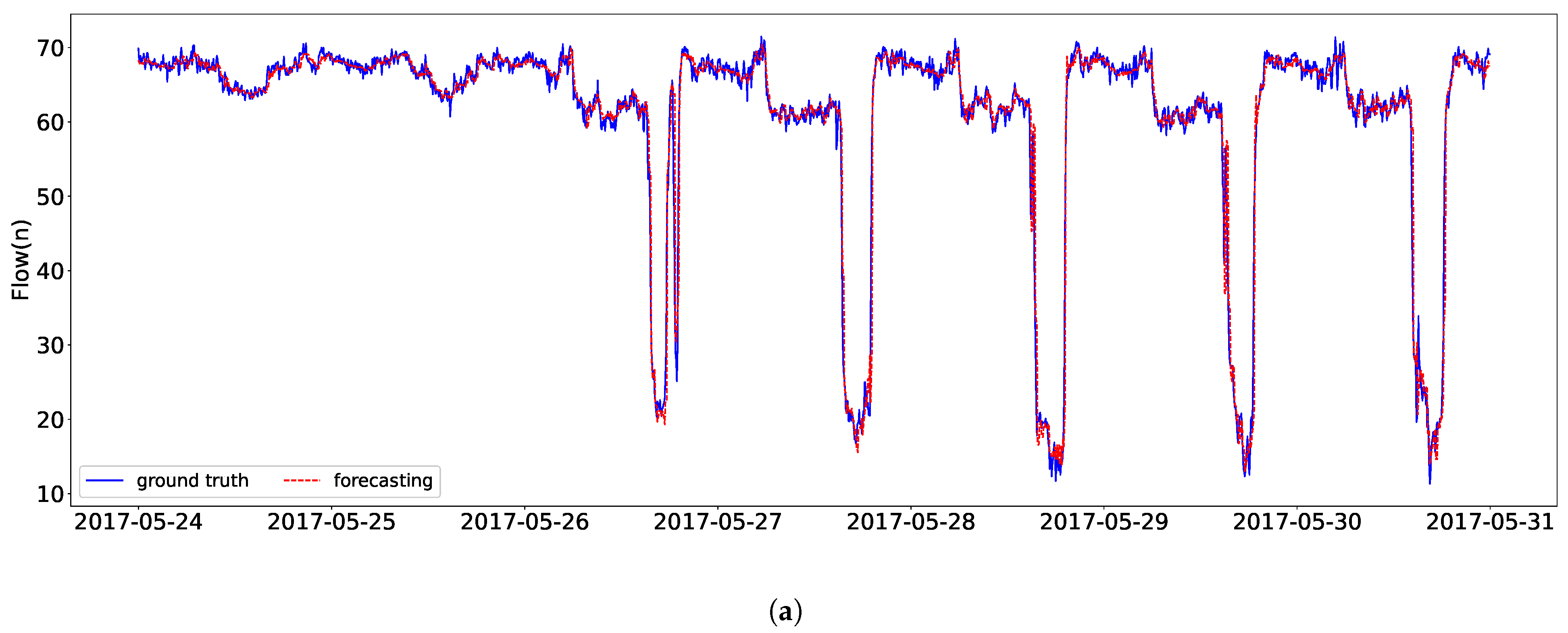
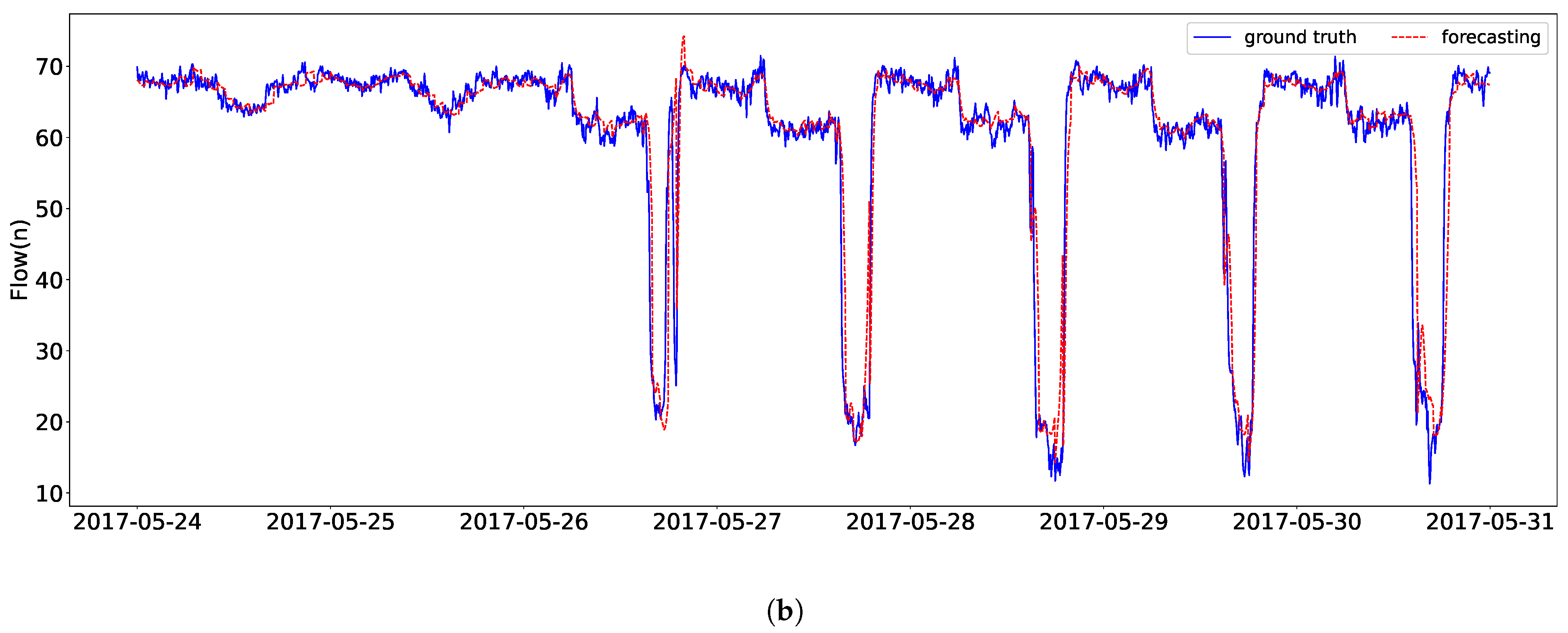
As shown in Figure 2, the forecasting curve of the STAE-BiSSSM can perfectly fit the ground truth under long-term forecasting tasks (Horizon: 12) on PeMSD4 datasets. As shown in Figure 3, Figure 4 and Figure 5, the forecasting curves of the STAE-BiSSSM can reflect the trend of the ground truth under the long-term forecasting task (Horizon: 12) well on PeMSD7, PeMSD8 and METRLA datasets with noisy data. Figure 6 shows the forecasting curves of STAE-BiSSSM under the short-term and long-term forecasting task on PeMSBAY datasets. For short-term forecasting (Horizon: 3), the forecasting curve of STAE-BiSSSM can fit the ground truth well. For long-term forecasting (Horizon: 12), the forecasting curve of STAE-BiSSSM can also reflect the trend of the ground truth well. In conclusion, STAE-BiSSSM has the ability to perform real-world traffic flow forecasting under different forecasting tasks.

3.5. Ablation Study

In order to illustrate the validity of critical components of STAE-BiSSSM, we introduce an ablation study including two variants of our model as follows:
  • FSSSM: It removes the spatio-temporal adaptive embedding E a d p and backward SSSM in STAE-BiSSSM.
  • STAE-FSSSM: It removes the backward SSSM in STAE-BiSSSM.
The results of the ablation study on PeMSD4, METRLA and PeMSBAY datasets under forecasting horizon 12 are shown in Table 6. Compared with FSSSM, MAE, RMSE and MAPE of the STAE-FSSSM decrease by 15.15%, 13.98% and 15.59% on PeMSD4 datasets; 17.35%, 16.71% and 17.76% on METRLA datasets; and 19.21%, 17.61% and 19.50% on PeMSBAY datasets, respectively. It can be seen that E a d p can enrich the representation of the feature, thus contributing the model learning. Compared with STAE-FSSSM, MAE, RMSE and MAPE of the STAE-BiSSSM decrease by 0.43%, 0.13% and 2.16% on PeMSD4 datasets; 0.62%, 0.31% and 3.36% on METRLA datasets; and 1.22%, 0.55% and 4.12% on PeMSBAY datasets. It can seen that bidirectional feature extraction of time series can be better mined to find out the dynamic change pattern of traffic flow. Therefore, each critical component of STAE-BiSSSM is necessary.

3.6. Parameter Effectiveness Analysis

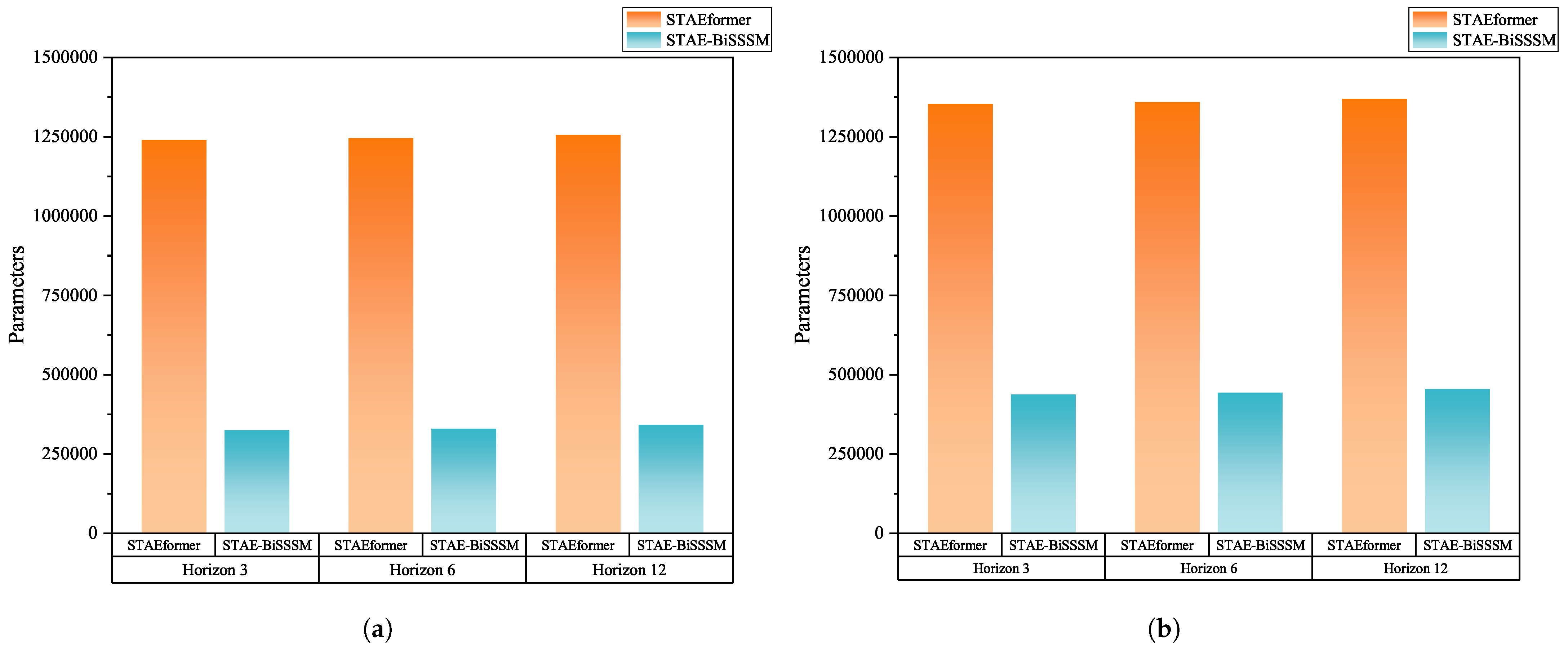
Table 7 and Figure 7 show the total trainable parameters of STAEformer and STAE-BiSSSM on METRLA and PeMSBAY datasets under different forecasting horizon. Figure 8 and Figure 9 show a comparison of three performance metrics between STAEformer and STAE-BiSSSM under different forecasting horizon. For METRLA datasets, the number of STAE-BiSSSM trainable parameters is about 26–27% of the number of STAEformer trainable parameters. For PEMSBAY datasets, the number of STAE-BiSSSM trainable parameters is about 32–33% of the number of STAEformer trainable parameters. However, the predictive performance of the STAE-BiSSSM model outperforms STAEformer on both datasets which suggests that the parameter effectiveness of STAE-BiSSSM is superior to that of STAEformer. This provides further evidence that the BiSSSM structure is more effective than the attention mechanism, and that fewer parameters can be used to retain critical information in the time series. At the same time, a smaller number of trainable parameters means that the model is cheaper to train and less demanding on hardware, which facilitates model deployment and application.

4. Conclusions

In this paper, we focus on both new structural design and the nature of the data itself. Therefore, a novel BiSSSM is proposed based on an emerging efficient model selective SSM to extract the bidirectional dependency of traffic flow time series, and spatio-temporal adaptive embedding is used for enriching the representation of features. We combine BiSSSM and STAE to obtain STAE-BiSSM, incorporating the advantages of both for better traffic flow forecasting. Comparative tests across five authoritative real-world datasets demonstrate that the STAE-BiSSSM is capable of both long- and short-term forecasting and achieves advanced performance. An ablation study illustrates that each critical component of STAE-BiSSSM is necessary. Parameter effectiveness analysis of STAE-BiSSSM suggests that STAE-BiSSSM can also achieve excellent forecasting results with a small number of parameters. In a nutshell, STAE-BiSSSM shows a promising direction for addressing the challenges in traffic forecasting. However, one a limitation is that we have not incorporated the interactions and connections between traffic flow and other traffic states into the forecasting of traffic flow. Joint traffic flow forecasting using multiple traffic features is a potential future research direction.

Author Contributions

Methodology, Duoliang Liu; software, Duoliang Liu; validation, Duoliang Liu; investigation, Xuebo Chen; resources, Qiang Qu; writing—original draft preparation, Qiang Qu; writing—review and editing, Qiang Qu and Xuebo Chen; visualization, Duoliang Liu; supervision, Xuebo Chen; funding acquisition, Xuebo Chen. All authors have read and agreed to the published version of the manuscript.

Funding

This research received no external funding.

Data Availability Statement

Acknowledgments

This research reported herein was supported by the NSFC of China under Grant No. 71571091 and 71771112.

Conflicts of Interest

The authors declare no conflicts of interest.

Abbreviations

The following abbreviations are used in this manuscript:
SSMState space models
SSSMSelective state space model
BiSSSMBidirectional selective state space model
STAESpatial–temporal adaptive embedding
STAE-BiSSSMSpatial–temporal adaptive embedding–Bidirectional selective state space model
SOTAState-of-the-art

References

  1. Chen, S.; Cheng, K.; Yang, J.; Zang, X.; Luo, Q.; Li, J. Driving Behavior Risk Measurement and Cluster Analysis Driven by Vehicle Trajectory Data. Appl. Sci. 2023, 13, 5675. [Google Scholar] [CrossRef]
  2. Huang, S.; Zhu, G.; Tang, J.; Li, W.; Fan, Z. Multi-Perspective Semantic Segmentation of Ground Penetrating Radar Images for Pavement Subsurface Objects. IEEE Trans. Intell. Transp. Syst. 2025, 26, 14339–14352. [Google Scholar] [CrossRef]
  3. Boukerche, A.; Wang, J. Machine Learning-based traffic prediction models for Intelligent Transportation Systems. Comput. Netw. 2020, 181, 107530. [Google Scholar] [CrossRef]
  4. Zhou, Z.; Yang, Z.; Zhang, Y.; Huang, Y.; Chen, H.; Yu, Z. A comprehensive study of speed prediction in transportation system: From vehicle to traffic. iScience 2022, 25, 103909. [Google Scholar] [CrossRef]
  5. Medina-Salgado, B.; Sánchez-DelaCruz, E.; Pozos-Parra, P.; Sierra, J.E. Urban traffic flow prediction techniques: A review. Sustain. Comput. Inform. Syst. 2022, 35, 100739. [Google Scholar] [CrossRef]
  6. Williams, B.M.; Hoel, L.A. Modeling and Forecasting Vehicular Traffic Flow as a Seasonal ARIMA Process: Theoretical Basis and Empirical Results. J. Transp. Eng. 2003, 129, 664–672. [Google Scholar] [CrossRef]
  7. Min, W.; Wynter, L. Real-time road traffic prediction with spatio-temporal correlations. Transp. Res. Part Emerg. Technol. 2011, 19, 606–616. [Google Scholar] [CrossRef]
  8. Hou, Q.; Leng, J.; Ma, G.; Liu, W.; Cheng, Y. An adaptive hybrid model for short-term urban traffic flow prediction. Phys. Stat. Mech. Its Appl. 2019, 527, 121065. [Google Scholar] [CrossRef]
  9. Emami, A.; Sarvi, M.; Bagloee, S.A. Short-term traffic flow prediction based on faded memory Kalman Filter fusing data from connected vehicles and Bluetooth sensors. Simul. Model. Pract. Theory 2020, 102, 102025. [Google Scholar] [CrossRef]
  10. Bakibillah, A.; Tan, Y.H.; Loo, J.Y.; Tan, C.P.; Kamal, M.; Pu, Z. Robust estimation of traffic density with missing data using an adaptive-R extended Kalman filter. Appl. Math. Comput. 2022, 421, 126915. [Google Scholar] [CrossRef]
  11. Chang, S.Y.; Wu, H.C.; Kao, Y.C. Tensor Extended Kalman Filter and its Application to Traffic Prediction. Trans. Intell. Transport. Syst. 2023, 24, 13813–13829. [Google Scholar] [CrossRef]
  12. Smola, A.J.; Schölkopf, B.S. A tutorial on support vector regression. Stat. Comput. 2004, 14, 199–222. [Google Scholar] [CrossRef]
  13. Wu, C.H.; Ho, J.M.; Lee, D. Travel-time prediction with support vector regression. IEEE Trans. Intell. Transp. Syst. 2004, 5, 276–281. [Google Scholar] [CrossRef]
  14. Yao, Z.; Shao, C.F.; Gao, Y.L. Research on methods of short-term traffic forecasting based on support vector regression. J. Beijing Jiaotong Univ. 2006, 30, 19–22. [Google Scholar]
  15. Cheng, S.; Lu, F.; Peng, P.; Wu, S. Short-term traffic forecasting: An adaptive ST-KNN model that considers spatial heterogeneity. Comput. Environ. Urban Syst. 2018, 71, 186–198. [Google Scholar] [CrossRef]
  16. Sun, Y.; Shi, Y.; Jia, K.; Zhang, Z.; Qin, L. A Dual-Stream Cross AGFormer-GPT Network for Traffic Flow Prediction Based on Large-Scale Road Sensor Data. Sensors 2024, 24, 3905. [Google Scholar] [CrossRef]
  17. Carianni, A.; Gemma, A. Overview of Traffic Flow Forecasting Techniques. IEEE Open J. Intell. Transp. Syst. 2025, 6, 848–882. [Google Scholar] [CrossRef]
  18. Chen, X.; Wu, S.; Shi, C.; Huang, Y.; Yang, Y.; Ke, R.; Zhao, J. Sensing Data Supported Traffic Flow Prediction via Denoising Schemes and ANN: A Comparison. IEEE Sens. J. 2020, 20, 14317–14328. [Google Scholar] [CrossRef]
  19. Huang, W.; Song, G.; Hong, H.; Xie, K. Deep Architecture for Traffic Flow Prediction: Deep Belief Networks With Multitask Learning. IEEE Trans. Intell. Transp. Syst. 2014, 15, 2191–2201. [Google Scholar] [CrossRef]
  20. Yasdi, R. Prediction of Road Traffic using a Neural Network Approach. Neural Comput. Appl. 1999, 8, 135–142. [Google Scholar] [CrossRef]
  21. More, R.; Mugal, A.; Rajgure, S.; Adhao, R.B.; Pachghare, V.K. Road traffic prediction and congestion control using Artificial Neural Networks. In Proceedings of the 2016 International Conference on Computing, Analytics and Security Trends (CAST), Pune, India, 19–21 December 2016; pp. 52–57. [Google Scholar] [CrossRef]
  22. Tian, Y.; Pan, L. Predicting Short-Term Traffic Flow by Long Short-Term Memory Recurrent Neural Network. In Proceedings of the 2015 IEEE International Conference on Smart City/SocialCom/SustainCom (SmartCity), Chengdu, China, 19–21 December 2015; pp. 153–158. [Google Scholar] [CrossRef]
  23. Fu, R.; Zhang, Z.; Li, L. Using LSTM and GRU neural network methods for traffic flow prediction. In Proceedings of the 2016 31st Youth Academic Annual Conference of Chinese Association of Automation (YAC), Wuhan, China, 11–13 November 2016; pp. 324–328. [Google Scholar] [CrossRef]
  24. Tian, Y.; Zhang, K.; Li, J.; Lin, X.; Yang, B. LSTM-based traffic flow prediction with missing data. Neurocomputing 2018, 318, 297–305. [Google Scholar] [CrossRef]
  25. Yang, B.; Sun, S.; Li, J.; Lin, X.; Tian, Y. Traffic flow prediction using LSTM with feature enhancement. Neurocomputing 2019, 332, 320–327. [Google Scholar] [CrossRef]
  26. Du, S.; Li, T.; Gong, X.; Yang, Y.; Horng, S.J. Traffic flow forecasting based on hybrid deep learning framework. In Proceedings of the 2017 12th International Conference on Intelligent Systems and Knowledge Engineering (ISKE), Nanjing, China, 24–26 November 2017; pp. 1–6. [Google Scholar] [CrossRef]
  27. Liu, Y.; Zheng, H.; Feng, X.; Chen, Z. Short-term traffic flow prediction with Conv-LSTM. In Proceedings of the 2017 9th International Conference on Wireless Communications and Signal Processing (WCSP), Nanjing, China, 11–13 October 2017; pp. 1–6. [Google Scholar] [CrossRef]
  28. Duan, Z.; Yang, Y.; Zhang, K.; Ni, Y.; Bajgain, S. Improved Deep Hybrid Networks for Urban Traffic Flow Prediction Using Trajectory Data. IEEE Access 2018, 6, 31820–31827. [Google Scholar] [CrossRef]
  29. Ma, D.; Sheng, B.; Jin, S.; Ma, X.; Gao, P. Short-Term Traffic Flow Forecasting by Selecting Appropriate Predictions Based on Pattern Matching. IEEE Access 2018, 6, 75629–75638. [Google Scholar] [CrossRef]
  30. Yao, H.; Tang, X.; Wei, H.; Zheng, G.; Li, Z. Revisiting Spatial-Temporal Similarity: A Deep Learning Framework for Traffic Prediction. arXiv 2018, arXiv:1803.01254. [Google Scholar] [CrossRef]
  31. Narmadha, S.; Vijayakumar, V. Spatio-Temporal vehicle traffic flow prediction using multivariate CNN and LSTM model. Mater. Today Proc. 2023, 81, 826–833. [Google Scholar] [CrossRef]
  32. Zhang, X.; Huang, K.; Liu, C.; Xu, X. Urban Short - Term Traffic Flow Prediction Algorithm Based on CNN-LSTM Model. In Proceedings of the 2023 3rd International Conference on Consumer Electronics and Computer Engineering (ICCECE), Guangzhou, China, 6–8 January 2023; pp. 214–217. [Google Scholar] [CrossRef]
  33. Zhao, Z.; Chen, W.; Wu, X.; Chen, P.C.Y.; Liu, J. LSTM network: A deep learning approach for short-term traffic forecast. IET Intell. Transp. Syst. 2017, 11, 68–75. [Google Scholar] [CrossRef]
  34. Yu, B.; Yin, H.; Zhu, Z. Spatio-Temporal Graph Convolutional Networks: A Deep Learning Framework for Traffic Forecasting. In Proceedings of the Twenty-Seventh International Joint Conference on Artificial Intelligence. International Joint Conferences on Artificial Intelligence Organization, Stockholm, Sweden, 13–19 July 2018; pp. 3634–3640. [Google Scholar] [CrossRef]
  35. Cao, D.; Wang, Y.; Duan, J.; Zhang, C.; Zhu, X.; Huang, C.; Tong, Y.; Xu, B.; Bai, J.; Tong, J.; et al. Spectral Temporal Graph Neural Network for Multivariate Time-series Forecasting. arXiv 2021, arXiv:2103.07719. [Google Scholar] [CrossRef]
  36. Chen, Y.; Segovia-Dominguez, I.; Gel, Y.R. Z-GCNETs: Time Zigzags at Graph Convolutional Networks for Time Series Forecasting. arXiv 2021, arXiv:2105.04100. [Google Scholar] [CrossRef]
  37. Diao, Z.; Wang, X.; Zhang, D.; Liu, Y.; Xie, K.; He, S. Dynamic spatial-temporal graph convolutional neural networks for traffic forecasting. In Proceedings of the Thirty-Third AAAI Conference on Artificial Intelligence and Thirty-First Innovative Applications of Artificial Intelligence Conference and Ninth AAAI Symposium on Educational Advances in Artificial Intelligence, Honolulu, HI, USA, 27 January–1 February 2019. [Google Scholar] [CrossRef]
  38. Fang, Z.; Long, Q.; Song, G.; Xie, K. Spatial-Temporal Graph ODE Networks for Traffic Flow Forecasting. In Proceedings of the 27th ACM SIGKDD Conference on Knowledge Discovery & Data Mining, New York, NY, USA, 14–18 August 2021; pp. 364–373. [Google Scholar] [CrossRef]
  39. Guo, K.; Hu, Y.; Sun, Y.; Qian, S.; Gao, J.; Yin, B. Hierarchical Graph Convolution Network for Traffic Forecasting. Proc. AAAI Conf. Artif. Intell. 2021, 35, 151–159. [Google Scholar] [CrossRef]
  40. Li, Y.; Yu, R.; Shahabi, C.; Liu, Y. Diffusion Convolutional Recurrent Neural Network: Data-Driven Traffic Forecasting. arXiv 2018, arXiv:1707.01926. [Google Scholar] [CrossRef]
  41. Zhao, L.; Song, Y.; Zhang, C.; Liu, Y.; Wang, P.; Lin, T.; Deng, M.; Li, H. T-GCN: A Temporal Graph Convolutional Network for Traffic Prediction. IEEE Trans. Intell. Transp. Syst. 2020, 21, 3848–3858. [Google Scholar] [CrossRef]
  42. Bai, L.; Yao, L.; Li, C.; Wang, X.; Wang, C. Adaptive Graph Convolutional Recurrent Network for Traffic Forecasting. arXiv 2020, arXiv:2007.02842. [Google Scholar] [CrossRef]
  43. Wu, Z.; Pan, S.; Long, G.; Jiang, J.; Zhang, C. Graph WaveNet for Deep Spatial-Temporal Graph Modeling. arXiv 2019, arXiv:1906.00121. [Google Scholar]
  44. Shang, C.; Chen, J.; Bi, J. Discrete Graph Structure Learning for Forecasting Multiple Time Series. arXiv 2021, arXiv:2101.06861. [Google Scholar] [CrossRef]
  45. Wu, Z.; Pan, S.; Long, G.; Jiang, J.; Chang, X.; Zhang, C. Connecting the Dots: Multivariate Time Series Forecasting with Graph Neural Networks. arXiv 2020, arXiv:2005.11650. [Google Scholar] [CrossRef]
  46. Jiang, R.; Wang, Z.; Yong, J.; Jeph, P.; Chen, Q.; Kobayashi, Y.; Song, X.; Fukushima, S.; Suzumura, T. Spatio-Temporal Meta-Graph Learning for Traffic Forecasting. arXiv 2023, arXiv:2211.14701. [Google Scholar] [CrossRef]
  47. Zhang, Q.; Chang, J.; Meng, G.; Xiang, S.; Pan, C. Spatio-Temporal Graph Structure Learning for Traffic Forecasting. Proc. AAAI Conf. Artif. Intell. 2020, 34, 1177–1185. [Google Scholar] [CrossRef]
  48. Zheng, C.; Fan, X.; Wang, C.; Qi, J. GMAN: A Graph Multi-Attention Network for Traffic Prediction. arXiv 2019, arXiv:1911.08415. [Google Scholar] [CrossRef]
  49. Jiang, J.; Han, C.; Zhao, W.X.; Wang, J. PDFormer: Propagation Delay-Aware Dynamic Long-Range Transformer for Traffic Flow Prediction. Proc. AAAI Conf. Artif. Intell. 2023, 37, 4365–4373. [Google Scholar] [CrossRef]
  50. Wu, H.; Xu, J.; Wang, J.; Long, M. Autoformer: Decomposition Transformers with Auto-Correlation for Long-Term Series Forecasting. arXiv 2022, arXiv:2106.13008. [Google Scholar]
  51. Zhou, G.; Guo, X.; Liu, Z.; Li, T.; Li, Q.; Xu, K. TrafficFormer: An Efficient Pre-trained Model for Traffic Data. In Proceedings of the 2025 IEEE Symposium on Security and Privacy (SP), San Francisco, CA, USA, 12–15 May 2025; pp. 1844–1860. [Google Scholar] [CrossRef]
  52. Pu, B.; Liu, J.; Kang, Y.; Chen, J.; Yu, P.S. MVSTT: A Multiview Spatial-Temporal Transformer Network for Traffic-Flow Forecasting. IEEE Trans. Cybern. 2024, 54, 1582–1595. [Google Scholar] [CrossRef]
  53. Shao, Z.; Zhang, Z.; Wang, F.; Wei, W.; Xu, Y. Spatial-Temporal Identity: A Simple yet Effective Baseline for Multivariate Time Series Forecasting. arXiv 2022, arXiv:2208.05233. [Google Scholar] [CrossRef]
  54. Liu, H.; Dong, Z.; Jiang, R.; Deng, J.; Deng, J.; Chen, Q.; Song, X. Spatio-Temporal Adaptive Embedding Makes Vanilla Transformer SOTA for Traffic Forecasting. In Proceedings of the 32nd ACM International Conference on Information and Knowledge Management, New York, NY, USA, 21–25 October 2023; pp. 4125–4129. [Google Scholar] [CrossRef]
  55. Sun, Y.; Dong, L.; Huang, S.; Ma, S.; Xia, Y.; Xue, J.; Wang, J.; Wei, F. Retentive Network: A Successor to Transformer for Large Language Models. arXiv 2023, arXiv:2307.08621. [Google Scholar] [CrossRef]
  56. Peng, B.; Alcaide, E.; Anthony, Q.; Albalak, A.; Arcadinho, S.; Biderman, S.; Cao, H.; Cheng, X.; Chung, M.; Grella, M.; et al. RWKV: Reinventing RNNs for the Transformer Era. arXiv 2023, arXiv:2305.13048. [Google Scholar] [CrossRef]
  57. Gu, A.; Dao, T. Mamba: Linear-Time Sequence Modeling with Selective State Spaces. arXiv 2024, arXiv:2312.00752. [Google Scholar]
  58. Gu, A.; Goel, K.; Ré, C. Efficiently Modeling Long Sequences with Structured State Spaces. arXiv 2022, arXiv:2111.00396. [Google Scholar] [CrossRef]
  59. Zhang, B.; Sennrich, R. Root Mean Square Layer Normalization. arXiv 2019, arXiv:1910.07467. [Google Scholar] [CrossRef]
  60. Cui, Y.; Xie, J.; Zheng, K. Historical Inertia: An Ignored but Powerful Baseline for Long Sequence Time-series Forecasting. CoRR 2021, arXiv:2103.16349. [Google Scholar]
  61. Deng, J.; Chen, X.; Jiang, R.; Song, X.; Tsang, I.W. ST-Norm: Spatial and Temporal Normalization for Multi-variate Time Series Forecasting. In Proceedings of the 27th ACM SIGKDD Conference on Knowledge Discovery & Data Mining, New York, NY, USA, 14–18 August 2021; pp. 269–278. [Google Scholar] [CrossRef]
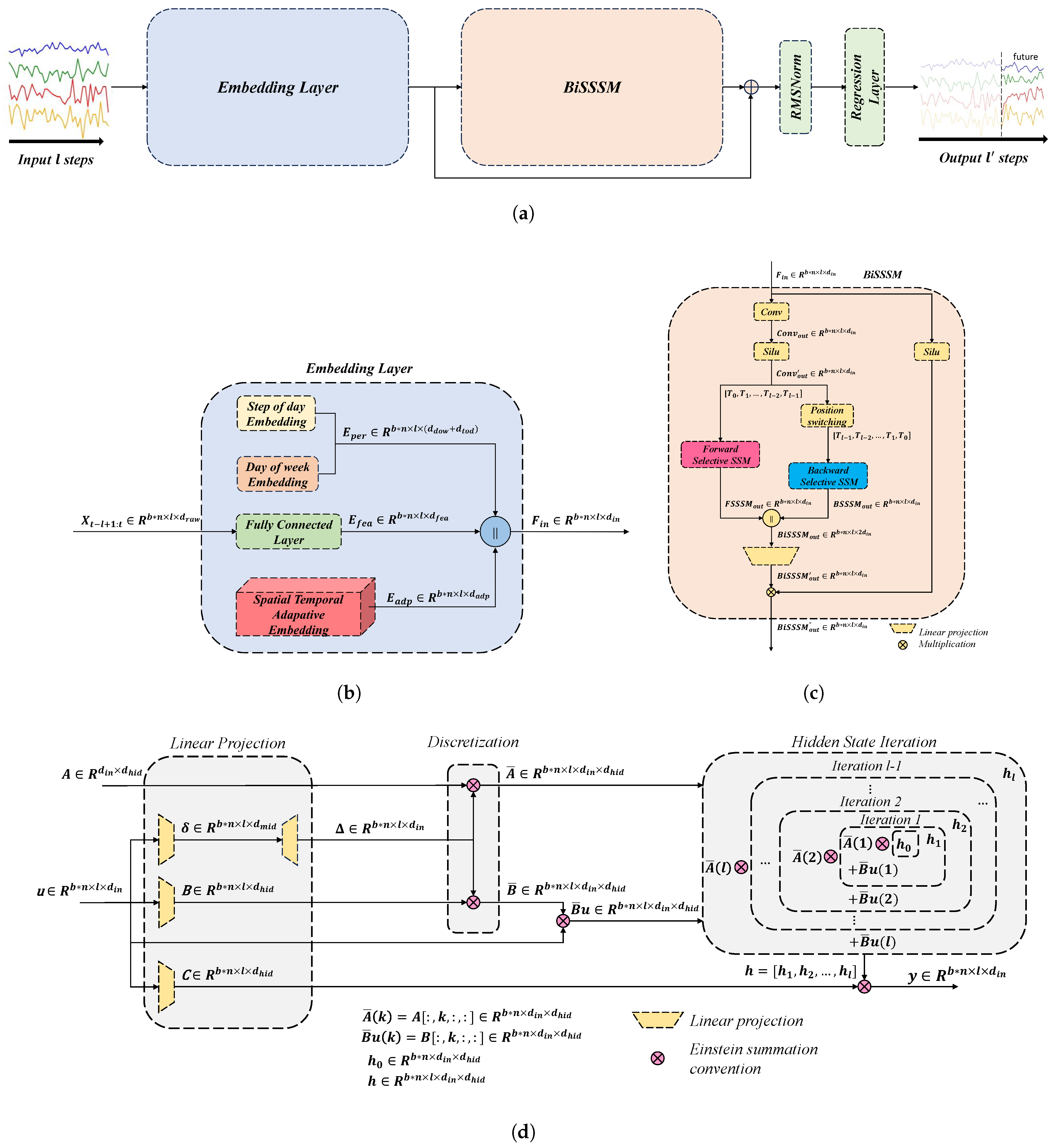
Figure 1. (a) An overall structure of STAE-BiSSSM. (b) Structure of embedding layer. (c) Structure of BiSSSM. (d) Structure of SSSM.
Ijgi 14 00388 g001
Figure 2. Actual forecasting of the STAE-BiSSSM model on the PeMSD4 datasets for the road where sensor No. 200 is located from 2018-2-21 to 2018-2-28.
Ijgi 14 00388 g002
Figure 3. Actual forecasting of the STAE-BiSSSM model on the PeMSD7 datasets for the road where sensor No. 800 is located from 2017-8-24 to 2017-8-31.
Ijgi 14 00388 g003
Figure 4. Actual forecasting of the STAE-BiSSSM model on the PeMSD8 datasets for the road where sensor No. 150 is located from 2016-8-24 to 2016-8-31.
Ijgi 14 00388 g004
Figure 5. Actual forecasting of the STAE-BiSSSM model on the METRLA datasets for the road where sensor No. 200 is located from 2012-6-23 to 2012-6-30.
Ijgi 14 00388 g005
Figure 6. Actual forecasting of the STAE-BiSSSM model on the PeMSBAY datasets for the road where sensor No. 200 is located from 2017-5-24 to 2017-5-31. (a) Forecasting curves under forecasting horizon 15 min. (b) Forecasting curves under forecasting horizon 60 min.
Ijgi 14 00388 g006aIjgi 14 00388 g006b
Figure 7. (a) Total trainable parameters of STAEformer and STAE-iSSSM on METRLA datasets under different forecasting horizons. (b) Total trainable parameters of STAEformer and STAE-iSSSM on PeMSBAY datasets under different forecasting horizons.
Ijgi 14 00388 g007
Figure 8. (a) MAE of STAEformer and STAE-BiSSSM on METRLA datasets with different forecasting horizons. (b) RMSE of STAEformer and STAE-BiSSSM on METRLA datasets with different forecasting horizons. (c) MAPE of STAEformer and STAE-BiSSSM on METRLA datasets with different forecasting horizons.
Ijgi 14 00388 g008
Figure 9. (a) MAE of STAEformer and STAE-BiSSSM on PeMSBAY datasets with different forecasting horizons. (b) RMSE of STAEformer and STAE-BiSSSM on PeMSBAY datasets with different forecasting horizons. (c) MAPE of STAEformer and STAE-BiSSSM on PeMSBAY datasets with different forecasting horizons.
Ijgi 14 00388 g009
Table 1. Details of traffic flow datasets in experiments.
DatasetNumber of SensorsTime StepsSample IntervalTime RangeLocation
PeMSD430716,9925 min01/2018–02/2018California District 4
PeMSD788328,2245 min05/2017–08/2017California District 7
PeMSD817017,8565 min07/2016–08/2016California District 8
METRLA20734,2725 min03/2012–06/2012Los Angeles
PeMSBAY32552,1165 min01/2017–05/2017San Francisco Bay Area
Table 2. Description and details of model parameters.
HyperparameterDescriptionDimension Size
d f e a Embedding dimension of feature embedding24
d t o d Embedding dimension of time of day embedding24
d d o w Embedding dimension of day-of-week embedding24
d a d p Embedding dimension of spatial–temporal adaptive embedding80
d c o n v Size of convolution kernel5
d h i d Dimension of hidden state64
d m i d Dimension of middle-rank state16
Table 3. Predictive metrics of STAE-BiSSSM and other baseline models on PeMSD4, PeMSD7 and PeMSD8 datasets.
DatasetPeMSD4PeMSD7PeMSD8
MetricMAERMSEMAPEMAERMSEMAPEMAERMSEMAPE
Model
HI42.3561.6629.92%49.0371.1822.75%36.6650.4521.63%
GWNet18.5329.9212.89%20.4733.478.61%14.4023.399.21%
DCRNN19.6331.2613.59%21.1634.149.02%15.2224.1710.21%
AGCRN19.3831.2513.40%20.5734.408.74%15.3224.4110.03%
STGCN19.5731.3813.44%21.7435.279.24%16.0825.3910.60%
GTS20.9632.9514.66%22.1535.109.38%16.4926.0810.54%
MTGNN19.1731.7013.37%20.8934.069.00%15.1824.2410.20%
STNorm18.9630.9812.69%20.5034.668.75%15.4124.779.76%
GMAN19.1431.6013.19%20.9734.109.05%15.3124.9210.13%
STAE-BiSSSM
(Ours)
18.4630.1612.24%19.9133.168.43%13.8423.239.24%
Table 4. Predictive metrics of STAE-BiSSSM and other baseline models on METRLA.
DatasetMETRLA
Horizon15 min30 min60 min
Metric  MAE  RMSE  MAPE  MAE  RMSE  MAPE  MAE  RMSE  MAPE
Model
HI6.8014.2116.72%6.8014.2116.72%6.8014.2010.15%
GWNet2.695.156.99%3.086.208.47%3.517.289.96%
DCRNN2.675.166.86%3.126.278.42%3.547.4710.32%
AGCRN2.855.537.63%3.206.529.00%3.597.4510.47%
STGCN2.755.297.10%3.156.358.62%3.607.4310.35%
GTS2.755.277.12%3.146.338.62%3.597.4410.25%
MTGNN2.695.166.89%3.056.138.16%3.477.219.70%
STNorm2.815.577.40%3.186.598.47%3.577.5110.24%
GMAN2.805.557.41%3.126.498.73%3.447.3510.07%
PDFormer2.835.457.77%3.206.469.19%3.627.4710.91%
STID2.825.537.75%3.196.579.39%3.557.5510.95%
STAEformer2.655.116.85%2.976.008.13%3.347.029.70%
STAE-BiSSSM
(Ours)
2.604.926.75%2.865.597.88%3.226.519.49%
Table 5. Predictive metrics of STAE-BiSSSM and other baseline models on PeMSBAY.
DatasetPeMSBAY
Horizon15 min30 min60 min
MetricMAERMSEMAPEMAERMSEMAPEMAERMSEMAPE
Model
HI3.067.056.85%3.067.046.84%3.057.036.83%
GWNet1.302.732.71%1.633.733.73%1.994.604.71%
DCRNN1.312.762.73%1.653.753.71%1.974.604.68%
AGCRN1.352.882.91%1.673.823.81%1.944.504.55%
STGCN1.362.882.86%1.703.843.79%2.024.634.72%
GTS1.372.922.85%1.723.863.88%2.064.604.88%
MTGNN1.332.802.81%1.663.773.75%1.954.504.62%
STNorm1.332.822.76%1.653.773.66%1.924.454.46%
GMAN1.352.902.87%1.653.823.74%1.924.494.52%
PDFormer1.322.832.78%1.643.793.71%1.914.434.51%
STID1.312.792.78%1.643.733.73%1.914.424.55%
STAEformer1.312.782.76%1.623.683.62%1.884.344.41%
STAE-BiSSSM
(Ours)
1.132.332.28%1.362.962.93%1.623.633.72%
Table 6. Ablation study on PeMSD4, METRLA and PeMSBAY datasets.
Dataset ModelFSSSMSTAE-FSSSMSTAE-BiSSSM
Metric
PeMSD4MAE21.8518.5418.46
RMSE35.1130.2030.16
MAPE14.82%12.51%12.24%
METRLAMAE3.923.243.22
RMSE7.846.536.51
MAPE11.94%9.82%9.49%
PeMSBAYMAE2.031.641.62
RMSE4.433.653.63
MAPE4.82%3.88%3.72%
Table 7. Total trainable parameters of STAEformer and STAE-BiSSSM on METRLA and PEMSBAY datasets under different forecasting horizon.
DatasetsModelsSTAEformerSTAE-BiSSSM
Horizon
METRLA3 (15 min)1,242,555327,195
6 (30 min)1,248,030332,670
9 (60 min)1,258,980343,620
PeMSBAY3 (15 min)1,355,835440,475
6 (30 min)1,361,310445,950
9 (60 min)1,372,260456,900
Disclaimer/Publisher’s Note: The statements, opinions and data contained in all publications are solely those of the individual author(s) and contributor(s) and not of MDPI and/or the editor(s). MDPI and/or the editor(s) disclaim responsibility for any injury to people or property resulting from any ideas, methods, instructions or products referred to in the content.