Article

Assessing Spatial Accessibility Uncertainty with Dempster–Shafer Theory: A Comparison of Potential and Revealed Accessibility

by
Roya Esmaeili Tajabadi
1,
Parham Pahlavani
1,
Amin Hosseinpoor Milaghardan
2 and
Christophe Claramunt
3,*
1
Center of Excellence in Geomatics Engineering in Disaster Management, School of Surveying and Geospatial Engineering, College of Engineering, University of Tehran, Tehran 1417614411, Iran
2
Department of Geographic Information Systems, Faculty of Civil and Surveying Engineering, Graduate University of Advanced Technology, Kerman 7631885356, Iran
3
Naval Academy Research Institute, 29160 Lanvéoc, France
*
Author to whom correspondence should be addressed.
ISPRS Int. J. Geo-Inf. 2025, 14(10), 370; https://doi.org/10.3390/ijgi14100370
Submission received: 8 July 2025 / Revised: 3 September 2025 / Accepted: 12 September 2025 / Published: 23 September 2025

Abstract

This study introduces a framework for comparing and integrating revealed and potential accessibility maps, using the Dempster–Shafer theory to identify regions with varying spatial accessibility while accounting for uncertainty. It presents a method for determining revealed accessibility from individuals’ trajectory data, weighting accessibility inversely to the square of uncertainty. This dual approach aids urban planners in making more reliable decisions. The methodology is applied to supply centers, including shops, restaurants, and sports centers, using data from the Mobile Data Challenge (MDC) in Vaud, Switzerland. The results show good access to shops in the northwestern and southeastern regions and good access to restaurants in the eastern regions. The final maps indicate that areas with low access to sports centers form the highest proportion (62.7%) of regions with low access, while those with low access to shopping centers form the lowest (9.3%). The findings suggest the need for more sports centers in Nyon and Jura-Nord Vaudois and more accessible restaurants in Nyon and southern Aigle. Additionally, the analysis reveals that lower station densities correlate with smaller discrepancies between real and expected accessibilities, while higher population densities are linked to lower uncertainty, underscoring the importance of considering density in spatial accessibility assessments.

1. Introduction

Over the past few decades, rapid urbanization has led to significant population growth in cities, with projections indicating that nearly 66% of the global population will reside in urban areas by 2050 [1]. Urban areas provide a variety of opportunities, services, and facilities, such as employment, healthcare access, and sociocultural participation, which are essential for improving residents’ quality of life [2]. However, inadequate spatial distribution of facilities and poor accessibility can create inequalities, leaving certain neighborhoods underserved and negatively impacting residents’ quality of life [3]. In this study, “high accessibility” refers to areas where individuals have greater access to services and opportunities, while “low accessibility” denotes regions with limited access due to barriers such as distance, cost, or inadequate infrastructure. Understanding how urban facilities are distributed and accessed is critical for promoting equitable development, achieving uniform service delivery, and ensuring easy access for all residents [4,5].
Spatial accessibility has been widely studied in various fields, such as urban and transport planning, housing development, and quality-of-life assessments [6,7]. Previous studies primarily focused on potential accessibility (PA), the theoretical access to facilities such as health centers [8,9], recreational areas [10], food stores [11,12], and green spaces [13], using methods ranging from cumulative measures to advanced, gravity-based approaches [14]. While these evaluations provide insights into urban planning, they often overlook whether individuals actually use facilities as predicted by potential accessibility maps.
The discrepancy between potential accessibility and revealed accessibility (RA), which reflects real-world usage patterns derived from individuals’ movement data, remains underexplored [15]. Such discrepancies can arise from factors like personal preferences, cultural norms, service quality, security concerns, or operating hours of facilities, which may prompt individuals to travel further for better services [16,17]. Therefore, this study adopts the premise that integrating RA and PA can provide a more comprehensive understanding of accessibility patterns, bridging the gap between theoretical models and real-world behavior. While not having been tested as a formal hypothesis, this premise serves as the foundation for the conceptual and empirical work presented here. Accordingly, the central research question of this study is whether there are significant differences between potential and revealed accessibility across urban regions. A further focus is on identifying the empirical advantages provided by the Dempster–Shafer theory (DST) in integrating the two. In addressing this, attention is also given to two dimensions of uncertainty: subjective uncertainty, which arises from individual behavioral biases and preferences; structural uncertainty, which results from data limitations and modeling assumptions. Classical spatial–behavioral theories such as time geography and activity-based modeling have traditionally studied individuals’ space–time constraints and activity choices. However, these approaches are limited in explicitly handling uncertainty and reconciling conflicting evidence from heterogeneous data sources. DST complements them by offering a probabilistic–evidential framework that quantifies uncertainty and integrates multiple, potentially conflicting sources of evidence. While DST does not model individual decision-making processes in as much behavioral detail as activity-based approaches, it provides a systematic way to incorporate uncertainty into accessibility assessments.
Moreover, uncertainty in determining spatial accessibility remains a persistent challenge that has received limited attention [18,19]. Traditional spatial models often rely on fixed travel times and static conditions, which oversimplify real-world complexities such as traffic congestion, demand fluctuations, and network disruptions [20]. Addressing uncertainty enables a more robust evaluation of accessibility by accounting for variability and incomplete information, thereby improving decision making for urban planners.
This study specifically addresses spatial uncertainty, arising from incomplete and conflicting spatial data, by employing Dempster–Shafer theory (DST). DST evaluates uncertainty systematically through three components: belief, disbelief, and uncertainty. This makes it particularly suitable for handling complex spatial dynamics. The choice of DST is motivated by its ability to handle conflicting evidence and manage situations where data are incomplete or imprecise, which is common in urban studies. In our context, DST provides a reliable method for integrating spatial data with varying degrees of certainty, facilitating more accurate assessments of accessibility in urban areas. However, it is important to note that our study does not explicitly model dynamic factors such as travel time variability, demand fluctuations, or network disruptions. Instead, the focus is on handling spatial uncertainties to ensure more equitable and reliable accessibility assessments.
In summary, this research aims to bridge the existing gaps, as follows:
  • By addressing the uncertainty in identifying regions with high and low accessibility;
  • By developing a method to calculate revealed accessibility using individuals’ trajectory data;
  • By proposing a framework to compare and integrate potential accessibility with revealed accessibility for supply centers.
The rest of this paper is organized as follows: Section 2 discusses the research background, Section 3 explains the methodology, Section 4 describes the data and study area, Section 5 presents the results and discussion, and Section 6 concludes with key findings and implications.

2. Research Basics and Background

2.1. Defining and Measuring Spatial Accessibility

Accessibility is defined in various ways across studies: “the potential of opportunities for interaction” [21]; “the ease with which any land use activity can be reached from a location using a particular transport system” [22]. Broadly, it refers to the ease of reaching desired infrastructure and services from a geographic area [5,9,14]. Geurs and Van Wee (2004) identify four components of accessibility: land use, transport, temporal, and individual. Land use reflects the quality and quantity of supplies and their demand, while transport describes the availability of transport infrastructures [6]. Temporal components account for service hours and individuals’ time constraints, and individual components reflect sociodemographic characteristics. While accessibility focuses on reaching specific services or opportunities, it differs from activity spaces, which represent the spatial extent of locations individuals visit during their routines [23]. This distinction ensures accessibility measures remain focused on analyzing access to specific services without conflating broader mobility patterns.
Accessibility can be assessed through four main approaches, each tailored to different dimensions of analysis [6]:
  • Infrastructure-based measures evaluate transport system performance, such as travel speeds or congestion levels, providing insights into system efficiency.
  • Location-based measures focus on spatial distribution, using cumulative opportunity or gravity models to capture access dynamics. Cumulative models count the number of opportunities within a defined threshold, while gravity models dynamically weight opportunities based on travel impedance, offering a more nuanced depiction of spatial interactions [5,24].
  • Person-based measures examine accessibility through individual constraints, such as time budgets and activity schedules. This approach offers a more granular perspective by capturing how temporal and spatial constraints shape accessibility [25].
  • Utility-based measures incorporate user preferences and economic principles like consumer surplus, linking accessibility to user satisfaction and choice behavior. These measures emphasize the economic and subjective dimensions of accessibility, enabling a better understanding of how individuals perceive and benefit from available services [26].
In urban planning and geographical studies, the focus often centers on methods that integrate land use and transportation components due to their critical role in shaping accessibility [6]. These methods typically consider three key parameters: the location of suppliers (infrastructure and services), the location of demand (population centers), and the mobility factors (travel costs or time) between them [5]. Most spatial accessibility assessment methods are founded on distance or travel time to distribution centers, all of which assume that individuals are potential users of these services [8,9].
Several methods are used to quantify accessibility, each with distinct advantages and limitations:
  • Distance to the nearest supply center: This straightforward approach calculates accessibility based on proximity, using metrics like Euclidean or road network-based travel time distances [9].
  • Number of supply centers within a specified travel time: This method accounts for the density of service provision within a reachable distance, reflecting urban accessibility dynamics [8].
  • Supply–demand balance: This ratio-based method evaluates the distribution balance between supply and demand centers within defined geographic areas [27]. However, it may oversimplify the interaction dynamics between different centers.
  • Cumulative Opportunity Models: These models assess accessibility by counting the number of opportunities (e.g., jobs or services) within a specified distance or travel time. They are effective for identifying local disparities, and particularly useful in urban areas [28]. However, they do not account for opportunity attractiveness (e.g., size or capacity) or the declining influence of distance beyond the threshold. Despite these limitations, they remain a practical tool for local analyses [8].
  • Gravity models: Gravity models dynamically measure accessibility by weighting opportunities based on their attractiveness (e.g., size or capacity) and the cost of travel, such as distance or time. They include decay functions, like exponential or power decay, to reflect the decreasing influence of accessibility as distance increases [5,8]. Unlike cumulative models, gravity models capture broader spatial interactions, enabling detailed regional or national analyses. Enhanced versions, such as those accounting for competition among demand locations and prioritizing closer supply centers, provide a comprehensive view of accessibility by linking proximity with population size [14,24].
The Two-Step Floating Catchment Area (2SFCA) model, derived from gravity-based principles, simplifies accessibility analysis by using fixed access radii or thresholds instead of continuous distance functions, which enhances implementation and interpretability [29,30]. However, its assumption of uniform accessibility within the radius and exclusion of outlying areas limits its real-world applicability. To address these issues, the Enhanced 2SFCA (E2SFCA) model introduces variable access radii and Gaussian weighting functions, refining accessibility analysis by capturing spatial variability and service availability more effectively [31].
A complementary method for categorizing accessibility measures is presented by Wu and Levinson (2020), who propose a unified framework systematically grouping these measures into two primary approaches: Primal and Dual [28]. Primal measures focus on the quantity of opportunities reachable within a given cost threshold, offering localized insights into accessibility disparities. Dual measures, in contrast, evaluate the travel cost required to access a specified number of opportunities, providing a broader, system-wide perspective. This framework bridges the conceptual divide between cumulative opportunity and gravity models by emphasizing their shared foundational components: travel costs and reachable opportunities. By introducing this systematic distinction, the framework clarifies how various assumptions regarding travel impedance and opportunity distribution influence accessibility outcomes. This enhances the adaptability and theoretical coherence of accessibility measures, enabling their application across diverse contexts and facilitating more precise, context-sensitive evaluations.
Building on these advancements, the E2SFCA model was adopted in this study for its ability to address spatial variability through flexible catchment radii and Gaussian weighting functions, offering a balance between precision and practicality. While E2SFCA refines traditional gravity-based methods, it still faces limitations in capturing demand-side dynamics such as user preferences, resource competition, and socioeconomic constraints. For the objectives of this study, examining spatial patterns of access, E2SFCA offers a robust balance between simplicity and precision, effectively integrating both supply-side and demand-side considerations. These features make it particularly suited to urban accessibility analyses, capturing the heterogeneous distribution of services and population demand while refining traditional gravity-based methods.

2.2. Potential Versus Revealed Accessibility

Accessibility is commonly distinguished into two dimensions: potential (normative or prescriptive) and revealed (positive or descriptive) [32,33,34]. Potential accessibility reflects the theoretical opportunities available to individuals in an idealized environment, assuming minimal barriers. It expands the “choice set” available to residents, offering divere opportunities that enhance flexibility and quality of life, even if they are not fully utilized. In contrast, revealed accessibility reflects actual service usage derived from observed behaviors and choices, highlighting the practical realities and barriers individuals face. These barriers can be spatial (e.g., availability and proximity) or non-spatial (e.g., affordability, cultural acceptability, and accommodation) [8]. While potential accessibility identifies opportunities and expands the range of choices available, revealed accessibility highlights discrepancies and limitations in service utilization. For instance, a region with high potential accessibility to healthcare services may exhibit low revealed accessibility due to affordability issues or a lack of trust in service providers. Integrating these dimensions helps identify such barriers, offering a comprehensive framework for addressing spatial disparities and informing equitable urban planning strategies.
Comparative studies further illustrate the importance of integrating these dimensions. For example, Lin et al. (2005) observed that individuals traveled nearly twice the distance to pharmacies compared to what potential accessibility models predicted [16]. Similarly, Casas et al. (2017) found that actual hospital travel times were approximately six times longer than estimates derived from potential models [34]. These findings emphasize the need to complement potential models with real-world data to better understand accessibility patterns and address inequities effectively.
To further clarify the concept of revealed accessibility, it is important to differentiate it from broader mobility patterns captured by “activity spaces”. Activity spaces, as defined by Patterson and Farber (2015), encompass the spatial extent of locations individuals visit during their daily routines, reflecting general mobility and potential travel paths [23]. In contrast, revealed accessibility focuses specifically on actual service use and the barriers restricting access to essential services. This distinction allows for a more targeted understanding of service gaps, enabling the identification of actionable solutions within the broader framework of accessibility analysis.
In addition to potential and revealed accessibility, perceived accessibility is another critical dimension that enriches our understanding of accessibility dynamics. Perceived accessibility focuses on individuals’ subjective evaluations of how easily they can access and utilize services, reflecting experiential and psychological aspects such as feelings of safety, trust in providers, and service quality [17,35]. Unlike potential and revealed accessibility, which are often quantified using spatial and behavioral data, perceived accessibility requires specialized information collected through questionnaires, such as the perceived accessibility scale (PAC), first introduced by Lättman et al. (2016) [36] and further developed by the same authors in 2018 [35]. While this study primarily addresses potential and revealed accessibility, acknowledging the role of perceived accessibility highlights its importance, particularly in contexts where subjective barriers like safety concerns or service reliability influence utilization [35,36,37].
By integrating potential and revealed accessibility, this study bridges the gap between theoretical opportunities and practical realities. Potential accessibility emphasizes the availability of opportunities, while revealed accessibility captures real-world utilization and barriers. Together, these dimensions provide actionable insights for understanding service disparities and developing equitable urban planning strategies.

2.3. Uncertainty in Spatial Accessibility and the Role of DST

Uncertainty in spatial accessibility arises from both known errors and unknown effects, such as data inconsistencies and ambiguities [38]. Addressing these uncertainties is critical for effective decision making, as incorporating uncertain information into analyses enhances the evaluation of potential solutions [19]. Key sources of uncertainty include temporal variability, incomplete datasets, and measurement inaccuracies. For instance, travel times, a fundamental component of accessibility, are inherently stochastic and influenced by factors like traffic congestion, weather conditions, and infrastructure changes. Modeling these uncertainties, rather than assuming fixed parameters—ensures more realistic and actionable analyses [18,20]. Uncertainty can occur at every stage of accessibility analysis, from data input to processing and output estimation, necessitating a systematic framework to quantify and address these inconsistencies [19].
In addition to structural uncertainties, subjective factors such as users’ perceptions of travel time and level-of-service attributes, including reliability, comfort, and safety, play a pivotal role in shaping travel behavior. These subjective uncertainties influence choices related to destinations, modes, and routes. For example, two routes with similar objective travel times may yield different user preferences due to perceptions of safety or reliability. Negative perceptions of congestion or service unreliability may discourage individuals from using the most accessible options, even in areas with high potential accessibility. Incorporating these subjective factors into accessibility models fosters a user-centric approach, bridging the gap between theoretical models and real-world behavior.
This perspective aligns with Batty (2020), who emphasizes the inherent unpredictability of urban systems and the need for adaptive planning strategies [39]. Urban systems are inherently complex and interconnected, with factors that amplify planning challenges. Similarly, spatial accessibility is influenced by dynamic systems, necessitating methods that account for both structural variability and behavioral unpredictability. By acknowledging these complexities, this study integrates structured approaches like the Dempster–Shafer theory (DST), a framework for managing uncertainty through belief and plausibility functions, to better address incomplete or imprecise information. A more detailed explanation of the DST and its application in spatial accessibility is provided in Section 3.2.
Understanding these complexities requires that we distinguish the unique types of uncertainty associated with potential and revealed accessibility. Potential accessibility is subject to uncertainties from spatial and temporal variability, such as fluctuating travel times, data inaccuracies, and network disruptions. Conversely, revealed accessibility is influenced by behavioral uncertainties, reflecting individual preferences, constraints, and choices that shape the actual use of opportunities. These distinct sources of uncertainty are modeled independently using DST, which provides a structured approach to evaluate and manage these uncertainties systematically.
DST supports the integration of potential and revealed accessibility maps by addressing their independent uncertainties. This structured approach incorporates both structural and behavioral factors into accessibility evaluations, offering actionable insights for urban planning and policymaking. For example, in urban centers with dense and reliable datasets, DST enhances the precision of accessibility maps by reinforcing belief values where data are consistent while identifying areas with conflicting or insufficient evidence. In rural or underserved regions, DST highlights uncertainty due to sparse data, enabling planners to prioritize resource allocation and improve service delivery. This dual capability underscores DST’s effectiveness in bridging the gap between theoretical models and practical decision-making frameworks.

Theoretical Foundation of DST in Spatial Accessibility

The Dempster–Shafer Theory (DST) provides a framework for managing uncertainty in complex systems by incorporating belief, disbelief, and residual uncertainty [40,41]. Unlike classical probabilistic models that require complete and consistent data, DST supports reasoning under incomplete or conflicting information, making it well-suited for spatial datasets characterized by uneven quality and availability.
In spatial accessibility analysis, DST enables the integration of diverse and partially reliable data sources. Urban centers with rich datasets typically yield high belief values, while peripheral regions with limited data exhibit higher uncertainty [18]. DST facilitates the aggregation of evidence from neighboring areas, refining accessibility assessments and helping prioritize interventions in ambiguous regions [19].
This approach is particularly valuable for combining revealed and potential accessibility maps. By assigning belief to high accessibility, disbelief to low accessibility, and uncertainty to data gaps, DST supports nuanced interpretations aligned with real-world planning needs. It helps identify regions where service improvements or infrastructure investments may reduce accessibility inequities.
Compared to Bayesian methods, which rely on prior probabilities and typically assume well-defined datasets, DST offers greater flexibility in handling data scarcity and inconsistency. While fuzzy set theory effectively captures gradual spatial transitions, it provides limited mechanisms for reconciling conflicting evidence. In contrast, DST explicitly quantifies uncertainty and manages conflicts among heterogeneous data sources, making it a valuable integrative framework [19].
Integrating DST into spatial planning allows for more resilient and equitable decision-making. By explicitly addressing uncertainty, it enhances the robustness of accessibility models and ensures that interventions are sensitive to the complexity of urban systems. As Batty (2020) emphasizes, urban environments are inherently unpredictable, and adaptive strategies are essential for promoting resilience and equity [39].

3. Methodology

Figure 1 illustrates the methodology structure. The population dataset is represented as a 1 km × 1 km raster, which offers a suitable balance between spatial resolution and computational efficiency, allowing for detailed urban accessibility analysis while maintaining manageable data processing requirements. The research area is segmented based on population density, and for each category of supply centers (e.g., shops, restaurants, and sports centers), potential and revealed accessibility maps are generated. Subsequently, belief, disbelief, and uncertainty maps are prepared for both potential and revealed accessibility scenarios. Finally, the map depicting areas with high accessibility is derived from the weighted average of belief maps for potential and revealed accessibility. Conversely, the map indicating areas with low accessibility is derived from the weighted average of disbelief maps for potential and revealed accessibility.

3.1. Potential Accessibility Map

The potential accessibility map is generated for each category of supply centers using the Enhanced Two-Step Floating Catchment Area (E2SFCA) method proposed in [31]. This method extends the traditional Two-Step Floating Catchment Area (2SFCA) method by incorporating a Gaussian function to delineate travel time zones and account for distance decay effects.
The method is implemented in two steps. First, the ratio of supply to the population in the access range is calculated for each supply center (first step); then, the sum of the ratio of supply centers to the population in the access range is calculated for each population center (second step), which is the potential spatial accessibility value.
First step: The access range of supply location j is within 30 min driving range. For each access range, different travel time zones of 0–10, 10–20, and 20–30 min (referred to as zones 1, 2, and 3, respectively) are calculated. Then, all population centers, k, located in travel time zone (Dr) from location j are searched; the supply-to-population ratio, Rj, in each access range is calculated using Equation (1) [31]:
R j = 1 k d k j D r P k W r = 1 k d k j D 1 P k W 1 + k d k j D 2 P k W 2 + k d k j D 3 P k W 3
where Pk denotes the population at grid k when the access range of location j is ( d k j D r ) , d k j is the time interval between k and j, D r is the rth travel time zone (r = 1–3) in the access range, and W r denotes the rth travel time zone weight. The weight W r is calculated using a Gaussian function, where values decrease smoothly with increasing travel time, in order to reflect the reduction in accessibility with distance from supply location j.
Second step: For each population location, i, all supply centers (j) located within a 30 min time range from location i are searched, and the sum of supply-to-population ratio (as calculated in Step 1), R j , is calculated [31]:
A i F = j ( d i j D r ) R j W r = j ( d i j D 1 ) R j W 1 + j ( d i j D 2 ) R j W 2 + j ( d i j D 3 ) R j W 3
where A i F denotes accessibility of population at location i to supply centers, R j is the supply-centers-to-population ratio at supply location j that are within the access range of population i ( d k j D r ), and d i j is the time interval between i and j. Weights similar to those in Step 1, as extracted by the Gaussian function, are used for the effect of reducing accessibility based on distance.

3.2. Revealed Accessibility Map

A revealed accessibility map is generated for each category of supply centers based on the movement patterns observed in origin–destination (OD) data. Multi-stop journeys are segmented into successive OD pairs, where each movement between two consecutive stops is treated as an independent trip. The process involves several steps:
Determining stop locations: Stop locations are identified as clusters of GPS points where individuals remain stationary for a specified duration and identified using the method proposed in [42]. Clusters of GPS points within 200 m and separated by a 20 min time interval are considered as stop areas. The centroid of each stop area is determined by averaging the coordinates of its constituent points.
Determining movement between the origins and destinations: Movements are defined as the network-based travel times required to traverse the distances between consecutive stop points within a day. Each movement is characterized by the coordinates of its start and end stop points. The start coordinates help identify the corresponding raster pixel, while the end coordinates are used to determine the type of destination.
Grouping movements by destination type: Movements are categorized based on the type of destination visited (e.g., restaurants, shops, sports centers). In the MDC dataset, individuals self-report the type of each stop. Movements with the same type of destination are grouped together.
Determining movement time: Considering the start and end time of each stop, the movement time is obtained as follows:
Δ t m o v e i = t S D i t E O i
where Δ t m o v e i is the movement time, i, t S D i is the start time of destination stop of movement i, and t E O i is the end time of origin stop of the movement i.
Identifying the origin pixel for each movement: Given that this analysis is conducted within a raster-based spatial framework, the origin pixel for each movement is delineated following the determination of movements.
Calculating the revealed accessibility parameter using the inverse of average movement time: For each group of movements categorized by destination type, the mean travel duration originating from the specified pixel is computed for every pixel within the study area. It is hypothesized that regions with superior access to supply centers will exhibit shorter travel times to these destinations. Consequently, the inverse of the mean travel duration originating from each pixel is utilized as the accessibility parameter for that pixel:
R e a l S A j = n i = 1 n Δ t m o v e i j
where R e a l S A j represents the revealed accessibility value of pixel j, Δ t m o v e i j denotes the movement time i originating from pixel j, and n is the total number of movements originating from j.
Interpolation: To compute the revealed accessibility for each group of movements and corresponding origin pixels, direct calculation for all pixels is impractical due to the absence of movements originating from many pixels. To address this, interpolation is employed to generate revealed accessibility maps for each category group. The Inverse Distance Weighting (IDW) method is used for this purpose; this was chosen for its computational simplicity and ability to create spatially continuous data from discrete observations. Despite its limitations—such as its assuming proximity as the sole determinant of spatial relationships and its sensitivity to input data density—the IDW method aligns well with the study’s objectives and the available dataset, making it an appropriate choice for this analysis.

3.3. DST in Spatial Accessibility Framework and Hypotheses

Following the development of potential and revealed accessibility maps, the Dempster–Shafer Theory (DST) is employed to derive belief, disbelief, and uncertainty maps for both accessibility scenarios. This section elaborates on the theoretical underpinnings and practical implementation of DST for spatial accessibility analysis, providing clarity on the mapping between its belief structures and the accessibility of pixels.

3.3.1. Framework and Hypotheses

DST operates by assigning evidence to hypotheses within a frame of discernment, θ , which includes all possible states of a system. For spatial accessibility analysis, the frame of discernment for each pixel is defined as follows:
θ = S A p ¯ , S A p
where S A p represents the probability of high accessibility, and S A p ¯ represents the probability of low accessibility. Neighboring pixels act as “witnesses” that contribute evidence regarding the target pixel’s accessibility status [41].

3.3.2. Mass Function and Belief Calculations

The mass function (m(A)) assigns initial probabilities to subsets of θ , representing the support for each hypothesis. The function satisfies the following conditions [43]:
m ( Ø ) = 0 A Ω ( θ ) m ( A ) = 1
The belief function B e l ( A ) quantifies the total support for a hypothesis A by summing the masses of all subsets B A [43]:
B e l : Ω ( θ ) 0 , 1 B e l ( A ) = B A m ( B )
Belief reflects confidence in high accessibility based on neighboring evidence.
The plausibility function P l ( A ) provides an upper bound on B e l ( A ) by considering all subsets that do not contradict A [43]:
P l ( A ) = B A     Ø m ( B )
In our implementation, the initial mass values m(A) are derived from the fuzzy membership functions (Equations (12) and (13)), which provide the degree of support for high and low accessibility at each pixel. These membership-based masses are then incorporated into the DST framework and aggregated across neighboring pixels using the kernel weighting scheme. In this way, the theoretical formulations in Equations (5)–(8) are directly implemented in practice through Equations (9) and (10) to compute belief and disbelief for each pixel.

3.3.3. Spatial Implementation of DST

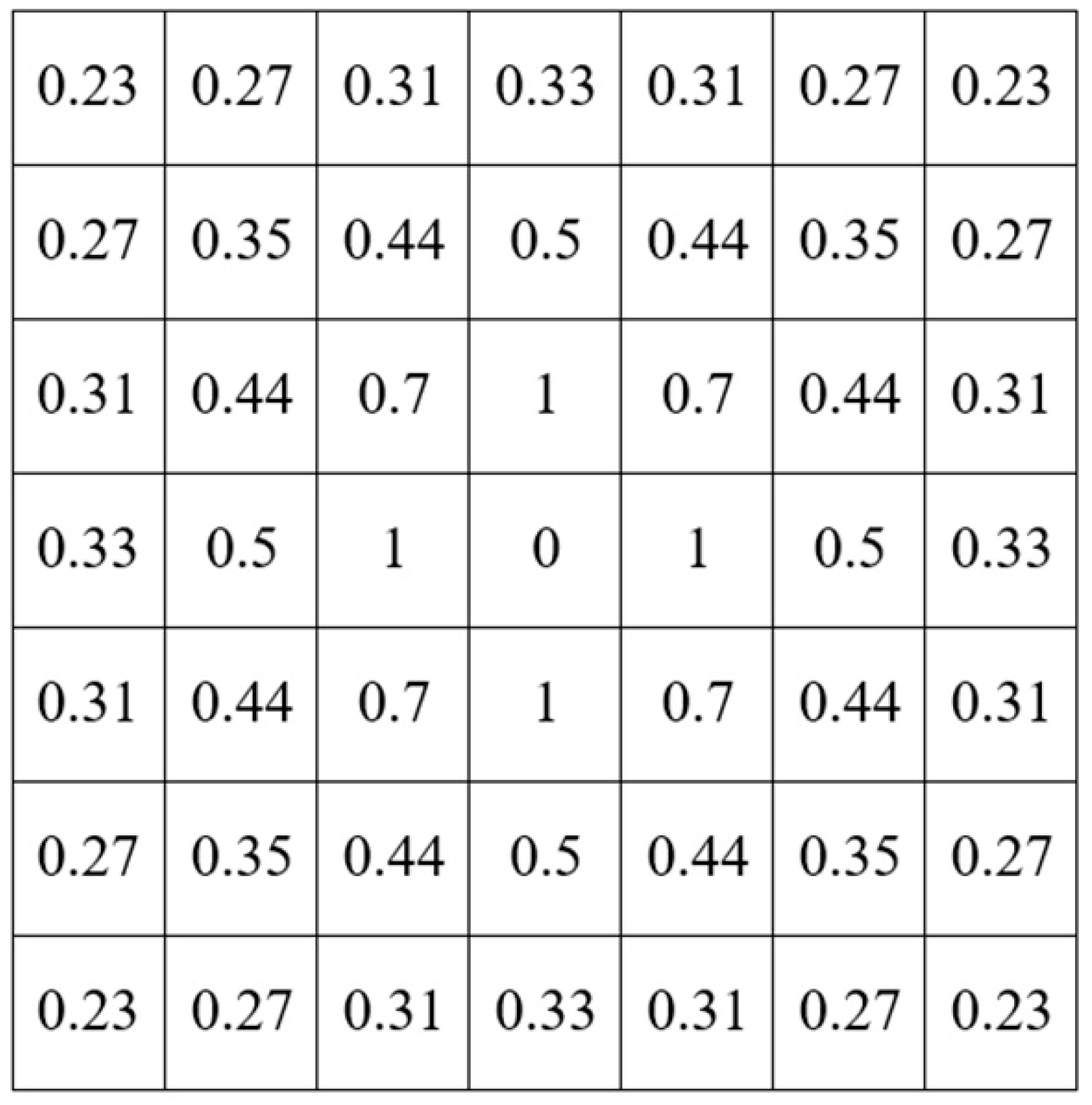
For each pixel, evidence is aggregated from neighboring pixels using a 7 × 7 weighted kernel neighborhood. The weights are determined by the inverse distance between the target pixel and each neighboring pixel. Using these weights, the belief and disbelief values for pixel i are computed as:
B F i = ( τ S A i B F + m = 1 7 n = 1 7 w m n τ S A m n B F ) / 2
D B F i = ( τ S A i D B F + m = 1 7 n = 1 7 w m n τ S A m n D B F ) / 2
where τ S A i B F and τ S A i D B F denote the membership degrees of pixel i in the belief and disbelief functions, respectively (further elaborated in the subsequent section), and w m n represents the weight assigned to the neighboring pixel located at indices (m, n) relative to pixel i (as illustrated in Figure 2). The indices m and n refer to the row and column positions of the neighboring pixels in the kernel matrix. The uncertainty for each pixel is computed using Equation (11):
U c i = 1 ( B F i + D B F i )

3.3.4. Membership Functions for Accessibility Evaluation

To classify pixels into high or low accessibility, fuzzy membership functions are applied. Specifically, the S-function (Equation (12)) is utilized for high accessibility, while the Z-function (Equation (13)) is employed for low accessibility. The choice of the S- and Z-functions is motivated by their ability to model smooth and monotonic transitions. Specifically, the S-function is well-suited for representing gradual increases toward high accessibility, while the Z-function effectively captures gradual decreases toward low accessibility. The threshold parameters are anchored to the mean (μ) and standard deviation (σ) of the accessibility values, ensuring that the membership functions adapt to the statistical distribution of the data. This design avoids abrupt binary splits and better reflects the continuous nature of spatial accessibility variations, effectively addressing the inherent ambiguity in the data.
τ S A i B F = 2 ( S A i μ + σ ) 2 , 0 S A i μ + σ 2 1 2 ( S A i ( μ + σ ) μ + σ ) 2 , μ + σ 2 S A i μ + σ 1 , S A i μ + σ
τ S A i D B F = 1 2 ( S A i μ ) 2 , 0 S A i μ 2 2 ( S A i μ μ ) 2 , μ 2 S A i μ 0 S A i μ
where τ S A i B F and τ S A i D B F represent the membership degree of pixel i in the belief and disbelief functions, respectively, and S A i denotes the spatial accessibility of the pixel i. After determining the membership degree of each pixel for high and low accessibility, the belief and disbelief values of each pixel are calculated by considering both the membership degree of the pixel itself and the neighboring pixels.
Fuzzy Set Theory (FST) is employed to manage ambiguity and gradual transitions inherent in spatial accessibility data. Traditional binary classifications often oversimplify spatial variations by enforcing rigid thresholds, whereas FST assigns degrees of membership to each area, reflecting the accessibility spectrum more accurately [44]. This approach closely mirrors real-world spatial data, which often includes inconsistencies, gaps, or continuous variations. In practice, the membership degrees obtained from the fuzzy S- and Z-functions are used to represent levels of high and low accessibility for each pixel, and these values are subsequently incorporated into the DST framework as input parameters for belief and disbelief calculations. In this way, FST provides graded membership values, while DST aggregates them across neighboring pixels to refine the final accessibility assessment.
The integration of FST with Dempster–Shafer theory (DST) enhances the analytical framework by combining their strengths. While FST models gradual transitions, DST integrates evidence from neighboring pixels, leveraging belief, disbelief, and uncertainty functions to refine accessibility assessments [41]. Together, these methodologies enable a comprehensive evaluation of spatial patterns, capturing subtle regional variations and modeling complex interactions.
By addressing variability and uncertainty in spatial accessibility data, this hybrid framework offers actionable insights for urban planning and resource allocation. It improves the robustness of accessibility evaluations, supports equitable urban development, and facilitates targeted interventions in areas with ambiguous accessibility levels, ensuring a more inclusive and sustainable approach to spatial planning.

3.4. Potential and Revealed Accessibility Maps

Upon preparing the potential and revealed accessibility maps for each category, the corresponding belief, disbelief, and uncertainty maps are generated and subsequently compared. Lower uncertainty in a region indicates that the calculated parameter in that region is more reliable [45]. Therefore, the weighted average of the revealed and potential belief values, where the weight is inversely proportional to the uncertainty value, is used to derive the final belief value for each pixel (Equation (14)) and to create a map of areas with high spatial accessibility.
Similarly, the weighted average of the disbelief values from the potential and revealed maps is utilized to determine the final disbelief value for each pixel (Equation (15)) and to generate the map of areas with low spatial accessibility. This approach ensures that areas with lower uncertainty contribute more significantly to the final belief and disbelief values, thereby enhancing the reliability of the spatial accessibility assessment.
F i n a l B F i = w i ( r ) B F i ( r ) + w i ( e ) B F i ( e ) w i ( r ) + w i ( e )
F i n a l D B F i = w i ( r ) D B F i ( r ) + w i ( e ) D B F i ( e ) w i ( r ) + w i ( e )
where B F i ( r ) is the revealed belief value of pixel i, B F i ( e ) is the potential belief value of pixel i, D B F i ( r ) is the revealed disbelief value of pixel i, and D B F i ( e ) is the potential disbelief value of pixel i. Additionally, w i ( r ) is the revealed weight of pixel i and w i ( e ) is the potential weight of pixel i, which are obtained using the following equations:
w i ( r ) = 1 U c i ( r ) 2
w i ( e ) = 1 U c i ( e ) 2
where U c i ( r ) is the revealed uncertainty of pixel i and U c i ( e ) is the potential uncertainty of pixel i.

4. Data and Study Area

The Canton of Vaud, Switzerland, was selected as the study area for implementing the proposed method. Mobile Data Challenge (MDC) data were utilized to prepare the revealed accessibility map, while Point of Interest (POI) data retrieved from OpenStreetMap (OSM) were employed to prepare the potential accessibility map.

4.1. MDC

The MDC data, related to the Lausanne Data Collection Campaign (LDCC) conducted between 2009 and 2011 around Lake Geneva, Switzerland, were used to develop the revealed accessibility map [46]. Participants from the Lake Geneva region voluntarily agreed to participate in the project, driven primarily by altruistic motives. Data were collected from 200 volunteers using Nokia N95 phones, with most participants remaining in the study for over a year [46]. The participant demographic attributes included gender (62% were men, 38% were women), age group (a. 16–21, b. 22–27, c. 28–33, d. 33–38, e. 39–44, f. 45–50, g. over 50 years old), and job type (working full-time, working part-time, not currently working, studying full-time, studying part-time, and stay-at-home partner).
The data collected encompassed location (GPS), communications (phone calls and text messages), among others. Additionally, participants specified the areas they visited by partaking in a semantic tag survey. Stopping locations were initially determined using the method presented [42], after which participants assigned labels to each of the predefined categories for places (home, workplace, shop, restaurant, sports center, etc.). For this research, data from the Canton of Vaud were selected. Origin–destination (OD) data were constructed using GPS points recorded every 5 s and stop point data (as described in Section 3.2). After categorizing OD data based on destination type, categories with an acceptable number of records were chosen: shops, sports centers, and restaurants. There were 6345, 1275, and 1558 OD records with destinations at shops, sports centers, and restaurants, respectively (Figure 3).
To ensure the accuracy of the data, a map matching technique was employed. This method involved using the proximity to road segments parameter on 30% of the dataset to validate the GPS data points against known road networks. This process enhanced the reliability of the revealed accessibility map by ensuring that the recorded movements accurately reflected real-world travel paths.

4.2. OSM

The Overpass API (Overpass API: https://overpass-turbo.eu/, accessed on 21 November 2023) was utilized to download the OSM data necessary for preparing the potential accessibility map. Points of Interest (POIs) as of the end of 2011, related to the categories of shops, sports centers, and restaurants, were downloaded. In the Canton of Vaud, there are 583 restaurants, 584 shops, and 150 sports centers (Figure 4a). Additionally, the road network data required for determining the access range in both the potential and revealed accessibility maps were obtained from the OSM website to form the road network (Figure 4b). Population data for the target area, corresponding to the year 2009, at a 1 × 1 km grid resolution, were downloaded from the “WorldPop” (WorldPop: https://hub.worldpop.org, accessed on 21 November 2023) website (Figure 4c).

5. Results and Discussion

In this study, supply centers were selected from the following categories: shops, restaurants, and sports centers (as explained in Section 4.1). The potential accessibility map was prepared using the Enhanced Two-Step Floating Catchment Area (E2SFCA) method, employing weights of 1.00, 0.68, and 0.22 for the three travel time zones. These weights were adopted from previous studies applying the E2SFCA method [31] and reflect the gradual distance decay effect on accessibility. To ensure consistency and meaningful comparison between potential and revealed accessibility, all values are normalized to a [0, 1] range using the min–max normalization method. The choropleth maps in Figure 5 and subsequent figures are classified using the Jenks natural breaks method, which minimizes within-class variance and maximizes between-class contrast, making it well-suited for the skewed distribution of accessibility values. While the overall spatial patterns remain consistent, alternative schemes (e.g., equal interval or quantiles) could shift class boundaries, potentially emphasizing the different areas as high- or low-access areas and thereby influencing policy interpretations. Figure 5 displays the potential and revealed accessibility maps for the datasets corresponding to shops, restaurants, and sports centers. Areas with an access value lower than μ 3 σ are considered to have low accessibility, while those with values above the μ + 3 σ are considered to have high accessibility. This threshold follows the empirical three-sigma rule, where values beyond μ ± 3 σ are statistically rare, providing an objective criterion for classifying low and high accessibility.
The highest mean and standard deviation in the potential accessibility maps are observed for shops, while sports centers have the lowest mean, and restaurants have the lowest standard deviation of PA (Table 1). Among the ten cities of the Canton of Vaud, the central parts of Aigle demonstrate good potential access to all supply centers. Additionally, Riviera-Pays-d’Enhaut exhibits the best potential access to shops. Apart from these areas, the central region of the canton exhibits better potential access to restaurants and shops.
In the revealed accessibility maps, restaurants and shops have the highest and lowest RA means and standard deviations, respectively. In contrast to the potential maps, the city of Aigle demonstrates low access to all supply centers in the revealed maps. Areas proximate to Lake Geneva exhibit high revealed access to shops, and most areas with high revealed access to restaurants are located in Jura-Nord Vaudois. Broye-Vully and the eastern parts of Lavaux-Oron exhibit high revealed access to sports centers.
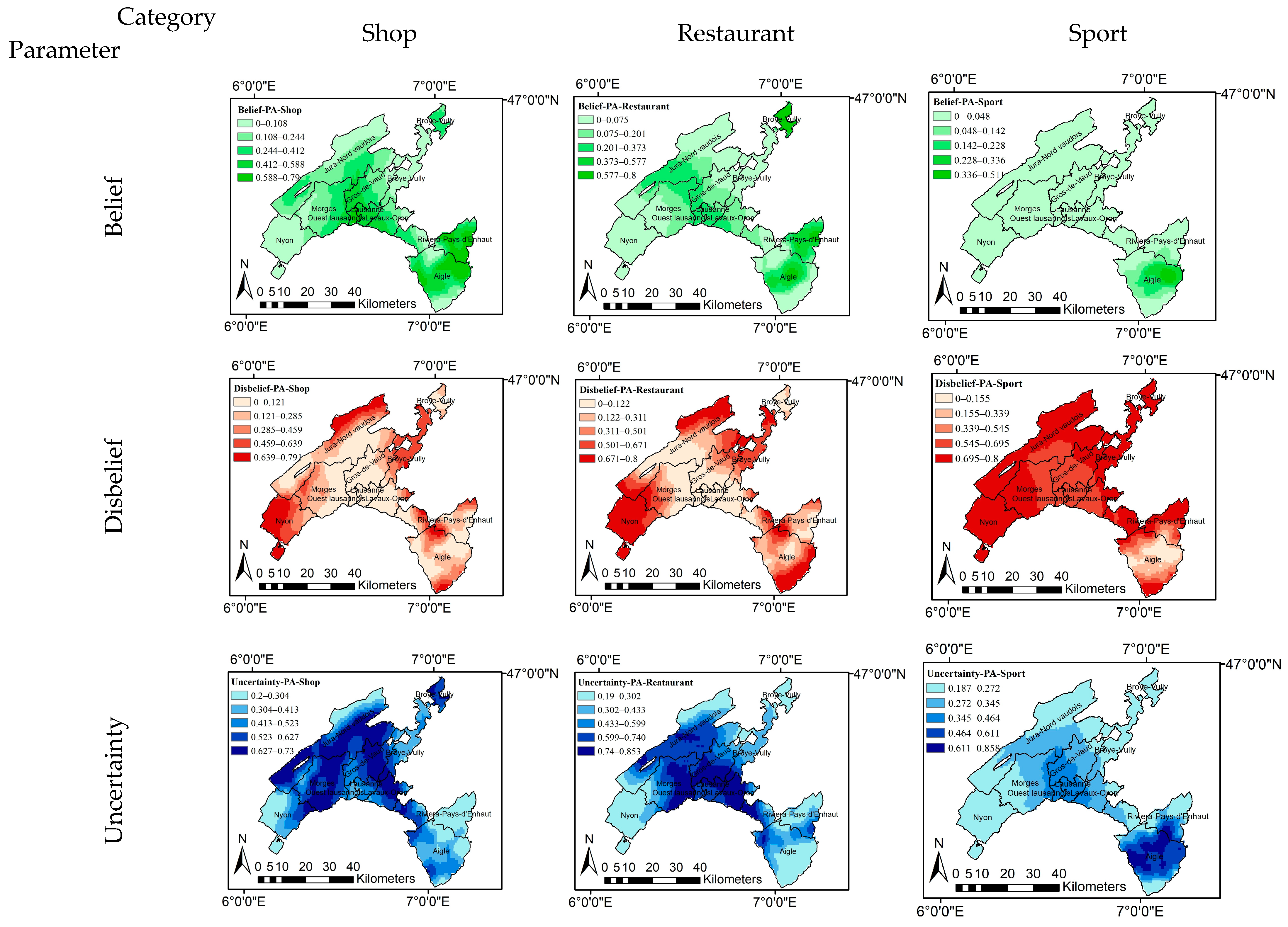
Figure 6 illustrates the belief, disbelief, and uncertainty maps for potential spatial accessibility. Comparing the potential accessibility belief maps across all categories with the corresponding disbelief maps reveals that areas with moderate–high belief levels are correlated with areas of low disbelief (Figure 7), indicating that areas with high belief in potential accessibility coincide with areas of low disbelief in potential accessibility.
Comparing the belief map of potential accessibility for the shop category with the uncertainty map of potential accessibility reveals that areas with high belief levels are correlated with areas of low uncertainty (Figure 8a). Consequently, belief in high potential accessibility is considered reliable in these areas.
For the restaurant category in the eastern cities (Broye-Vully, Riviera-Pays-d’Enhaut, and Aigle), areas with high potential belief exhibit low uncertainty (Figure 8b). However, the central regions, despite having high belief levels, exhibit high uncertainty, rendering belief in high accessibility unreliable in these areas.
For the sports category, comparing the potential belief map with the uncertainty map reveals that areas with moderate–high belief levels are correlated with areas of high uncertainty (Figure 8c). Therefore, belief in high accessibility is deemed unreliable in these areas. Additionally, the disbelief map is correlated with the uncertainty map, indicating that areas with low disbelief exhibit high uncertainty (Figure 6).
Figure 9 illustrates the belief, disbelief, and uncertainty maps for revealed spatial accessibility across all categories. Comparing the belief maps of revealed spatial accessibility with the disbelief maps demonstrates that areas with moderate–high belief levels are correlated with areas of low disbelief (Figure 10). This complementarity indicates that disbelief maps enhanced belief maps, with areas of low disbelief coinciding with areas of high belief. The uncertainty map, displaying relatively low uncertainty for areas with moderate–high belief, indicates that belief in high accessibility was reliable in these areas (Figure 11).
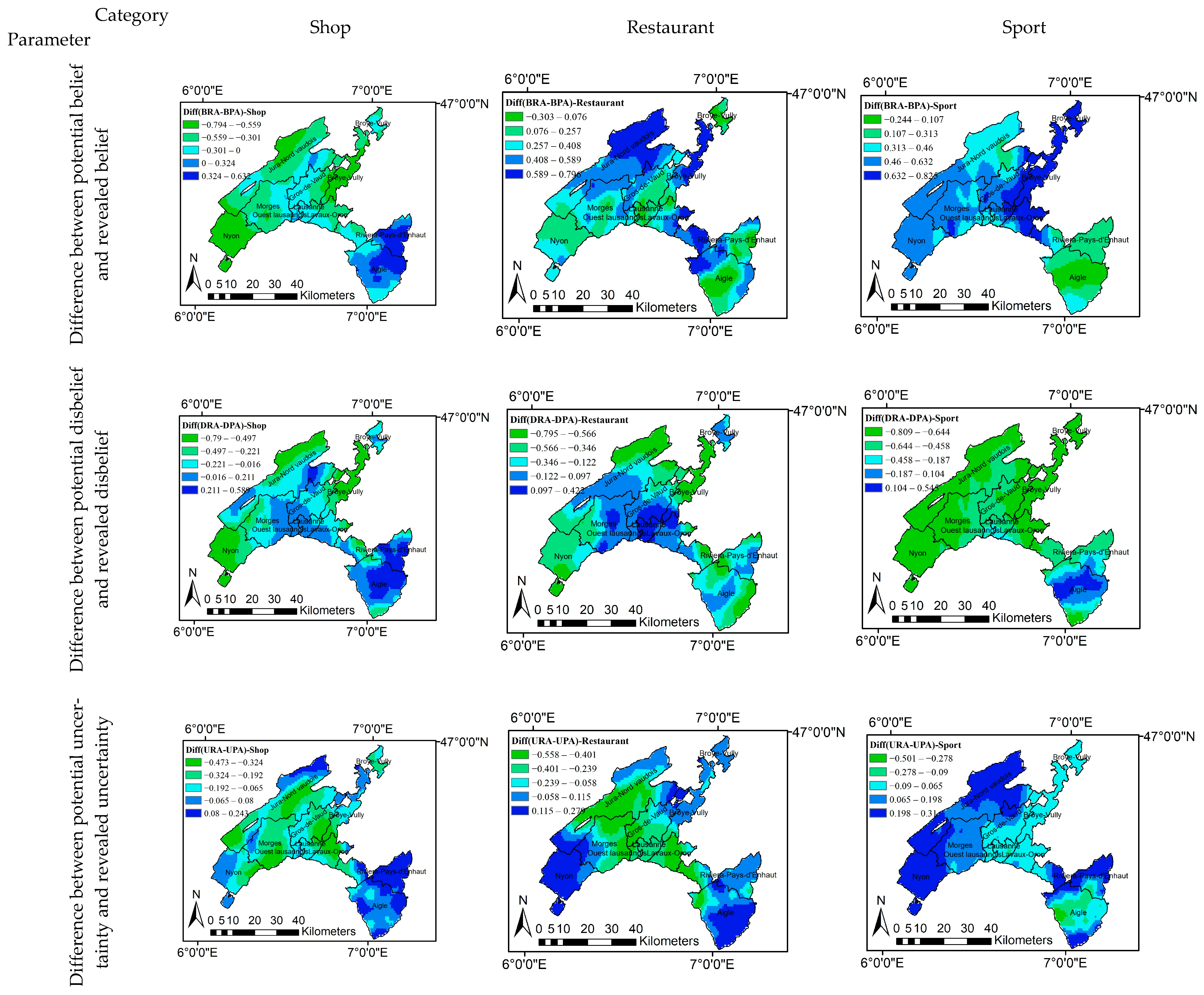
Figure 12 highlights the differences between the belief, disbelief, and uncertainty maps of revealed and potential accessibility. For the shop category, the revealed belief in most areas is lower than the potential belief, suggesting that real-world spatial accessibility to shops was less than the potential value. Conversely, for the restaurant and sports center categories, the revealed accessibility belief was higher than the potential belief, indicating that individuals’ spatial accessibility is greater in reality.
In all categories, the revealed disbelief is lower than the potential disbelief in most regions, suggesting that real-world areas have lower accessibility than potential values. In the uncertainty maps for the shop and restaurant categories, the revealed uncertainty was lower than the potential uncertainty in most regions, indicating that revealed maps are more reliable than potential maps in most cases. However, for sports centers, the potential uncertainty is lower than the revealed uncertainty in most areas, suggesting that potential maps are more reliable than revealed maps.
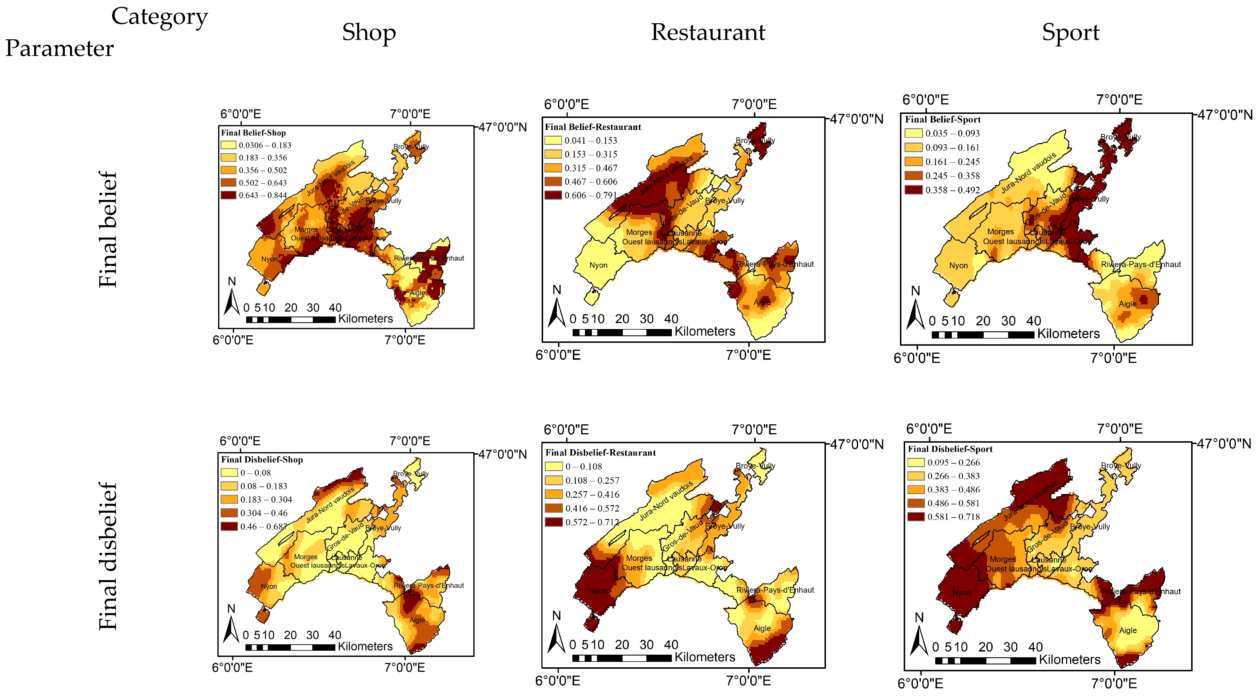
The final belief map is derived from the weighted average of the revealed and potential belief values, while the final disbelief map is derived from the weighted average of the revealed and potential disbelief values (Figure 13). In the final belief map, darker areas indicate high accessibility, whereas in the final disbelief map, darker areas indicate poor accessibility. These darker zones in the disbelief maps (Figure 13) are directly considered as shortage regions, and their areal extent forms the basis for the percentages reported in Table 2. Across all categories, the final belief and disbelief maps are complementary, with areas of high belief corresponding to low disbelief (Figure 14). Generally, areas with low access to sports centers have the highest percentage, followed by restaurants and shops (Table 2).
Most parts of the Canton of Vaud exhibit good access to shops, with parts of Aigle and northern Jura-Nord Vaudois demonstrating the lowest access. The northeastern parts of Lake Geneva, Jura-Nord Vaudois, and northeastern Broye-Vully exhibit good access to restaurants, while Nyon and southern Aigle have the lowest access. Most of the Canton of Vaud exhibits poor access to sports centers, with Nyon, Jura-Nord Vaudois, and Riviera-Pays-d’Enhaut demonstrating the lowest access, and Broye-Vully and Lavaux-Oron demonstrating the best access.
The integration of potential and revealed accessibility maps using the Dempster–Shafer theory provides a robust framework for urban planning decisions. By explicitly modeling uncertainty, planners can distinguish areas where accessibility assessments are reliable from those requiring additional data or investment. For example, the high disbelief and uncertainty in access to sports centers in Nyon and Jura-Nord Vaudois indicate not only a shortage of facilities but also a misalignment between existing infrastructure and users’ behavioral patterns. These insights can inform planning by highlighting where resources should be prioritized and by linking accessibility evaluation more directly to policy objectives of spatial equity.
In summary, the analysis of potential and revealed accessibility maps, alongside the belief, disbelief, and uncertainty maps, provides a comprehensive understanding of spatial accessibility across different supply categories within the canton of Vaud. The findings highlight significant variations in accessibility and reliability across shops, restaurants, and sports centers. To further contextualize these insights, the subsequent section delves into the relationship between station density, population density, and the discrepancies in belief values. Additionally, it examines the correlation between station density, population density, and uncertainty of real accessibility, offering a deeper understanding of the factors influencing spatial accessibility. This detailed examination offers further perspectives on the complexities of managing accessibility and underscores the need for tailored strategies in different density contexts.
Figure 15 illustrates the relationship between station density (i.e., stations per kilometer) and the absolute difference between observed and expected belief values (ABS (Bel Real—Bel Exp)) across three land use categories: shops, restaurants, and sports centers. To assess the statistical significance of these relationships, Pearson correlation tests are applied, and the corresponding p-values are reported. Statistically significant positive correlations were found for shops (p = 1.3 × 10⁻³¹) and restaurants (p = 6.17 × 10⁻¹³), indicating that higher station densities are associated with greater discrepancies between actual and perceived accessibility. In these categories, most station densities are below 10 stations per kilometer, where smaller belief differences are observed. In contrast, the sports centers category does not exhibit a statistically significant relationship (p = 0.57), suggesting that station density does not meaningfully impact belief discrepancies in this context. These findings highlight the importance of targeted planning in high-density areas, especially for shops and restaurants, to reduce mismatches between real and perceived accessibility.
Figure 16 illustrates the relationship between station density (measured in stations per kilometer) and real uncertainty values in belief data across three land use categories: shops, restaurants, and sports centers. The scatter plots show that most data points cluster around lower uncertainty levels (0.2 to 0.4), generally indicating low–moderate uncertainty. Statistically significant relationships are observed across all categories, with p-values of 1.3 × 10⁻³¹ for shops, 6.17 × 10⁻¹³ for restaurants, and 9.18 × 10⁻¹¹ for sports centers. In shops and restaurants, station densities predominantly remain below 10 stations per kilometer, suggesting that lower station densities are associated with reduced uncertainty in belief data. Conversely, the sports category exhibits a broader distribution of both station densities and uncertainty values, including outliers above 40 stations per kilometer and uncertainty levels approaching 0.6. This pattern indicates that higher station densities, especially in sports centers, correspond to increased uncertainty in belief measurements. These findings underscore the necessity for targeted approaches to effectively manage uncertainty in high-density urban areas, thereby enhancing the accuracy and reliability of spatial accessibility assessments.
Figure 17 illustrates the relationship between population density (measured in population per square kilometer) and the absolute difference between observed and expected belief values (ABS (Bel Real—Bel Exp)) across three land use categories: shops, restaurants, and sports centers. Statistically significant associations are observed for shops (p = 4.3 × 10⁻²⁹) and sports centers (p = 1.16 × 10⁻⁹), indicating that higher population densities tend to be associated with smaller discrepancies between actual and perceived accessibility in these categories. Conversely, the relationship for restaurants is not statistically significant (p = 0.99), suggesting that population density does not meaningfully explain the belief differences in this category. The scatter plots reveal that shops and restaurants generally experience smaller belief discrepancies at higher population densities, implying effective spatial planning and service distribution. Sports centers display greater variability in both population density and belief differences, highlighting the complexity of factors influencing accessibility perceptions in this category. These findings underscore the need to incorporate population density considerations into spatial accessibility assessments to promote equitable and reliable access across diverse urban contexts.
Figure 18 depicts the relationship between population density (measured in population per square kilometer) and real uncertainty in belief values across three land use categories: shops, restaurants, and sports centers. Statistically significant relationships are observed for shops (p = 4.29 × 10⁻¹⁷) and restaurants (p = 1.29 × 10⁻¹²), indicating that higher population densities are associated with lower uncertainty in belief data within these categories. Most data points for shops and restaurants cluster within lower uncertainty ranges (0.2 to 0.4), with population densities generally below 3000 people per square kilometer, suggesting consistent and reliable belief values in moderately populated areas. Conversely, the sports centers category exhibits a broader distribution of population densities and uncertainty values, including several outliers with population densities reaching up to 7000 people per square kilometer and uncertainty levels up to 0.6. Although the p-value for sports centers (p = 2.19 × 10⁻⁸) indicates a statistically significant relationship, the greater variability suggests more complex factors influencing uncertainty in this category. These findings highlight the importance of developing targeted strategies to manage uncertainty in highly populated areas, particularly for sports centers, to enhance the accuracy and reliability of spatial accessibility assessments.
This study’s comparative analysis between potential and revealed accessibility surfaces, supported by belief, disbelief, and uncertainty metrics, revealed both alignments and notable divergences across service categories. The revealed accessibility maps, especially for restaurants and sports centers, often indicate higher actual access than predicted, emphasizing the importance of incorporating behavior-based data in accessibility assessments. This demonstrates that relying solely on infrastructure-based models may underestimate individuals’ real-world spatial experiences. Furthermore, areas with higher population or station density exhibited lower uncertainty and belief discrepancies, confirming the stabilizing effect of infrastructure density on accessibility perceptions.
Although this study focused on the Canton of Vaud, the proposed methodology is broadly applicable to other urban or regional contexts, provided that comparable datasets, such as population grids, points of interest, road networks, and mobility traces, are available. However, the generalizability of the results may be influenced by regional differences in mobility behavior, data quality, and service classification standards. Therefore, future applications should carefully adapt input parameters and accessibility thresholds to local conditions to ensure methodological consistency and relevance.

6. Conclusions

This research introduced a novel framework integrating revealed and potential accessibility maps using the Dempster–Shafer theory to address uncertainty in spatial accessibility. Applying this method to shops, restaurants, and sports centers in the Canton of Vaud, Switzerland, demonstrated a comprehensive approach to accessibility evaluation.
Potential accessibility maps, created with the Enhanced Two-Step Floating Catchment Area (E2SFCA) method, showed that shops generally had the highest potential accessibility, while sports centers had the lowest. However, revealed accessibility maps based on actual movement data indicated that restaurants had the highest practical accessibility, highlighting differences between modeled and real-world access.
Beyond its technical formulation, the DST-based uncertainty maps provide practical insights for urban planning. For example, areas with high disbelief and low uncertainty can be prioritized for new facilities, such as sports centers or clinics, since the evidence of poor access is more reliable. Conversely, areas with high uncertainty reveal data gaps and highlight the need for further surveys or participatory assessments before making planning decisions. By distinguishing reliable evidence from unreliable evidence, DST enables more transparent and defensible allocation of community resources. However, its effectiveness still depends on the availability of representative input data, which may vary across regions. Recognizing these limitations is essential if we are to avoid over-reliance on technical outputs and to ensure that DST functions as a complementary decision-support tool.
Station and population density influenced accessibility patterns: higher densities correlated with lower uncertainty and smaller discrepancies between expected and revealed accessibility, emphasizing their stabilizing effects.
Integrating potential and revealed maps ensures planning decisions reflect both theoretical models and actual usage patterns, increasing map reliability compared to traditional methods focused only on population and travel cost. This approach also accounts for personal preferences, service quality, and other factors affecting access.
Additionally, the E2SFCA method presents limitations, particularly in its limited consideration of demand-side factors and temporal variability. Incorporating dynamic temporal models and advanced interpolation techniques, such as kriging or machine learning, could enhance both the accuracy and comprehensiveness of accessibility assessments. The use of IDW interpolation, while methodologically straightforward, also introduces constraints: it assumes spatial correlation is determined solely by distance and is highly sensitive to data density. This may reduce accuracy in areas with sparse OD records, such as rural regions. More sophisticated network-based or geostatistical interpolation methods could help mitigate these limitations in future studies and practical applications.
Another limitation is the uniform treatment of facility service capacity. Differences in the size or capacity of stores, restaurants, and sports centers were not accounted for, potentially oversimplifying accessibility evaluations. Furthermore, while the framework is methodologically robust, it does not yet incorporate diverse transportation modes, which significantly influence accessibility. The unimodal focus on driving time overlooks the role of walking, cycling, and public transit—modes particularly relevant for elderly and low-income populations. This simplification may lead to an overestimation of accessibility for certain groups and reduce the practical relevance of planning recommendations. Future research should extend the framework to include multimodal datasets to better capture differential mobility patterns.
Finally, this study relies on the MDC dataset collected from 200 volunteers, which may not fully represent the population of the canton of Vaud. Consequently, accessibility patterns of certain groups, such as the elderly, gender groups, or low-income populations, might be underrepresented. We also acknowledge that the limited geographic distribution of participants may lead to artificial hotspots in sparsely sampled areas. While advanced approaches such as bootstrapping or Monte Carlo simulations were not applied here, they represent valuable directions for future research to better address data bias and quantify uncertainty. In addition, the timeliness of the datasets poses another limitation, as the MDC trajectories (2009–2011), POI data (2011), and population data (2009) may not fully capture more recent changes in facility distribution, mobility patterns, or transport networks. Nonetheless, since the main objective of this study was to propose and test a methodological framework, these datasets remain suitable for demonstrating the approach. Future research should employ larger, more representative, and up-to-date multi-period datasets to enhance generalizability and validate the stability of the weighting indicators.

Author Contributions

Conceptualization, Roya Esmaeili Tajabadi and Amin Hosseinpoor Milaghardan; methodology, Roya Esmaeili Tajabadi and Amin Hosseinpoor Milaghardan; software, Roya Esmaeili Tajabadi; validation, Roya Esmaeili Tajabadi, Parham Pahlavani, Amin Hosseinpoor Milaghardan and Christophe Claramunt; formal analysis, Roya Esmaeili Tajabadi; investigation, Roya Esmaeili Tajabadi; data curation, Roya Esmaeili Tajabadi; writing—original draft preparation, Roya Esmaeili Tajabadi; writing—review and editing, Roya Esmaeili Tajabadi, Parham Pahlavani, Amin Hosseinpoor Milaghardan and Christophe Claramunt; visualization, Roya Esmaeili Tajabadi; supervision, Parham Pahlavani; project administration, Parham Pahlavani. All authors have read and agreed to the published version of the manuscript.

Funding

This research received no external funding.

Data Availability Statement

The MDC dataset is available here: https://www.idiap.ch/en/dataset/mdc (accessed on 15 August 2025). The data are not public, but are available to eligible institutions.

Acknowledgments

The authors would like to thank LDCC for providing access to the MDC dataset.

Conflicts of Interest

The authors declare that they have no known competing financial interests or personal relationships that could have appeared to influence the work reported in this paper.

References

  1. The United Nations Department of Economic and Social Affairs (UN DESA). World Urbanization Prospects, The 2014 Revision; United Nations: New York, NY, USA, 2014. [Google Scholar]
  2. Van Maarseveen, M.; Martinez, J.; Flacke, J. GIS in Sustainable Urban Planning and Management: A Global Perspective; Taylor & Francis: Abingdon, UK, 2019. [Google Scholar]
  3. Wang, F.; Luo, W. Assessing spatial and nonspatial factors for healthcare access: Towards an integrated approach to defining health professional shortage areas. Health Place 2005, 11, 131–146. [Google Scholar] [CrossRef] [PubMed]
  4. Ashik, F.R.; Mim, S.A.; Neema, M.N. Towards vertical spatial equity of urban facilities: An integration of spatial and aspatial accessibility. J. Urban Manag. 2020, 9, 77–92. [Google Scholar] [CrossRef]
  5. Park, J.; Goldberg, D.W. A review of recent spatial accessibility studies that benefitted from advanced geospatial information: Multimodal transportation and spatiotemporal disaggregation. ISPRS Int. J. Geo-Inf. 2021, 10, 532. [Google Scholar] [CrossRef]
  6. Geurs, K.T.; Van Wee, B. Accessibility evaluation of land-use and transport strategies: Review and research directions. J. Transp. Geogr. 2004, 12, 127–140. [Google Scholar] [CrossRef]
  7. Hewko, J.; Smoyer-Tomic, K.E.; Hodgson, M.J. Measuring neighbourhood spatial accessibility to urban amenities: Does aggregation error matter? Environ. Plan. A 2002, 34, 1185–1206. [Google Scholar] [CrossRef]
  8. Guagliardo, M.F. Spatial accessibility of primary care: Concepts, methods and challenges. Int. J. Health Geogr. 2004, 3, 3. [Google Scholar] [CrossRef]
  9. Apparicio, P.; Abdelmajid, M.; Riva, M.; Shearmur, R. Comparing alternative approaches to measuring the geographical accessibility of urban health services: Distance types and aggregation-error issues. Int. J. Health Geogr. 2008, 7, 7. [Google Scholar] [CrossRef]
  10. Smoyer-Tomic, K.E.; Hewko, J.N.; Hodgson, M.J. Spatial accessibility and equity of playgrounds in Edmonton, Canada. Can. Geogr./Géographies Can. 2004, 48, 287–302. [Google Scholar] [CrossRef]
  11. Smoyer-Tomic, K.E.; Spence, J.C.; Amrhein, C. Food deserts in the prairies? Supermarket accessibility and neighborhood need in Edmonton, Canada. Prof. Geogr. 2006, 58, 307–326. [Google Scholar] [CrossRef]
  12. Janatabadi, F.; Newing, A.; Ermagun, A. Social and spatial inequalities of contemporary food deserts: A compound of store and online access to food in the United Kingdom. Appl. Geogr. 2024, 163, 103184. [Google Scholar] [CrossRef]
  13. Rao, Y.; Zhong, Y.; He, Q.; Dai, J. Assessing the Equity of Accessibility to Urban Green Space: A Study of 254 Cities in China. Int. J. Environ. Res. Public Health 2022, 19, 4855. [Google Scholar] [CrossRef]
  14. Wang, L. Immigration, ethnicity, and accessibility to culturally diverse family physicians. Health Place 2007, 13, 656–671. [Google Scholar] [CrossRef] [PubMed]
  15. Wang, J.; Du, F.; Huang, J.; Liu, Y. Access to hospitals: Potential vs. observed. Cities 2020, 100, 102671. [Google Scholar] [CrossRef]
  16. Lin, S.-J.; Crawford, S.Y.; Salmon, J.W. Potential access and revealed access to pain management medications. Soc. Sci. Med. 2005, 60, 1881–1891. [Google Scholar] [CrossRef]
  17. Pot, F.J.; van Wee, B.; Tillema, T. Perceived accessibility: What it is and why it differs from calculated accessibility measures based on spatial data. J. Transp. Geogr. 2021, 94, 103090. [Google Scholar] [CrossRef]
  18. Chen, B.Y.; Yuan, H.; Li, Q.; Wang, D.; Shaw, S.-L.; Chen, H.-P.; Lam, W.H. Measuring place-based accessibility under travel time uncertainty. Int. J. Geogr. Inf. Sci. 2017, 31, 783–804. [Google Scholar] [CrossRef]
  19. Schiewe, J.; Knura, M. Consideration of uncertainty information in accessibility analyses for an effective use of urban infrastructures. ISPRS Int. J. Geo-Inf. 2021, 10, 171. [Google Scholar] [CrossRef]
  20. Conway, M.W.; Byrd, A.; Van Eggermond, M. Accounting for uncertainty and variation in accessibility metrics for public transport sketch planning. J. Transp. Land Use 2018, 11, 541–558. [Google Scholar] [CrossRef]
  21. Hansen, W.G. How accessibility shapes land use. J. Am. Inst. Plan. 1959, 25, 73–76. [Google Scholar] [CrossRef]
  22. Dalvi, M.Q.; Martin, K. The measurement of accessibility: Some preliminary results. Transportation 1976, 5, 17–42. [Google Scholar] [CrossRef]
  23. Patterson, Z.; Farber, S. Potential path areas and activity spaces in application: A review. Transp. Rev. 2015, 35, 679–700. [Google Scholar] [CrossRef]
  24. O’Kelly, M.E.; Horner, M.W. Aggregate accessibility to population at the county level: US 1940–2000. J. Geogr. Syst. 2003, 5, 5–23. [Google Scholar] [CrossRef]
  25. Miller, E.J. Accessibility: Measurement and application in transportation planning. Transp. Rev. 2018, 38, 551–555. [Google Scholar] [CrossRef]
  26. Van Wee, B. Accessible accessibility research challenges. J. Transp. Geogr. 2016, 51, 9–16. [Google Scholar] [CrossRef]
  27. Dai, D.; Wang, F. Geographic disparities in accessibility to food stores in southwest Mississippi. Environ. Plan. B Plan. Des. 2011, 38, 659–677. [Google Scholar] [CrossRef]
  28. Wu, H.; Levinson, D. Unifying access. Transp. Res. Part D Transp. Environ. 2020, 83, 102355. [Google Scholar] [CrossRef]
  29. Radke, J.; Mu, L. Spatial decompositions, modeling and mapping service regions to predict access to social programs. Geogr. Inf. Sci. 2000, 6, 105–112. [Google Scholar] [CrossRef]
  30. Luo, W.; Wang, F. Measures of spatial accessibility to health care in a GIS environment: Synthesis and a case study in the Chicago region. Environ. Plan. B Plan. Des. 2003, 30, 865–884. [Google Scholar] [CrossRef]
  31. Luo, W.; Qi, Y. An enhanced two-step floating catchment area (E2SFCA) method for measuring spatial accessibility to primary care physicians. Health Place 2009, 15, 1100–1107. [Google Scholar] [CrossRef]
  32. Khan, A.A.; Bhardwaj, S.M. Access to health care: A conceptual framework and its relevance to health care planning. Eval. Health Prof. 1994, 17, 60–76. [Google Scholar] [CrossRef]
  33. Páez, A.; Scott, D.M.; Morency, C. Measuring accessibility: Positive and normative implementations of various accessibility indicators. J. Transp. Geogr. 2012, 25, 141–153. [Google Scholar] [CrossRef]
  34. Casas, I.; Delmelle, E.; Delmelle, E.C. Potential versus revealed access to care during a dengue fever outbreak. J. Transp. Health 2017, 4, 18–29. [Google Scholar] [CrossRef]
  35. Lättman, K.; Olsson, L.E.; Friman, M. A new approach to accessibility–Examining perceived accessibility in contrast to objectively measured accessibility in daily travel. Res. Transp. Econ. 2018, 511–501, 69. [Google Scholar] [CrossRef]
  36. Lättman, K.; Olsson, L.E.; Friman, M. Development and test of the perceived accessibility scale (PAC) in public transport. J. Transp. Geogr. 2016, 54, 257–263. [Google Scholar] [CrossRef]
  37. Friman, M.; Lättman, K.; Olsson, L.E. Public transport quality, safety, and perceived accessibility. Sustainability 2020, 12, 3563. [Google Scholar] [CrossRef]
  38. Hunter, G.J.; Goodchild, M. Managing uncertainty in spatial databases: Putting theory into practice. URISA J. 1993, 5, 55–62. [Google Scholar]
  39. Batty, M. Unpredictability. Environ. Plan. B Urban Anal. City Sci. 2020, 47, 739–744. [Google Scholar] [CrossRef]
  40. Dempster, A.P. Upper and lower probabilities induced by a multivalued mapping. Ann. Math. Stat. 1967, 325–339. [Google Scholar] [CrossRef]
  41. Shafer, G. A Mathematical Theory of Evidence; Princeton University Press: Princeton, NJ, USA, 1976; Volume 1. [Google Scholar]
  42. Montoliu, R.; Gatica-Perez, D. Discovering human places of interest from multimodal mobile phone data. In Proceedings of the 9th International Conference on Mobile and Ubiquitous Multimedia, Limassol, Cyprus, 1–3 December 2010; p. 12. [Google Scholar]
  43. Shi, W. Principles of Modeling Uncertainties in Spatial Data and Spatial Analyses; CRC Press: Boca Raton, FL, USA, 2009. [Google Scholar]
  44. Zadeh, L.A. Fuzzy sets. Inf. Control 1965, 8, 338–353. [Google Scholar] [CrossRef]
  45. Mogaji, K.; Lim, H.; Abdullah, K. Regional prediction of groundwater potential mapping in a multifaceted geology terrain using GIS-based Dempster–Shafer model. Arab. J. Geosci. 2015, 8, 3235–3258. [Google Scholar] [CrossRef]
  46. Laurila, J.K.; Gatica-Perez, D.; Aad, I.; Bornet, O.; Do, T.-M.-T.; Dousse, O.; Eberle, J.; Miettinen, M. The mobile data challenge: Big data for mobile computing research. In Proceedings of the Pervasive Computing, Newcastle, UK, 18–22 June 2012. [Google Scholar]
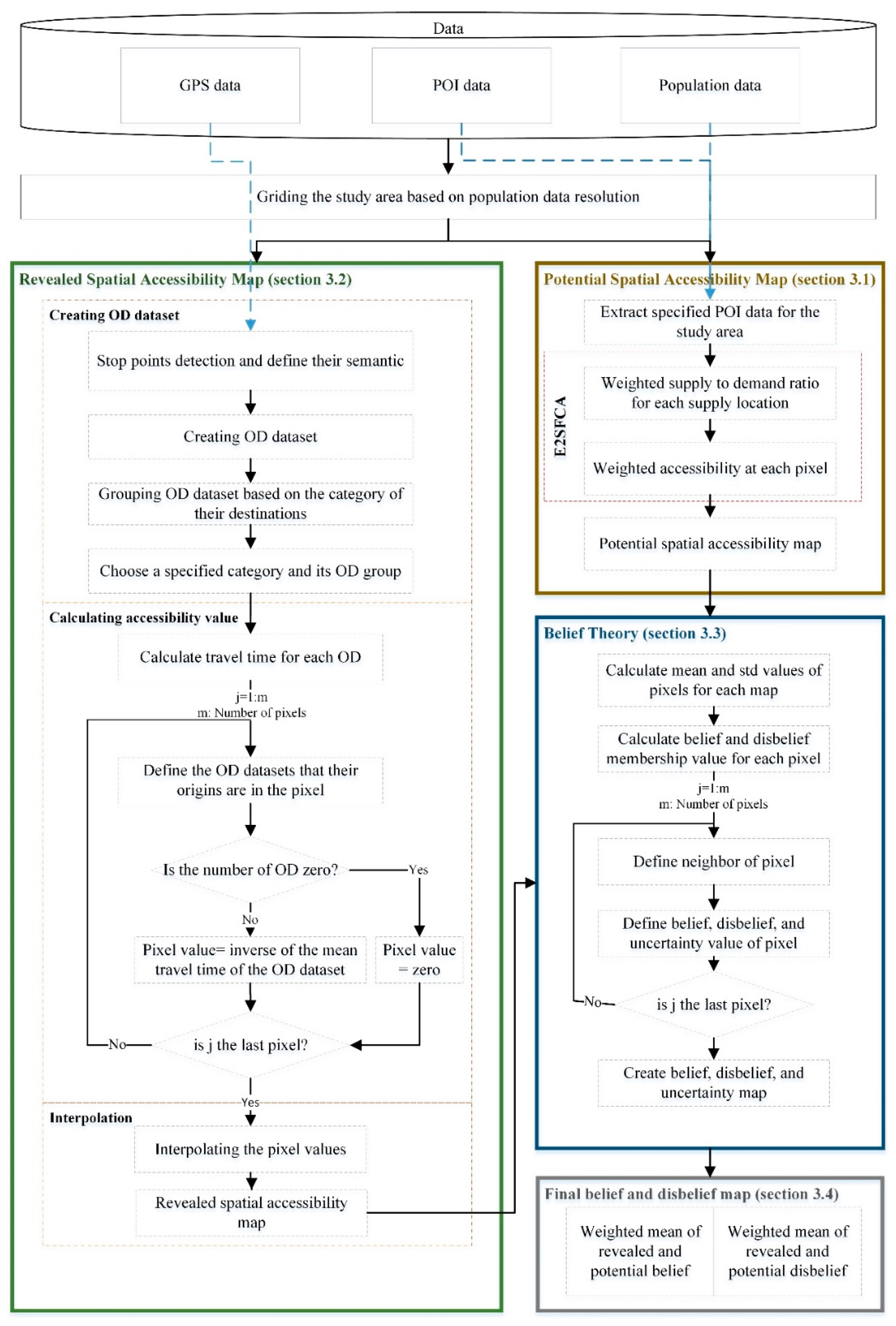
Figure 1. Proposed method.
Ijgi 14 00370 g001
Figure 2. Neighborhood weights for calculating belief and disbelief of each pixel.
Ijgi 14 00370 g002
Figure 3. Origins of OD data. Three destination categories are (a) shop, (b) restaurant, and (c) sport.
Ijgi 14 00370 g003
Figure 4. (a) OSM POIs in shop, sport, and restaurant categories; (b) road networks; (c) population density in 2009 with 1 km × 1 km grid.
Ijgi 14 00370 g004
Figure 5. Potential and revealed spatial accessibility maps.
Ijgi 14 00370 g005
Figure 6. Belief, disbelief, and uncertainty maps of potential spatial accessibility.
Ijgi 14 00370 g006
Figure 7. Relationships between belief and disbelief of potential accessibility: (a) shop, (b) restaurant, and (c) sport.
Ijgi 14 00370 g007
Figure 8. Relationships between belief and uncertainty of potential accessibility (PA): (a) shop, (b) restaurant, and (c) sport.
Ijgi 14 00370 g008
Figure 9. Belief, disbelief, and uncertainty maps of revealed spatial accessibility.
Ijgi 14 00370 g009
Figure 10. Relationships between belief and disbelief of revealed accessibility (RA): (a) shop, (b) restaurant, and (c) sport.
Ijgi 14 00370 g010
Figure 11. Relationships between belief and uncertainty of revealed accessibility (RA): (a) shop, (b) restaurant, and (c) sport.
Ijgi 14 00370 g011
Figure 12. Difference between belief, disbelief, and uncertainty of revealed and potential spatial accessibility.
Ijgi 14 00370 g012
Figure 13. Final belief and disbelief maps.
Ijgi 14 00370 g013
Figure 14. Relationships between final belief and final disbelief: (a) shop, (b) restaurant, and (c) sport.
Ijgi 14 00370 g014
Figure 15. Relationships between station density (measured in stations per kilometer) and the absolute difference between real and expected belief values (ABS (Bel Real—Bel Exp)) across three categories: (a) shop (p-value = 1.3 × 10⁻³¹), (b) restaurant (p-value = 6.17 × 10⁻¹³), and (c) sport (p-value = 0.57).
Ijgi 14 00370 g015
Figure 16. Relationship between station density and real uncertainty values in belief data: (a) shop (p-value = 1.3 × 10⁻³¹), (b) restaurant (p-value = 6.17 × 10⁻¹³), and (c) sport (p-value = 9.18 × 10⁻¹¹).
Ijgi 14 00370 g016
Figure 17. Relationships between population density (measured in population per square kilometer) and the absolute difference between real and expected belief values (ABS (Bel Real−Bel Exp)) across three categories: (a) shop (p-value = 4.3 × 10⁻²⁹), (b) restaurant (p-value = 0.99), and (c) sport (p-value = 1.16 × 10⁻⁹).
Ijgi 14 00370 g017
Figure 18. Relationship between population density (measured in population per square kilometer) and the real uncertainty in belief values across three categories: (a) shop (p-value = 4.29 × 10⁻¹⁷), (b) restaurant (p-value = 1.29 × 10⁻¹²), and (c) sport (p-value = 2.19 × 10−0.8).
Ijgi 14 00370 g018
Table 1. Mean and standard deviation of potential and revealed spatial accessibility values.
CategoryShopRestaurantSport
Parameter
Mean potential0.1490.0360.03
Std. potential0.179300.07830.11287
Mean revealed0.1340.230.151
Std. revealed0.062080.101610.0792
Table 2. Supply shortage area statistics.
Supply CategoryPopulation Under Supply ShortageArea of Shortage Area (km2)Percentage of Shortage Area (%)
Shop2948146.06629.3
Restaurant74,212439.296228
Sport151,767984.900662.7
Disclaimer/Publisher’s Note: The statements, opinions and data contained in all publications are solely those of the individual author(s) and contributor(s) and not of MDPI and/or the editor(s). MDPI and/or the editor(s) disclaim responsibility for any injury to people or property resulting from any ideas, methods, instructions or products referred to in the content.