Accuracy Evaluation Method for Vector Data Based on Hexagonal Discrete Global Grid

Abstract

With the continuous advancement of technology for obtaining geographic spatial data, the accumulated volume of such data has been increasing, thus imposing higher demands on the storage, organization, and management of such data. As a new form of data management, the Discrete Global Grid System (DGGS) provides standardized descriptions and the exchange of geographic information on a global scale, enabling the efficient storage and application of large-scale global spatial data. Constituting a traditional type of GIS spatial data, vector data have advantages such as clear positions, implicit attributes, and suitability for map output. The representation of vector data in the global discrete grid network based on an equal-area projection, such as the hexagonal grid, fundamentally solves problems such as data redundancy, geometric deformation, and data discontinuity that arise when representing multiple vector data in a gridded format. This paper proposes different gridding methods for various types of vector data, and a quantifiable accuracy evaluation system is established from the perspectives of geographical deviation, geometric features, and topological relationships, to evaluate the accuracy of the gridded vector data, covering all types of gridded vector data based on the hexagonal grid. The evaluation method is generally applicable to all hexagonal-grid-based gridded vector data, and can be generalized based on application scenarios, for evaluating the usability of hexagonal grid vector data.

1. Introduction

A Discrete Global Grid System (DGGS) is a multi-resolution hierarchical structure that subdivides the surface of the earth using a specific method. Adjacent grid scales have a parent–child relationship, and the sizes and shapes of the hierarchical units of each scale are identical. The grid seamlessly and non-overlappingly covers the entire globe, enabling the encoding and integration of location-based multi-source information as needed [1]. DGGS adopts a unique grid code system to establish an indexing relationship for grid units that can not only carry the spatial coordinates of the data but also reflect the subdivision level of the grid [2]. Compared to traditional spatial data organization and application patterns, a Discrete Global Grid System (DGGS) possesses hierarchy and continuity, which avoids the significant deformation caused by direct projection and is more suitable for addressing large-scale global issues. Moreover, the hierarchical structure of a DGGS supports the efficient processing of multi-resolution data [3].

Constituting a typical type of GIS spatial data, vector data have advantages such as clear positions, implicit attributes, and suitability for map output, and vectors are represented exactly and not as digital approximations [4]. In contrast, discretized grid data have advantages such as clear attributes, implicit positions, and suitability for spatial analysis. Converting vector data into discrete grid-based data facilitates collaborative operations and spatial analyses with other multi-source grid-based data [5], and grid-based data products are more convenient for data sharing. In general, large-scale vector data are protected by information security and intellectual property rights, and these data can be shared publicly after grid-based conversion with reduced spatial resolution. The latitude/longitude grid is the most widely used spatial reference frame for the earth’s surface, and it also conforms to the traditional spatial thinking patterns and habits of people. This type of grid describes the area on the earth’s surface parallel to the lines of longitude and latitude through longitude and latitude, which is simple and convenient for data organization and management, and most of the geospatial basic data, processing algorithms and software are based on the latitude and longitude coordinates at present. The latitude/longitude grid can be divided into an equal-interval latitude/longitude grid and variable interval latitude/longitude grid. Among them, the equal-interval latitude/longitude grid is easy to divide, has simple neighbor relations, and is less difficult to use when establishing spatial calculations and data indexes, so it is more widely used. For example, the GTOPO30 data and ETOPO5 data provided by USGS and the JGP95E5’ data provided by NGA and NASA are based on the equal-interval latitude/longitude grid. In the case of equal-interval latitudes and longitudes, the shape of the grid will be deformed with a change in latitude, which seriously affects the accuracy of spatial data and the access efficiency of access. The grid cells are gradually degraded from quadrilateral to rhombus at low latitudes until they are degraded to triangular at the pole, which not only increases the redundancy of data storage but also increases the complexity of data organization and management and spatial modeling analysis [1,6]. As a result, if the current latitude and longitude grid is still used to store and use data, data redundancy, grid unit distortion, and the lack of hierarchical structure often arise. Therefore, it is necessary to find a way to express vector data on a global discrete grid system, which can fundamentally solve the problems of data redundancy, geometric distortion, and data discontinuity that occur when expressing multi-resolution data.

Currently, various types of global discrete grids have emerged, including equal-latitude–longitude global discrete grids, variable-latitude–longitude global discrete grids, adaptive global discrete grids, and polyhedral-based global discrete grids. The polyhedral-based discrete grid system is a multi-level recursive subdivision based on the Platonic solids and projected onto a sphere to establish a multi-resolution hierarchical grid structure [7]. There are five Platonic solids, namely the tetrahedron, hexahedron, octahedron, dodecahedron, and icosahedron [8]. Discrete grids based on polyhedrals uniformly cover the surfaces of solids with grids of the same shape and size at the same level. This unique grid composition pattern remains uniform and stable even after spherical projection [9]. The regular polyhedral grid adopts a unique grid encoding scheme to establish a grid unit index, which can avoid the defects of latitude and longitude grids and adaptive grids to the greatest extent, and can also achieve the interconnection of grid data between different levels [10,11].

Hexagonal grids based on the icosahedron exhibit more consistent adjacency, better angular resolution, and a higher coverage range. In addition, each hexagonal cell shares one edge with its six adjacent cells, and the hexagonal grid maintains the same distance between the central hexagonal cell and its neighboring cells, which makes it easier to perform spatial analysis and modeling. Moreover, a hexagonal grid is scalable, meaning that it can be used at different resolutions, from a global scale to a local scale [12]. This makes it useful for analyzing and visualizing data at different levels of detail. Thus, a hexagonal DGGS of an ideal icosahedron is sometimes preferred as an organizational framework for GIS data.

Regarding existing technologies, leading research teams have proposed accuracy evaluation metrics and features for various global discrete grids [13,14]. These metrics and features mainly evaluate the non-uniformity of grid cells, irregularity of deformation distribution, and complexity of deformation changes at different levels [15]. A similar problem to vector data representation in hexagonal grids is the rasterization of vector data, which has been explored by several research teams. Shortridge posits that the errors encountered during the rasterization process are influenced by various factors such as the sizes of the raster units and the shapes and structures of the polygons involved [16]. In a similar vein, Frolov et al. undertook a comprehensive study on the sensitivity of spatial attributes present in vector data to the granularity of rasterization [17]. At a specific level of granularity, certain attributes may be preserved while others are lost. It is noteworthy that the final outcome error is inherently an area error [18]. While Burroughand et al. have delved deeply into the sources of errors during rasterization, there has been a lack of research on the evaluation and reduction of such errors [19]. Ma et al. conducted an accuracy evaluation of remote sensing data based on hexagonal grids from statistical, spectral, and texture perspectives [20]. They proposed some effective evaluation indexes in the evaluation system of multi-source data organization accuracy on a grid in 2024, but the system is not complete, and there is no evaluation and repair of topological accuracy [21]. Thus, currently, there is a lack of an evaluation index system for the accuracy of vector data expressed on hexagonal discrete grids within the field.

The reorganization of vector data in hexagonal global discrete grid system is a lossy conversion process. In this paper, the error sources and classification of vector data on hexagonal global discrete grids are analyzed and a systematic evaluation index system of grid-oriented reorganized vector data is constructed from three aspects: geographical distortion, geometric distortion, and topological distortion. This provides further support for the organization of vector data on hexagonal global discrete grids.

2. Materials and Methods

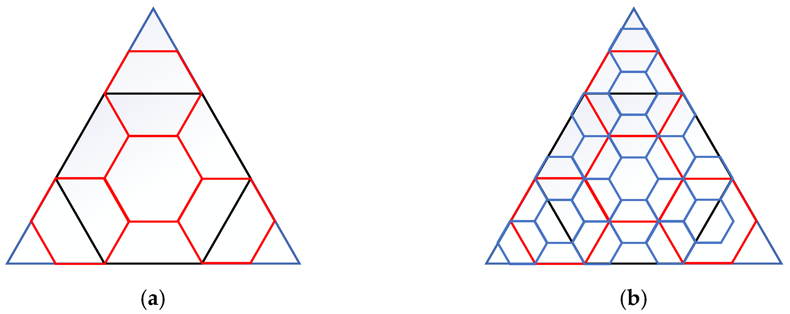
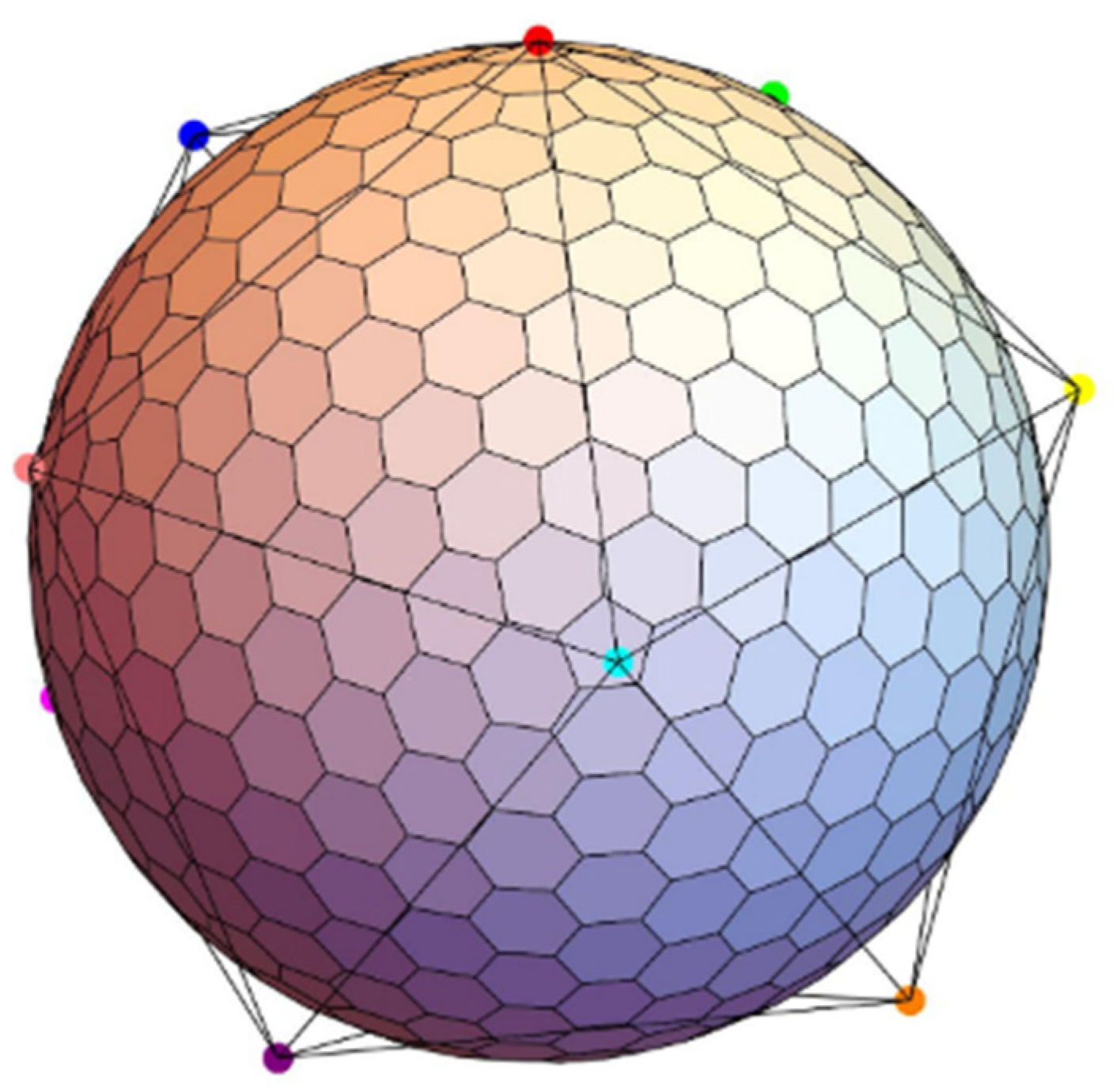
2.1. Construction of Icosahedral Hexagonal Discrete Grid System

The icosahedron is a regular polyhedron composed of twenty regular triangles, with a total of 30 edges and 12 vertices. It can be used to solve the problem of simplifying the division of the earth. The correspondence between the currently widely used regular icosahedron and the earth is as follows: the vertices of the icosahedron coincide with the poles of the earth, as shown in Figure 1a, and the expanded view of the regular icosahedron is shown in Figure 1b.

In order to construct a global discrete grid code, it is necessary to perform an initial segmentation based on a single triangular plane of the regular icosahedron and then refine the segmentation structure and achieve hierarchical segmentation. Aperture 4 hexagonal division is performed on each triangular surface. Grids at different levels are recursively generated using the above geometric structure, and the grid units on different levels of grids show a father–child inheritance relationship [3]. This paper will take one of the most commonly used subdivision structures, the Type I subdivision structure. The hierarchical subdivision structure on a single triangle in the Type I subdivision structure is shown in Figure 2. Hexagons with different colors represent different levels of grid division, in which black is the first layer, red is the second layer and blue is the third layer.

The generated results of plane hexagonal grid division can generate a spherical hexagonal grid tennis surface model by inverse ISEA projection. The lines formed by these spherical hexagonal boundaries divide the earth’s surface into equal-area spatial subdivision curves, and the spherical grid formed by the subdivision curves does not have the problem of bipolar oscillation, and the grid elements are evenly distributed on the global surface. Finally, it is projected on the spherical surface to form a hexagonal global discrete grid partition structure I of the icosahedron, as shown in Figure 3; all surfaces are covered by hexagons except for 12 vertices that are pentagons. Moreover, the grid on the sphere has the characteristics of infinite subdivision and can obtain any particle-scale grid through subdivision.

2.2. Vector Data Modeling Based on Icosahedral Hexagonal Grid

Vector data constitute an abstract representation model of spatial entities that abstracts spatial entities in the real world into targets with certain spatial relationships mainly in the form of points, lines, and polygons [22]. Studies have shown that in a general sense, the expression of raster data and vector data in the real world is consistent, because vector data are suitable for infinitely subdivided grids, and the size of the grid unit is the error range of the vector data [23]. However, this error range does not affect the spatial relationship inference of vector data. Using hexagonal discrete grids to reorganize and manage vector data is actually a process of gridding and reorganizing vector data.

2.2.1. Coordinate System of Hexagonal Grid

The hexagonal grid, due to its unique structural characteristics, differs from traditional Cartesian coordinate systems. Traditional geographic coordinate systems are based on orthogonal coordinate systems. Therefore, constructing a grid coordinate system based on the geometric structure and layout of the hexagonal grid is necessary. The establishment of the IJ coordinate system for hexagonal grids first requires determining the final geometric origin and orientation based on the layout pattern of the hexagonal grid. Subsequently, this paper establishes a coordinate system oriented at 120° based on the origin and a conversion model with the Cartesian coordinate system is developed accordingly. Figure 3 illustrates the IJ coordinate system, which originates from the coordinate origin and extends along the I and J axes in the original direction and at an angle of 120°, utilizing integer encoding for expansion. For data in any region, translation along the coordinate axes is required.

As shown in Figure 4, the conversion relationship between IJ and orthogonal coordinate system is established according to the following coordinate projection:

$$\mathrm{A}\left(\mathrm{x},\mathrm{y}\right)=\mathrm{A}\left(\mathrm{i},\mathrm{j}\right)·\left(\begin{array}{cc} 1& 0\\ -{\displaystyle \frac{1}{2}}& {\displaystyle \frac{\sqrt{3}}{2}}\end{array}\right)$$

(1)

The side length of the hexagonal grid cell is assumed to be 1, so Cartesian coordinates $\mathrm{A}\left(\mathrm{x},\mathrm{y}\right)$ and grid coordinates $\mathrm{A}\left(\mathrm{i},\mathrm{j}\right)$ can be effectively transformed into one another. This paper develops a bi-directional fast conversion algorithm for geographic coordinates and grid codes based on a hybrid strategy, facilitating the transformation of vector data into hexagonal grid data.

2.2.2. Determination of Gridding Levels

Studies have shown that, in a broad sense, raster data and vector data have consistent representations in the real world since vector data are suitable for infinitely fine grid subdivisions and the size of the grid cell corresponds to the error range of the vector data. However, this error range does not affect the spatial relationship reasoning of vector data. Vector terrain map data, for example, are very common in spatial vector data. According to the current Chinese topographic map framework standard, 8 national-series basic-scale topographic maps (1:5000, 1:200,000,000,000) and other non-basic-scale topographic maps have been authorized. These standard vector data usually include accuracy information. For example, for a vector data scale of 1:10,000, the map scale accuracy is approximately 10,000 × 0.0001 = 1 m, while for a vector data scale of 1:1,000,000, the map scale accuracy is 1,000,000 × 0.0001 = 100 m. This accuracy information exists in any spatial data, and vector data generated from standards must have accuracy assessment and explanation. For other vector data that truly lack accuracy information, the significant digits in the coordinates can provide some help. In addition, accuracy information of vector data can help find a suitable grid with a corresponding size.

Using the hexagonal Discrete Global Grid System (DGGS) of the ideal icosahedron as an example (with a subdivision pattern of the 4-hexagon aperture ISEA3H subdivision) and employing the Snyder equal-area projection as the DGGS projection model, which is widely used in the construction of hexagonal DGGSs,

Table 1. Aperture 4 hexagonal global discrete grid cell area attributes.

Res	Number of Cell *	Hexagonal Area (km2)	Pentagonal Area (km2)
1	32	17,002,187.39080	14,168,489.49230
2	122	4,250,546.84778	3,542,122.37308
3	482	1,062,636.71193	885,553.59327
4	1922	265,659.17798	221,382.64832
5	7682	66,414.79448	55,345.66208
6	30,722	16,603.69862	13,836.41552
7	122,882	4150.92466	3,459,903,883
8	491,522	1037.73116	864.77597
9	1,966,082	259.43280	216.19400
10	7,864,322	64.85821	54.04850
11	33,457,282	16.21455	13.51212
12	125,829,122	4.05364	3.37803
13	503,316,482	1.01341	0.84451
14	2,013,265,922	0.25335	0.21113
15	8,053,063,682	0.06334	0.05278
16	32,212,254,722	0.01584	0.01320

* Each layer of grid has a Pentagon at 12 vertices, and this column refers to the number of all grid units at each level.

records the area of grid cells on a discrete grid with subdivision level n with the radius of the earth being 6,371,007.22347 m. According to the structure shown in Figure 1, Figure 2 and Figure 3, Aperture 4 hexagonal global discrete grid cell area attributes are shown in Table 1.

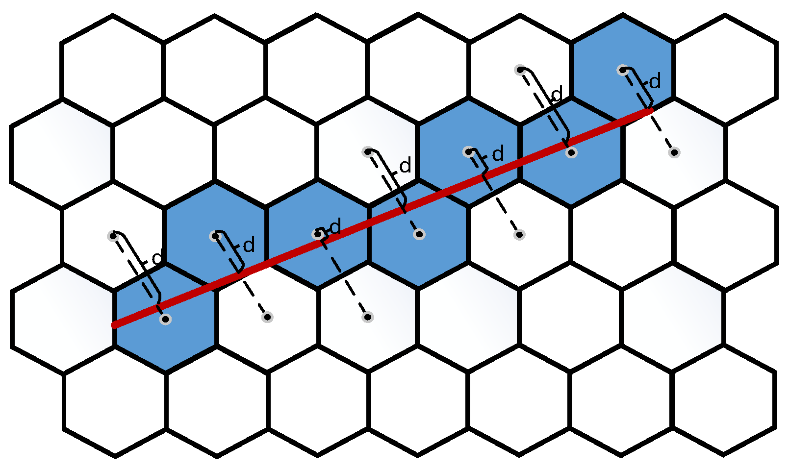
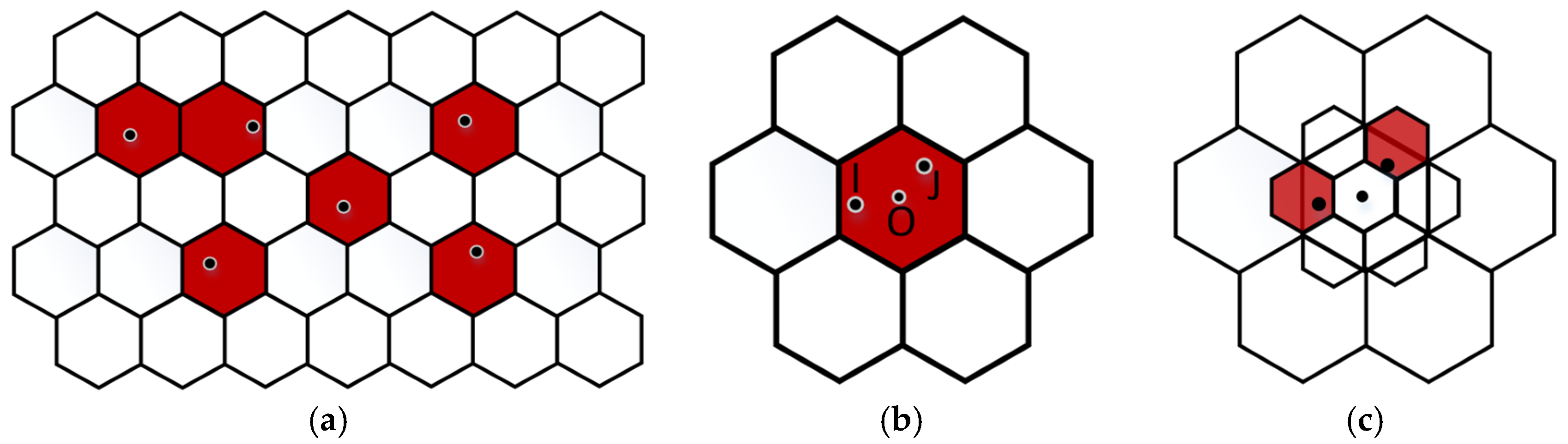
2.2.3. Gridding Method

For point data, the point-in-polygon method is commonly used to obtain grid cells of a specific scale for vector data. If a point falls within a particular grid cell, the cell is marked and the attribute value of the point is copied to the grid cell. The converted grid can be used to represent point data in a more organized and efficient way. It can also be used for various spatial analysis operations such as clustering and density analysis.

The Bresenham algorithm (Algorithm 1) based on the hexagonal grid structure is used to quickly generate straight line segments between each turning point. As shown in Figure 5, the Bresenham algorithm is a method for generating lines in computer graphics based on an error-discriminant formula.

Where the red line segment is the target linear vector data, and d is the distance from the calculated line segment to the center point of the neighboring grid, and the gridded unit is judged accordingly. The blue area is the grid unit corresponding to the vector data. Based on the IJ coordinate system, the calculation process of the Bresenham algorithm is as follows:

Algorithm 1. The Bresenham algorithm

//The coordinate system is rotated counterclockwise by 120 degrees to make the cases where the slope is less than or equal to 1 become horizontal   dx = x2 − x1   dy = y2 − y1   rx = round(dx * cos(2 * pi/3) − dy * sin(2 * pi/3))   //To obtain the difference in the rotated X-direction   ry = round(dx * sin(2 * pi/3) + dy * cos(2 * pi/3))   //To obtain the difference in the rotated Y-direction   //The Bresenham algorithm on the horizontal coordinate system is invoked   d = 0   y = y1   for x from x1 to x2:     yapprox = y + ry/rx     if d + abs(yapprox − y)<=0.5:       y = yapprox       d = d + abs(yapprox − y)     else:       d = d + abs(yapprox − y) − 1

For polygonal data, each edge of the polygon is traversed and the Bresenham algorithm is used to grid the edge and mark it on the grid. Based on the gridded boundary data, all edges of the polygon are traversed to find the points intersecting with the scan line. The scan line algorithm is then used to activate and fill the interior units of the polygon.

In this type of grid-based vector data record, there are three types of information: geometric information, attribute information, and topological information. Geometric information is the basic and fundamental spatial information of all vector information, consisting of point coordinates. The basic steps of data record are as follows: (1) replacing the coordinate points in geometric information with the encoding sequence of grid units, (2) preserving attribute information, and (3) preserving topological information. The vector data record mode on a discrete grid is equivalent to the traditional vector data record mode except in terms of coordinate recording. The difference mainly lies in the data expression; because the grid subdivides continuous space, the data expression must conform to the subdivision spatial principle.

2.3. Accuracy Evaluation of Gridded Vector Data

2.3.1. Error Sources and Classification of Vector Data Gridding

The process of vector data gridding is accompanied by information loss, just like the process of mapping, and errors are inevitable regardless of the transformation algorithm. In the gridding process of vector data, errors exist in parameters such as position, area, perimeter, shape features, topological structure features, and attributes, and these errors are influenced by parameters such as data sources, gridding algorithms, and data structure features [24]. Even if the input data are the same, different gridding methods may produce different results. Gridding of vector data is an important step in spatial analysis and modeling, and its accuracy directly affects the accuracy and credibility of subsequent analysis and model establishment. Higher accuracy in vector data gridding can ensure the accuracy of analysis results and spatial resolution of data, improve data processing efficiency and the visualization effect of analysis results, and provide more precise, reliable, and effective support for planning, decision making, and research [25]. Therefore, accuracy evaluation is also an important task in vector data gridding. More research is needed to improve the accuracy of gridding.

The sources of errors in vector-to-grid data conversion can be attributed to several factors. These include the following.

Resolution error: Vector data may contain details that cannot be accurately represented in grid data due to differences in resolution. This can result in a certain degree of resolution error.

Shape error: Vector data consist of lines and polygons while grid data are composed of pixels. The conversion process from vector to raster may cause changes in the shape of the original vector data, leading to shape error.

Topology error: Vector data describe spatial information based on topology relationships, while grid data describe spatial information based on pixel positions. The conversion process from vector to grid may result in changes to topology relationships, resulting in topology error.

Data accuracy error: Vector data may contain errors in data accuracy, such as in coordinate precision and topology precision, which can also be propagated and diffused during gridding, leading to a certain degree of error.

Encoding error: Vector data and grid data use different encoding methods, which may lead to encoding errors during the conversion process.

The precision of vector data forms the foundation of data recording and representation, and data with different precision are assigned to corresponding grid cells, resulting in grid data containing information on precision and scale. The recognized indicators for evaluating GIS spatial data quality include positional accuracy, attribute accuracy, completeness, logical consistency, semantic accuracy, temporal accuracy, and lineage. During the gridding process of different types of vector data, the data’s positions, geometric structures, and topological relationships undergo changes that vary with the data source, gridding algorithm, and data structure. Discretizing vector features into grid cells is the core problem of research on discrete global grid systems. For point features, grid processing is relatively simple, and grid cells corresponding to their scales can be used to represent them, while for line and polygon features, all grid cells covered by their scales must be determined. Although many research teams have proposed geometric preservation methods based on angle, length, and area, they have neglected to preserve topological relationships. Therefore, this paper proposes a universal system of precision evaluation indicators for the three types of vector data, as shown in Figure 6, to evaluate the similarity between gridded vector data and original vector data.

2.3.2. Accuracy Evaluation Metrics for Point Data

Point data, devoid of length and width, solely encapsulate geographical coordinates, attribute parameters, and topological relationships. Notably, attribute coordinates are directly assigned during transformation processes, eliminating the need for deviation assessment or judgment due to their inherent accuracy. Consequently, the uncertainty assessment of point data primarily focuses on geographical deviations and topological distortions. The evaluation of geographical deviations is predicated based on the Euclidean distance between the geographical coordinates of vector points and the centroid of the grid cell in which they reside post transformation. As the grid hierarchy deepens, leading to smaller grid cells, this deviation tends to diminish progressively.

Figure 7a illustrates the schematic of converting point-based vector data within a hexagonal grid system. The determination of the grid cell in which a point data falls, based on the extent of the grid cell at a specified hierarchy, allows for the calculation of the mean distance between the centroid coordinates of that grid cell and the coordinates of the vector point data. This calculation quantifies the geographical deviation of point data during the grid transformation process at that hierarchical level $\mathrm{D}={\displaystyle \frac{{{\displaystyle \sum }}_1^{\mathrm{n}}\sqrt{{\left({\mathrm{X}}_{\mathrm{i}}-{\mathrm{X}}_{\mathrm{oi}}\right)}^2+{\left({\mathrm{Y}}_{\mathrm{i}}-{\mathrm{Y}}_{\mathrm{oi}}\right)}^2}}{\mathrm{n}}}$.

The evaluation criteria for this type of point topological distortion are given thus: ${\mathrm{If} \mathrm{x}}_{\mathrm{i}}\ne {\mathrm{x}}_{\mathrm{j}}\left|\right|{\mathrm{y}}_{\mathrm{i}}\ne {\mathrm{y}}_{\mathrm{j}}{\displaystyle \cap }{\mathrm{code}}_{\mathrm{i}}={\mathrm{code}}_{\mathrm{j}}\to \mathrm{Intersects} \mathrm{Distortions}$. In the case of point features, if the spatial coordinates of two original points are identical, then the topological structures of these two point features are equal; otherwise, they are disjoint. After grid-based processing of point features, two original disjoint point features can be transformed into the same grid unit, and the topological relationship of point feature objects changes from disjoint to equal.

After conducting a topological distortion detection on the initial gridding results, all related point objects exhibiting topological distortions will have been identified. Subsequently, these topological distortions can be corrected. Given the multi-resolution hierarchical nature of the gridding system, the geometric precision of the point objects exhibiting topological distortions can be enhanced by describing their location information using a higher-level grid cell. If topological distortions persist, even at this increased resolution, the process is repeated using progressively higher-level grid cells until all topological distortions are eliminated, as shown in Figure 7b,c.

2.3.3. Accuracy Evaluation Metrics for Line Vector Data

A vector line is a one-dimensional geometric object represented by a set of vector points and composed of connected line segments. Each pair of consecutive points defines a line segment. The precision evaluation indicators for linear vector data consist of three levels, namely, geographic deviation, shape deviation, and topological distortion. Linear data, being a chained collection of a series of point data, necessitate a scientific approach to calculating geographical coordinate deviations that acknowledges their geometric characteristics. Neglecting these characteristics in the deviation calculations is unwarranted. Therefore, a representative parameter for geographical deviation can be derived by computing the mean square error (MSE) of the coordinate deviations at the midpoints of the lines connecting the start point to each turning point. This approach captures the inherent deviations along the linear feature, offering a more accurate assessment of the geographical deviations: ${\mathrm{D}}_{\mathrm{line}}=\sqrt{{\displaystyle \frac{{{\displaystyle \sum }}_1^{\mathrm{n}}{\mathrm{D}}_{\mathrm{i}}\left(\frac{{\mathrm{P}}_{0\mathrm{x}}+{\mathrm{P}}_{\mathrm{ix}}}{2},\frac{{\mathrm{P}}_{0\mathrm{y}}+{\mathrm{P}}_{\mathrm{iy}}}{2}\right)}{\mathrm{n}}}}$.

In comparison to point data, linear data, besides attributes, possess shape characteristics that cannot be transformed losslessly during conversion processes [26]. Linear geographical data typically embody two primary attributes: length and direction. These attributes serve as the basis for quantitatively evaluating the geometric distortions of linear vector data during transformation. Specifically, angular distortion can be calculated based on the angles formed between the multi-segment straight-line representation of the linear entity and the gridded data post conversion. Here, the distinction between clockwise and counterclockwise angles is not made, and the absolute value of the angular deviation is taken as the metric for assessment.

$${\mathsf{\theta }}_{\mathrm{dis}}={\displaystyle \frac{{{\displaystyle \sum }}_{\mathrm{i}=1}^{\mathrm{n}}\left|\Delta {\mathsf{\theta }}_{\mathrm{i}}\right|}{\mathrm{n}}}$$

(2)

Here, $\Delta {\mathsf{\theta }}_{\mathrm{i}}$ denotes the angular deviation of the i-th line segment, with a total of n line segments comprising the entire linear entity. To achieve a standardized assessment, the cosine of the mean angular deviation is computed as $S_{dir}=cos{\mathsf{\theta }}_{\mathrm{dis}}$, with a result closer to 1 indicating smaller angular deviation.

The length distortion of linear data is determined by the mean of the length ratios before and after the conversion of its segments. Let L represent the side length of the hexagonal grid cell at a specific hierarchy. The overall length distortion of linear data is calculated using Equation (5), where ${\mathrm{L}}_{\mathrm{distortion}}$ closer to 1 signifies lesser length distortion during the conversion process:

$${\mathrm{L}}_{\mathrm{distortion}}={\displaystyle \frac{{{\displaystyle \sum }}_{\mathrm{i}=1}^{\mathrm{n}}\frac{\sqrt{3}\mathrm{Ln}}{{\mathrm{L}}_{\mathrm{vector}}}}{\mathrm{n}}}$$

(3)

Here, ${\mathrm{L}}_{\mathrm{vector}}$ is the length of the vector segment.

According to the 9-intersection model, there are two topological relationships for linear entities: disjoint and intersect. However, in the process of gridization, there exist distortions of topological relationships due to the precision limitation of grid units, including the following types.

A.

Disjoint becomes overlap

As shown in Figure 8, because the two linear entities are too close, they are judged as overlapping in the process of gridization and become the same linear entity. The detection method is such that the original vector linear data are disjoint, but ${\mathrm{codeSet}}_{\mathrm{i}}{\displaystyle \cap }{\mathrm{codeSet}}_{\mathrm{j}}\ne \varnothing$.

B.

Open line entity becomes closed line entity

As shown in Figure 9, the fact that the distance between the two endpoints of the line entity is smaller than the internal distance of the gridded cell leads to the result that the line entity becomes a closed line entity because it is judged as a gridded cell during the gridding process. This distortion is detected by the line entity ${\mathrm{linepoint}}_{1,2,\dots \mathrm{n}}$ after gridding ${\mathrm{codeSet}}_1={\mathrm{codeSet}}_{\mathrm{n}}$.

2.3.4. Accuracy Evaluation for Polygon Data

The accuracy evaluation for the polygon data also includes three levels, which are geographic deviation, geometric features, and topological features.

(1)

Geographical deviation of polygon vector data

Areal data are essentially collections of single or multiple closed linear vector data, comprising multiple arcs [21]. Consequently, the quantitative assessment of polygon data can be performed based on the median of the geographical deviations derived from the linear data that constitute its arcs: ${\mathrm{D}}_{\mathrm{polygon}}=\sqrt{{\displaystyle \frac{{{\displaystyle \sum }}_1^{\mathrm{n}}{\mathrm{D}}_{\mathrm{line}}^{\mathrm{i}}}{\mathrm{n}}}}$.

(2)

Geometric features of polygon vector data

The geometric features of facet vector data are mainly shapes.

Specifically, the geometric characteristics of the surface vector data can be evaluated quantitatively in terms of distance similarity, direction similarity, and shape similarity.

Distance similarity: The centroid of planar vector data is usually used to identify and annotate the center of an area. It is also often used as a reference point in spatial analysis to calculate the distance between polygons and provide a reference for spatial clustering analysis. As the center point of planar vector data, the centroid can effectively simplify and enhance various spatial analysis and visualization tasks in geographic information systems. For a polygon determined by a label point, the calculation formula for its centroid $(C_X,C_Y)$ is as follows:

$$C_X={\displaystyle \frac{1}{6A}}{\displaystyle \sum }_{i=1}^n\left(x_i+x_{i+1}\right)\left(x_i{y}_{i+1}-x_{i+1}{y}_i\right)$$

(4)

$$C_Y={\displaystyle \frac{1}{6A}}{\displaystyle \sum }_{i=1}^n\left(y_i+y_{i+1}\right)\left(x_i{y}_{i+1}-x_{i+1}{y}_i\right)$$

(5)

Here, $(x_i,y_i)$ are the coordinates of each vertex of the polygon, and $A$ is the area of the polygon, which can be calculated by dividing the polygon into multiple triangles. The calculation formula is as follows:

$$A={\displaystyle \frac{1}{2}}{\displaystyle \sum }_{i=1}^n\left(x_i{y}_{i+1}-\left(x_{i+1}{y}_i\right)\right)$$

(6)

Here, the values of the $i=1$ subscripts need to be calculated in a cyclic order.

Directional similarity: During the conversion process, the shape and orientation of the polygon may be offset, and the direction of the surface data can be determined based on the diagonal line. Therefore, the average angle of multiple diagonal lines before and after the polygon conversion can be calculated to determine the direction similarity:

$${\mathrm{S}}_{\mathrm{dir}}={\displaystyle \frac{{{\displaystyle \sum }}_0^{\mathrm{n}}\mathrm{i},\mathrm{jcos}(|\mathrm{Arctan}(\frac{{\mathrm{y}}_{\mathrm{j}}-{\mathrm{y}}_{\mathrm{i}}}{{\mathrm{x}}_{\mathrm{j}}-{\mathrm{x}}_{\mathrm{i}}})-\mathrm{Arctan}(\frac{{\mathrm{y}}_{\mathrm{j}}^{\prime }-{\mathrm{y}}_{\mathrm{i}}^{\prime }}{{\mathrm{x}}_{\mathrm{j}}^{\prime }-{\mathrm{x}}_{\mathrm{i}}^{\prime }})|)}{\mathrm{n}}}$$

Shape similarity: For polygon data, measurement parameters such as area and perimeter are crucial. After gridding, the area of surface data changes from a continuous value to discrete data with the area of the grid unit as the unit. In order to judge the changes in these parameters before and after the conversion, shape similarity is mainly based on area ratio (AR), overlap area ratio (OAR), perimeter ratio (PR), minimum external circle (MEC) area ratio, and minimum external rectangle (MBR) area ratio. The error-based similarity of one of these features’ metrics V (area, perimeter, etc.) is calculated as follows:

$${\mathrm{S}}_{\mathrm{V}}\left(\mathrm{A},\mathrm{B}\right)=1-{\displaystyle \frac{\left|{\mathrm{V}}_{\mathrm{A}}-{\mathrm{V}}_{\mathrm{B}}\right|}{\max \left({\mathrm{V}}_{\mathrm{A}},{\mathrm{V}}_{\mathrm{B}}\right)}}$$

(7)

Here, ${\mathrm{S}}_{\mathrm{V}}\left(\mathrm{A},\mathrm{B}\right)$ is the similarity of the area (perimeter) metric V, ${\mathrm{V}}_{\mathrm{A}}$ is the value of the V metric of the vector data, and ${\mathrm{V}}_{\mathrm{B}}$ is the value of the V metric of the gridded image B. This calculation of similarity indicators normalizes all indicators to 1, i.e., the closer the indicator calculation result is to 1, the higher the accuracy of this parameter is.

The shape similarity of the facet vector data contains multiple indicators, and in order to make a comprehensive evaluation of the results of multiple indicators, the weights of the above five accuracy evaluation indicators (the shape similarity is mainly based on the area ratio (AR), the overlap area ratio (OAR), the perimeter ratio (PR), the minimum externally connected circle (MEC) area ratio, and the minimum externally connected rectangle (MBR) area ratio) are determined using the Analytic Hierarchy Process (AHP).

Layer 1: Target layer. The objective of this model is to evaluate the information retention and similarity of the hexagonal grid image to the original image before and after conversion. Therefore, the similarity is considered as a predefined objective for decision making.

Layer 2: Indicator layer. Through literature research, five metrics, namely area ratio, overlapping area ratio, perimeter ratio, minimum external circle (MEC) area ratio, and minimum area external rectangle (MBR) area ratio, are selected as quantitative metrics to quantify the information retention, similarity to the original image, and structural similarity before and after image conversion. These five metrics are intermediate evaluation criteria.

Layer 3: Procedural layer. The objects we analyze are the original remote sensing image and the sampled remote sensing image based on hexagonal grid, so the basic decision plan can be divided into the original remote sensing image and the hexagonal grid image.

Based on the above problem analysis, we establish the hierarchical analysis model of the original remote sensing image and the hexagonal grid image.

Then, we use the hierarchical analysis method to determine the weights of the evaluation factors.

A.

Construction of judgment matrix

For each pair of criteria, we assign a relative importance score between 1 and 9, where 1 means the criteria are equally important and 9 means the criteria are much more important. We create a pairwise comparison matrix: A = (${\mathrm{a}}_{\mathrm{ij}}$)

$${\mathrm{a}}_{\mathrm{ik}}\times {\mathrm{a}}_{\mathrm{kj}}={\mathrm{a}}_{\mathrm{ij}}$$

(8)

Here, ${\mathrm{a}}_{\mathrm{ij}}$ is set by criteria 1~9.

After analyzing the impacts of the five major indicators on the total target, the following determination matrix A is constructed, and we normalize the pairwise comparison matrix by dividing each element in each row by the row sum. This gives us a matrix B of relative weights for each criterion.

$$\mathrm{A}=\left(\begin{array}{cc}\begin{array}{cc}1& 3\\ {\displaystyle \frac{1}{3}}& 1\end{array}& \begin{array}{ccc}5& 6& 4\\ 3& 5& 3\end{array}\\ \begin{array}{cc}{\displaystyle \frac{1}{5}}& {\displaystyle \frac{1}{3}}\\ {\displaystyle \frac{1}{6}}& {\displaystyle \frac{1}{5}}\\ {\displaystyle \frac{1}{4}}& {\displaystyle \frac{1}{3}}\end{array}& \begin{array}{ccc}1& 3& 2\\ {\displaystyle \frac{1}{3}}& 2& 3\\ {\displaystyle \frac{1}{2}}& {\displaystyle \frac{1}{3}}& 1\end{array}\end{array}\right)\mathrm{B}=\left(\begin{array}{cc}\begin{array}{ccc}0.1429& 0.4286& 0.7143\\ 0.0833& 0.2500& 0.7500\\ 0.0882& 0.2647& 0.7941\end{array}& \begin{array}{cc}0.8571& 0.5714\\ 1.2500& 0.7500\\ 1.7647& 1.1765\end{array}\\ \begin{array}{ccc}0.0895& 0.2237& 0.3368\\ 0.0947& 0.2842& 0.4737\end{array}& \begin{array}{cc}1.0000& 2.3684\\ 0.8947& 1.0000\end{array}\end{array}\right)$$

(9)

B.

Determine the weight

We calculate the weighted score (

Table 2. Weights of the five evaluation indicators.

Weights of the Five Evaluation Indicators
k	AR	OAR	PR	MEC	MBR
W	0.7143	0.2500	0.7941	0.4474	0.3789

) for each criterion by multiplying the normalized weight by the degree of importance assigned to that criterion.

Thus, the geometric features of the polygon vector data are combined with the following index:

$$\mathrm{G}={\displaystyle \frac{0.7143\times \mathrm{AR}+0.25\times \mathrm{OAR}+0.7941\times \mathrm{PR}+0.4474\times \mathrm{MEC}+0.3789\times \mathrm{MBR}}{2.5847}}$$

(10)

It is worth noting that the indicators and their impact factors can be modified depending on the direction and focus of the application to the grid vector data.

(3)

Attribute accuracy loss assessment method

Polygon data usually have attribute information, The attribute accuracy can be quantitatively evaluated according to the change in land area. The basic idea of this method is as follows: we count the area Av of each land class in the land cover vector data and use it as the base area, count the area A of each land class under different grid sizes, and compare the grid area of each land class with its corresponding base area so as to obtain the relative area accuracy loss of each land class under different scales. The calculation formula is as follows:

$$E_i={\displaystyle \frac{(A_g^i-A_v^i)}{A_v^i}}\times 100\%$$

(11)

Here, $i$ is the land class code, $A_g^i$ is the area of the land class based on the grid organization, $A_v^i$ is the area of the land class calculated using vector data, and $E_i$ is the area precision loss of the $i$ land class.

The average area precision loss of the entire study area can be obtained by the weighted average of the relative area precision losses of each land class, with the weight being the percentage of each land class in the entire study area. The formula is as follows:

$$\mathrm{E}={\displaystyle \sum }_1^{\mathrm{i}}(E_i\times {\displaystyle \frac{A_v^i}{A}})\#\left(11\right)$$

Here, $\mathrm{E}$ is the average area precision loss (%) of the entire study area and A is the total area of the study area.

(4)

Topological feature metrics for polygon vector data

The topological similarity metric of polygon data is based on the 4-intersection model proposed by Egenhofer et al. and the topological relationship defined by the 9-intersection model [27], which is based on the 4-intersection model. The 9-intersection model classifies spatial relations by comparing the intersection of the interiors, boundaries, and exteriors of 2 entities as empty or non-empty. This model identifies 8 face-to-face relations (separated, connected, overlapping, equal, covered, covered, contained, and contained). This topological relationship is defined as a conceptual distance value, and the distance metric is performed through the topological relationship between graphs to obtain the topological relationship similarity metric.

While the topological relationship of face objects is relatively complex, the polygons do not overlap with each other in various vector datasets that are currently common. Then based on the nine-intersection model, there are only two topological relationships between different face objects, meet (Meet, F***T****) and disjoint (Disjoint, FF*FF****). But in the process of hexagonal gridding, two vector faces may turn from originally connected to disjoint, and the individual facet data may be split or disappear in this case.

Specifically, Figure 10 includes the following four cases of topological distortion.

In Figure 9a, according to the principle of area dominance, the relatively small polygon data B may disappear directly after gridding. In Figure 9b, some polygon data connected by narrow areas may have their connection areas divided into other facets during gridding, which also results in the originally connected polygon data being split into two blocks of A and C. In Figure 10c, also due to the narrow connection areas, the originally connected B, and in Figure 10d, the topology of A enclosing B, become connected after gridding because the enclosing area is too narrow. All these topological eventualities occur because the area of the polygon data or topologically sensitive regions is too small to be expressed in an area-dominated structure. This is because when adaptively increasing the grid level, the focus should be on unstable lattice elements that intersect multiple vector faces because these lattice elements may be attributed to other lattice elements that intersect with them. According to the nine-intersection model, the topological relations of these unstable lattice elements are $R_9\left(Ploygon,VariableCell\right)=\left(TTTT\ast T\ast \ast T\right)$.

3. Experimental Results and Analysis

3.1. Point Data Conversion and Uncertainty Assessment

The point data are used to determine the hexagonal grid cells where the points are located using the drop point method, and the level of the converted grid is the 14th level, marked by the coordinates of the center point of the grid cells, as shown in Figure 11.

Among them, for the point data, the coordinate difference before and after conversion is calculated in 872 subway coordinate points in Beijing, and the average value is 0.096° (8.624 km). Among 872 points, a total of 12 points have point topological distortion, and this distortion can be avoided in the 15th layer grid, as shown in Figure 12.

The red area is the case of geometric distortion of point data. The enlarged image in the upper left corner of Figure 12 shows that most of the topological distortions (equal phase separation and transformation) of point data appearing in the 14th layer grid have been resolved in the 15th layer grid, For example, two points were originally divided into the same grid unit in the 14th layer grid while after the re-division of the high-level grid, they were divided into two different grid units. However, there are still cases where some points that are too close are still divided into one unit, which can also be solved by increasing the grid level. It should be noted that for point data, the grid level that can solve topological distortion should be thus: the side length of the grid unit of this level is L, and the shortest distance of point data is greater than $\surd 3\mathrm{L}$.

3.2. Transformation and Uncertainty Assessment of Line Data

The linear data of G45 and the Daguang Expressway in Beijing, China were selected as the test data to carry out an experiment, and the Bresenham algorithm was used to realize the transformation and storage of grid data on the 10th, 11th, 12th, and 13th floors. The results are shown in Figure 13.

For the data of this section of highway, the quantitative evaluation index system was used, and the results are shown in

Table 3. Accuracy evaluation results of line data.

Grid Level	Geographical Deviation (KM)	Angular Distortion	Length Distortion
10	12.67	5.1374	1.0843726
11	3.54	2.0845	0.9341268
12	1.29	1.0547	1.5147326
13	0.76	0.4731	0.9718905

.

It can be seen that with an increase in the grid level, the accuracy level of each index was also increasing. In actual use, the data of the corresponding level can be selected for organization and management according to the accuracy requirements.

3.3. Transformation of Polygon Data and Uncertainty Assessment

The polygon data were selected from the administrative boundary data of Beijing, and the gridding of the polygon vector data was realized by using the filling algorithm, and the transformation levels were the 10th, 11th, and 12th layers, as shown in Figure 14.

The geographic deviation was calculated for three levels, 26.6 km for level 10, 17.4 km for level 11, and 11.3 km for level 12. For the geometric characteristics of the polygon data, the area in the vector data range of Beijing was 16,373,770,236.4 m², and the evaluation indexes of the accuracy of the geometric characteristics of the grid at different levels were calculated, and the comprehensive evaluation indexes were calculated. The evaluation results for the geometric accuracy of polygon data are shown in

Table 4. Evaluation results of geometric accuracy of polygon data.

Grid Level	Number of Grid Cells	Area Ratio	Overlap Area Ratio	Perimeter Ratio	MEC Area Ratio	MBR Area Ratio	Composite Index
10	405	0.9297	0.9346	1.0615	0.9431	0.9513	0.9647
11	1489	0.9453	0.9578	1.0432	0.9678	0.9647	1.0435
12	5662	1.0212	0.9741	1.0225	0.9791	0.9815	1.0135

.

The accuracy of geographic deviation and geometric features of the polygon vector data significantly improved with an increase in the grid level. The accuracy of vector data gridding can be improved by gridding with higher levels of grids.

4. Conclusions

Based on the feature that the hierarchy of hexagonal grids can be divided infinitely, grids can be used to store unstructured emerging spatial big data including points, lines, human activities, etc. Hexagonal grids and vector data are two different forms of data management and data storage, with significant differences in data organization and expression. The precision of vector data is the basis of data records and data expressions, and grids of different expression sizes are used to illustrate different data of different precision levels. The data of different precision levels fall into the corresponding grid cells so that the grid data itself contain precision and scale information. This paper aimed to evaluate the accuracy of hexagonal-grid-based image data by establishing a suitable accuracy evaluation index system based on three levels—geographic deviation, geometric structural features, and topological distortion—and has provided a generalizable accuracy evaluation index system and evaluation method for hexagonal-grid-based vector data, which provides support for the further use of hexagonal-grid-based data. These generalized accuracy evaluation indexes can achieve better metrics, but there are problems such as artificially specified index weights or threshold determination, so in specific practice, appropriate feature indexes and similarity calculation methods need to be selected for specific application scenarios to improve the accuracy of similarity metrics. Hexagonal grids have significant potential for storing and analyzing complex spatial data, and future research could focus on developing more precise and accurate evaluation index systems, exploring new applications for hexagonal-grid-based data, and investigating integration with other data management and storage systems.

References

1. Sahr, K. Central place indexing: Hierarchical linear indexing systems for mixed-aperture hexagonal discrete global grid systems. Cartogr. Int. J. Geogr. Inf. Geovis. 2019, 54, 16–29. [Google Scholar] [CrossRef]
2. Yao, X.; Yu, G.; Li, G.; Yan, S.; Zhao, L.; Zhu, D. HexTile: A Hexagonal DGGS-Based Map Tile Algorithm for Visualizing Big Remote Sensing Data in Spark. ISPRS Int. J. Geo-Inf. 2023, 12, 89. [Google Scholar] [CrossRef]
3. Zhao, L.; Li, G.; Yao, X.; Ma, Y.; Cao, Q. An optimized hexagonal quadtree encoding and operation scheme for icosahedral hexagonal discrete global grid systems. Int. J. Digit. Earth 2022, 15, 975–1000. [Google Scholar] [CrossRef]
4. Nelson, R.C.; Samet, H. A consistent hierarchical representation for vector data. In Proceedings of the 13th Annual Conference on Computer Graphics and Interactive Techniques, Dallas, TX, USA, 31 August 1986; Volume 20, pp. 197–206. [Google Scholar]
5. Wang, L.; Ai, T.; Shen, Y.; Li, J. The isotropic organization of DEM structure and extraction of valley lines using hexagonal grid. Trans. Gis 2020, 24, 483–507. [Google Scholar] [CrossRef]
6. Amiri, A.M.; Samavati, F.; Peterson, P. Categorization and conversions for indexing methods of discrete global grid systems. ISPRS Int. J. Geo-Inf. 2015, 4, 320–336. [Google Scholar] [CrossRef]
7. Sahr, K.; White, D.; Kimerling, A.J. Geodesic Discrete Global Grid Systems. American Cartographer. Cartogr. Geogr. Inf. Sci. 2003, 30, 121–134. [Google Scholar] [CrossRef]
8. Mahdavi Amiri, A.; Alderson, T.; Samavati, F. Geospatial Data Organization Methods with Emphasis on Aperture-3 Hexagonal Discrete Global Grid Systems. Cartogr. Int. J. Geogr. Inf. Geovis. 2019, 54, 30–50. [Google Scholar] [CrossRef]
9. Gibb, R.G. The rHEALPix discrete global grid system. IOP Conf. Ser. Earth Environ. Sci. 2016, 34, 012012. [Google Scholar] [CrossRef]
10. Goodchild, M.F. The Application of Advanced Information Technology in Assessing Environmental Impacts. Soil Sci. Soc. Am. 1996, 48, 1–17. [Google Scholar]
11. Li, D.; Zhang, G.; Jiang, Y.H.; Shen, X.; Liu, W. Opportunities and challenges of geo-spatial information science from the perspective of big data. Big Data Res. 2022, 8, 3–14. [Google Scholar]
12. Zhao, L.; Li, G.; Yao, X.; Ma, Y. Code Operation Scheme for the Icosahedral Hexagonal Discrete Global Grid System. Geo-Inf. Sci. 2023, 25, 239–251. [Google Scholar]
13. Lunetta, R.; Congalton, R.; Fenstermaker, L.; Jensen, J.; Mcgwire, K.; Tinney, L.R. Remote sensing and geographic information system data integration: Error sources and Research Issues. Photogramm. Eng. Remote Sens. 1991, 57, 677–687. [Google Scholar]
14. Dutton, G. Universal geospatial data exchange via global hierarchical coordinates. In Proceedings of the International Conference on Discrete Global Grids, Santa Barbara, CA, USA, 26–28 March 2000. [Google Scholar]
15. White, D.; Kimerling, A.J.; Sahr, K.; Song, L. Comparing area and shape distortion on polyhedral-based recursive partitions of the sphere. Int. J. Geogr. Inf. Syst. 1998, 12, 805–827. [Google Scholar] [CrossRef]
16. Shortridge, A.M. Geometric variability of raster cell class assignment. Int. J. Geogr. Inf. Sci. 2004, 18, 539–558. [Google Scholar] [CrossRef]
17. Frolov, Y.S.; Maling, D.H. The accuracy of area measurement by point counting techniques. Cartogr. J. 1969, 6, 21–35. [Google Scholar] [CrossRef]
18. Congalton, R.G.; Green, K. Assessing the Accuracy of Remotely Sensed Data: Principles and Practices; CRC Press: Boca Raton, FL, USA, 2019. [Google Scholar]
19. Burrough, P.A.; McDonnell, R.A.; Lloyd, C.D. Principles of Geographical Information Systems; Oxford University Press: Oxford, UK, 2015. [Google Scholar]
20. Ma, Y.; Li, G.; Yao, X.; Cao, Q.; Zhang, L. A Precision Evaluation Index System for Remote Sensing Data Sampling Based on Hexagonal Discrete Grids. Int. J. Geo-Inf. 2021, 10, 194. [Google Scholar] [CrossRef]
21. Ma, Y.; Li, G.; Zhao, L.; Yao, X. An Accuracy Evaluation Method for Multi-source Data Based on Hexagonal Global Discrete Grids. In Proceedings of the International Conference on Spatial Data and Intelligence, Nanchang, China, 25–27 April 2024. [Google Scholar]
22. Li, Q.; Wang, T.; Zhu, J.; Zhang, F. Vector data rasterization based on rendering and pickup. Geomat. Inf. Sci. Wuhan Univ. 2010, 35, 917–919. [Google Scholar]
23. Wang, Y.; Chen, Z.; Cheng, L.; Li, M.; Wang, J. Parallel scanline algorithm for rapid rasterization of vector geographic data. Comput. Geosci. 2013, 59, 31–40. [Google Scholar] [CrossRef]
24. Vauglin, F. A practical study on precision and resolution in vector geographical databases. In Spatial Data Quality; Taylor & Francis: London, UK, 2002; pp. 127–139. [Google Scholar]
25. Van Der Knaap, W.G.M. The vector to raster conversion: (mis)use in geographical information systems. Int. J. Geogr. Inf. Syst. 1992, 6, 159–170. [Google Scholar] [CrossRef]
26. Zhou, J.; Ben, J.; Wang, R.; Zheng, M.; Yao, X.; Du, L. A novel method of determining the optimal polyhedral orientation for discrete global grid systems applicable to regional-scale areas of interest. Int. J. Digit. Earth 2020, 13, 1553–1569. [Google Scholar] [CrossRef]
27. Egenhofer, M.J.; Herring, J.J.T. Categorizing binary topological relations between regions, lines, and points in geographic databases. The 1990, 9, 76. [Google Scholar]
Figure 1. Model of icosahedron DGGS. (a) The relationship between icosahedron and spherical surface. (b) Diagram of the unfolded icosahedron surface.
Ijgi 14 00005 g001
Figure 2. Subdivision structure diagram of the Aperture 4 hexagon on the triangular surface. (a) Schematic diagram of the grid subdivided into the second layer (b) Schematic diagram of the grid subdivided into the third layer.
Ijgi 14 00005 g002
Figure 3. The third level spherical structure of the icosahedral hexagonal global discrete grid.
Ijgi 14 00005 g003
Figure 4. Schematic diagram of IJ coordinate system. (A) Schematic diagram of IJ coordinate system. (B) Conversion relationship between IJ and orthogonal coordinates.
Ijgi 14 00005 g004
Figure 5. Gridding process of linear data based on Bresenham algorithm.
Ijgi 14 00005 g005
Figure 6. Accuracy evaluation process of gridded vector data.
Ijgi 14 00005 g006
Figure 7. Illustration of grid-based transformation and topological distortion for point vector data. (a) Marked grid points for point vector data. (b) Topological distortion of point vector data. (c) Topological distortion of point data resolved by increasing LEVEL.
Ijgi 14 00005 g007
Figure 8. (a) Topological distortion of line entities, where phase separation becomes overlapping; (b) raising the grid level maintains the topological characteristics of the data.
Ijgi 14 00005 g008
Figure 9. (a) Topological distortion of line entities from open line entities into closed line entities; (b) raising the grid level to maintain the topological characteristics of the data.
Ijgi 14 00005 g009
Figure 10. Types of topological distortion of polygon vector data lattice meshing: (a) vector polygon lattice meshing faces disappear; (b) vector polygon lattice meshing is followed by splitting; (c) vector polygon lattice meshing becomes adjacent to each other or adjacent to each other; (d) vector polygon lattice meshing loses the enclosing topological relationship.
Ijgi 14 00005 g010
Figure 11. Conversion of point data.
Ijgi 14 00005 g011
Figure 12. Repairing point topological distortion by 15th grid.
Ijgi 14 00005 g012
Figure 13. Vector data gridding of Beijing Metro Line 13.
Ijgi 14 00005 g013
Figure 14. Gridding of Beijing administrative boundary surface vector data: (a) the 10th-level gridding of Beijing administrative district; (b) the 11th-level gridding of Beijing administrative district; (c) the 12th-level gridding of Beijing administrative district; (d) the geometric structure of the adjacent three levels of gridding.
Ijgi 14 00005 g014