Abstract
This study introduces an innovative scheme for classifying uncrewed aerial vehicle (UAV)-derived vehicle trajectory behaviors by employing machine learning (ML) techniques to transform original trajectories into various sequences: space–time, speed–time, and azimuth–time. These transformed sequences were subjected to normalization for uniform data analysis, facilitating the classification of trajectories into six distinct categories through the application of three ML classifiers: random forest, time series forest (TSF), and canonical time series characteristics. Testing was performed across three different intersections to reveal an accuracy exceeding 90%, underlining the superior performance of integrating azimuth–time and speed–time sequences over conventional space–time sequences for analyzing trajectory behaviors. This research highlights the TSF classifier’s robustness when incorporating speed data, demonstrating its efficiency in feature extraction and reliability in intricate trajectory pattern handling. This study’s results indicate that integrating direction and speed information significantly enhances predictive accuracy and model robustness. This comprehensive approach, which leverages UAV-derived trajectories and advanced ML techniques, represents a significant step forward in understanding vehicle trajectory behaviors, aligning with the goals of enhancing traffic control and management strategies for better urban mobility.
1. Introduction
1.1. Motivation
Traffic trajectory is crucial for traffic analysis, as it can reveal the movement patterns of vehicles within a transportation system. Understanding how traffic flows through intersections is essential to optimize efficiency, identify congestion points, and enhance overall safety. Many studies have developed different approaches to improve localization [1], positioning [2], attitude estimation [3], and control system security [4]. Therefore, advanced UAVs that provide accurate geolocation enable reliable monitoring and promote their application in traffic surveillance. The images captured using uncrewed aerial vehicles (UAVs) offer a comprehensive view of intersections; this facilitates the observation of various parameters and enables the extraction of each vehicle’s trajectory within the intersection. The extracted trajectory can be used to calculate traffic parameters, such as speed and acceleration, and provide a comprehensive representation of the movement and behavior of the tracked vehicles over time. Trajectory analysis plays a key role in building an intelligent traffic system and is particularly important for facilitating data-driven decision making. Therefore, this study utilized UAV-derived trajectories for analyzing trajectories at intersections.
1.2. Related Works
Various methods are employed to acquire traffic parameters, including inductive loop sensors embedded in road surfaces, closed-circuit television (CCTV), airborne optical remote sensing sensors, and UAVs for determining traffic flow. For example, Li [5] employed a dynamic linear model to integrate data from both inductive loop detectors and automatic number plate recognition systems. The loop detectors can be integrated with GPS-equipped probe vehicles for estimating urban traffic. Kong et al. [6] introduced an information fusion approach for urban traffic state estimation. The authors combined data from underground loop detectors and GPS-equipped probe vehicles. Additionally, CCTV camera images can be utilized to capture real-time traffic conditions. They provide essential data on vehicle counts, speeds, and congestion levels for effective traffic management and planning. Kurniawan et al. [7] developed an intelligent traffic congestion detection method with a convolutional neural network (CNN) and CCTV camera image feeds. The results showed that the CNN model that was trained on small grayscale CCTV images achieved 89.5% accuracy in detecting traffic congestion. Not only the ground-based system but also high-resolution aerial and space-borne images can be used to count vehicles. Guo et al. [8] introduced a vehicle counting method based on density maps that is specifically designed for remote sensing imagery with limited resolution. They utilized the enhanced CSRNet to demonstrate its effectiveness in counting vehicles from 1 m satellite images.
Traditional traffic flow monitoring systems, such as inductive loop sensors and CCTV, face limitations when monitoring specific locations. The installation and maintenance of inductive loop sensors may cause traffic disruptions and decrease pavement life, with the infrastructure being susceptible to damage from the activities of heavy vehicles. They may also be damaged during road maintenance. CCTV cameras also have inherent limitations, including a restricted angle and field of view, fixed position, and the potential for causing traffic disruptions during repairs; in contrast, UAVs offer significant advantages by providing complete coverage of intersections. This wide coverage enables a more comprehensive trajectory analysis, enabling the extraction of each vehicle’s trajectory at intersections. UAV-captured videos have proven to be more suitable for traffic monitoring tasks due to the low cost, high flexibility, and wider field of view offered by UAVs [9,10,11,12].
Machine learning (ML) and deep learning (DL) technologies have garnered significant attention for trajectory tracking. For example, Xu et al. [13] explored machine learning-based traffic flow prediction and intelligent traffic management, demonstrating that advanced ML algorithms can significantly enhance traffic flow prediction accuracy and enable proactive traffic management. Ke et al. [14] utilized a methodology involving the training of Haar cascade and a CNN for vehicle detection. Subsequently, they applied Kanade–Lucas–Tomasi (KLT) optical flow to extract motion vectors and introduced a novel supervised learning algorithm to estimate the traffic flow parameters. Biswas et al. [15] implemented a speed detection system for ground objects from aerial view images. They employed Faster R-CNN for object detection, a channel and spatial reliability tracker for tracking, feature-based image alignment for object location, and the structural similarity index measure to check the similarity between frames. Ke et al. [16] proposed a comprehensive unsupervised learning traffic analysis system using UAV videos. This system features a multiple-vehicle tracking algorithm and a traffic lane information extraction method. The tracking algorithm employs an ensemble vehicle detector and a KLT optical flow tracker. Additionally, the lane information extraction method involves modified Canny edge detection, adaptive DBSCAN for line clustering, lane boundary tracking in Hough space, and lane length calculation. Previous studies have indicated that DL technology can prove beneficial in deriving traffic parameters.
The results of trajectory tracking can be visualized and analyzed through a scatter plot or a space–time diagram. A scatter plot indicates the distribution of vehicles while a space–time diagram indicates the relationship between space and time for vehicles. Traffic parameters such as velocity and acceleration can be obtained from a vehicle’s trajectory. The space–time diagram is widely used to interpret and visualize tracked trajectories. For example, Khan et al. [17] unveiled diverse behaviors among drivers through a space–time diagram, and the processed trajectories yielded insights into different flow states and shockwaves at the signalized intersection, which the authors used to categorize them into free-flowing, queue formation, and dissipation-flow states. Moreover, Kaufmann et al. [18] focused on the spatiotemporal analysis of moving synchronized flow patterns in city traffic through aerial observations. The authors examined the emergence, propagation, and dissolution of these patterns to shed light on the dynamic spatial and temporal characteristics of traffic flow in congested urban settings. The extracted data enable various types of traffic analyses, including traffic safety analysis, drivers’ behavior analysis, and traffic flow analysis.
Trajectory behavior that reflects how objects move through space helps us understand driving behavior. In recent research, trajectory prediction has become a pivotal aspect, particularly in understanding driving behavior. The significance of trajectory behavior extends to various applications, with potential implications for improving traffic control. For example, Liu et al. [19] introduced a lane-changing vehicle trajectory prediction method using a hidden Markov model (HMM)-based behavior classifier. The model categorizes trajectories into natural and dangerous lane change behaviors. Zhang et al. [20] proposed a robust method for classifying the turning behaviors of oncoming vehicles at intersections using 3D LiDAR data. This method integrates Kalman filtering, HMM, and Bayesian filtering to achieve the accurate identification of turning behaviors. Chen et al. [21] highlighted a risk measurement (MOR) method for recognizing types of risky driving behaviors in surveillance videos. They utilized a MOR-based model and threshold selection techniques to classify both car and truck drivers into three categories: speed-unstable, serpentine driving, and risky car-following. Xiao et al. [22] proposed a unidirectional and bidirectional long short-term memory vehicle trajectory prediction model, coupled with behavior recognition and an acceleration trajectory optimization algorithm. Behavior recognition helps identify the five behaviors of each vehicle trajectory, including going straight, turning left and right, and changing left and right lanes. Zhang and Fu [23] utilized K-NN-based ensemble learning and semi-supervised techniques for lane changing and turning and classified these into six types: lane changing left, lane changing right, lane keeping, turning left, turning right, and going straight. Saeed et al. [24] examined geometric features and traffic dynamics at four-leg intersections, underscoring the importance of detailed geometric analysis in understanding traffic behavior and improving intersection design for better traffic flow and safety. Understanding and predicting driving behavior through trajectory analysis can offer valuable insights to enhance traffic management strategies. However, previous studies have mostly focused on lane changing and turning maneuvers from car-based sensors. The trajectory behavior analysis from UAV-extracted trajectory has seldom been discussed.
1.3. Need for Further Study and Research Purpose
To analyze pedestrian behavior, vision-based systems using computer vision technology have been used to observe and interpret how pedestrians move in various environments [25,26]. This approach allows a detailed understanding of pedestrian dynamics, which can be extended to also analyze vehicle trajectories. The concept behind analyzing vehicle trajectory behavior mirrors that of pedestrian behavior analysis, where vehicle movement patterns are focused upon. A significant advantage of using UAVs to derive vehicle trajectories is their ability to provide geocoded trajectories that map directly to ground coordinate spaces. This enhances the precision of trajectory behavior analysis, enabling a more accurate representation of vehicles’ movements. The major contribution of this study is extracting semantic information from UAV-derived trajectories. Vehicle trajectories are typically used to calculate numerical properties, such as speed and traveled distance. The semantic attribute of trajectory refers to the vehicle behavior (e.g., go straight, stop, or turn) at a road intersection. It can be used to understand the vehicle patterns in a certain period. Furthermore, the application of the principles of trajectory behavior analysis has the potential to contribute not only to a more comprehensive understanding of vehicle trajectories but also to enhance the efficacy of traffic control and management strategies.
1.4. Objectives
The objective of this study was to develop an azimuth–time diagram for trajectory behavior analysis. The azimuth–time diagram illustrates the spatial and temporal aspects of vehicle movement and specifically focuses on capturing the motion direction of vehicles, providing insights into patterns, directional changes, and temporal dynamics. The azimuth–time diagram is more suitable compared to the space–time diagram in terms of characterizing the diverse behaviors exhibited by trajectories. The behaviors of UAV-derived trajectories can be classified into six types: go straight, turn left, turn right, stop and go straight, stop and turn left, and stop and turn right. This study also compared different ML methods for identifying and differentiating between various trajectory patterns. Ultimately, these objectives aimed to enhance the analytical and versatility capabilities for vehicle trajectory, facilitating more nuanced interpretations and applications in the field of transportation. The behavior of vehicles at road intersections can be leveraged to enhance traffic signal management. For instance, detecting common traffic patterns can optimize the duration of traffic signals from different directions, consequently improving the efficiency of traffic flow at intersections.
2. Methodology
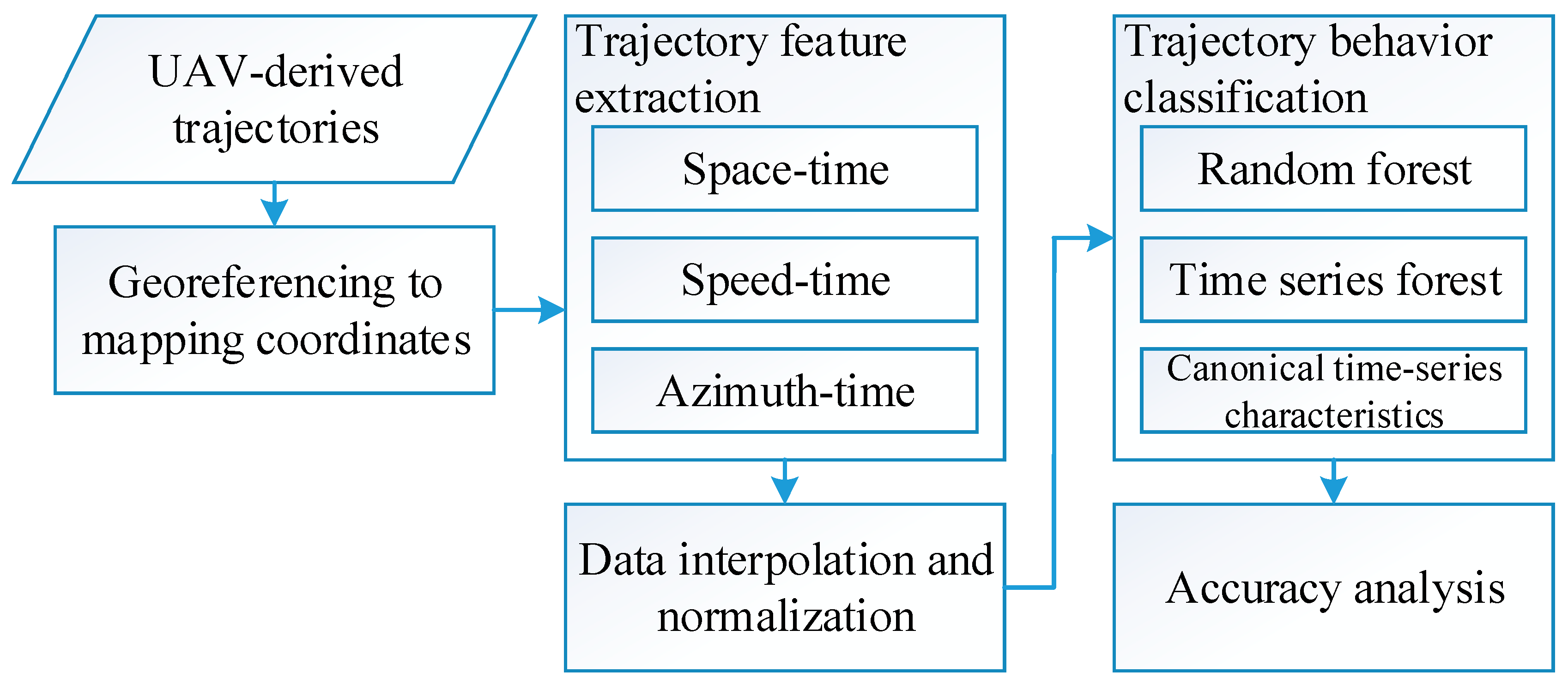
This study proposes a method for effectively classifying UAV-derived vehicle trajectories at road intersections. The workflow of the proposed method, comprising five major steps, is illustrated in Figure 1: (1) georeferencing trajectories from the image coordinate system into the real-world coordinate system; (2) extracting space–time, speed–time, and azimuth–time diagrams from trajectories; (3) aligning the data cohesively through interpolation and normalization; (4) constructing trajectory behavior classifiers; and (5) accuracy analysis.
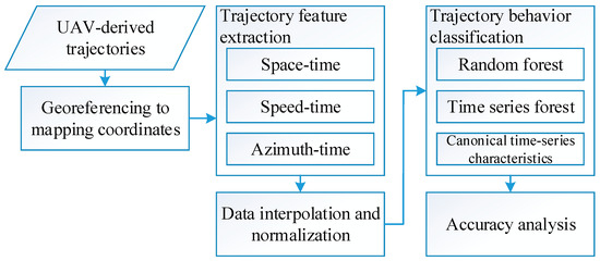
Figure 1.
Architecture of the proposed method.
2.1. Trajectory Georeferencing
Vehicle trajectories of road intersections were obtained through UAV videos, initially in the image coordinate system. To precisely calculate vehicle parameters such as the distances and directions of these trajectories, it is essential to convert the trajectories into a mapping coordinate system. This conversion ensures that the trajectory data accurately aligns with the real-world coordinate system. The first step of georeferencing is to identify the ground control points (GCPs) via a georeferenced orthoimage in the world coordinate system to ensure that they are evenly distributed across the road intersection. These GCPs are crucial for georeferencing and serve as essential anchors, enabling the accurate alignment of trajectories with the world coordinate system.
Considering that UAV videos operate through perspective projection imaging, this study adopted 2D projective transformation to convert the image coordinates into world coordinates. Equations (1) and (2) illustrate the conversion from the original image coordinates to the projected world coordinates. In the image coordinate system (u, v), u represents the sample, and v represents the line, with units in pixels. In the transformed world coordinates (E, N), E represents east, and N represents north, with units in meters. The eight parameters (a11, a12, a13, a21, a22, a23, a31, a32) represent the coefficients of the 2D projective transformation. Specifically, coefficients (a11, a12, a21, a22) correspond to scaling and rotation effects; coefficients (a13 and a23) correspond to translation; and coefficients (a31 and a32) correspond to the effect of perspective distortion. These coefficients can be determined by aligning the image coordinates with the orthoimage using GCPs and least squares adjustment. This georeferencing process converts each trajectory from image coordinates to mapping coordinates (measured in meters) using the calculated coefficients, thus making the georeferenced trajectory suitable for computing vehicle parameters with physical meaning.
where (u, v) are the image coordinates of the control points; (E, N) are the ground coordinates of the control points; and (a11, a12, a13, a21, a22, a23, a31, a32) are the coefficients of the 2D projective model.
2.2. Trajectory Feature Extraction
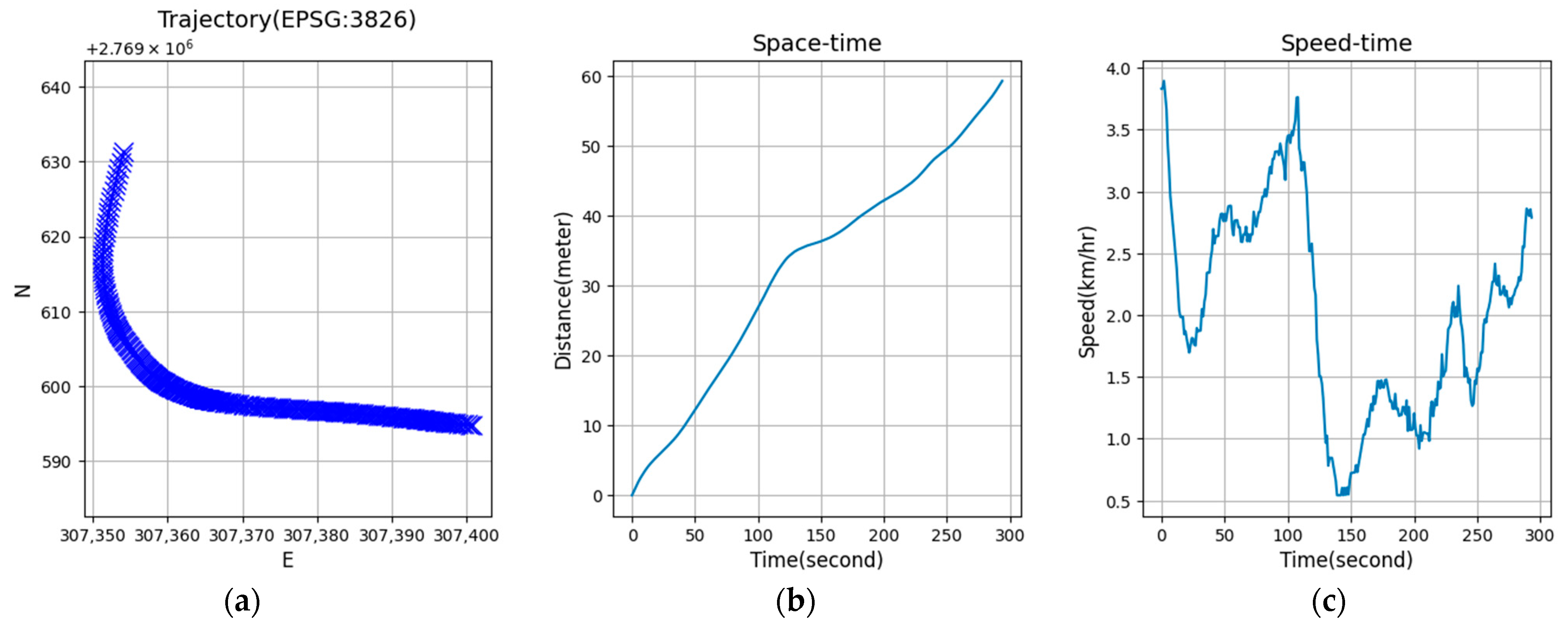
A trajectory is characterized by a series of travel times (ti) and vehicle locations (Ei, Ni) (Figure 2a). To categorize vehicle trajectories into different classes, it is necessary to extract several features. Key features such as space (distance), azimuth (direction), speed (movement), and time are vital to represent a trajectory and capture the essential aspects of vehicle spatiotemporal behavior. This study focused on using space–time, speed–time, and azimuth–time parameters to classify trajectories and improve the precision and usefulness of trajectory behavior analysis.
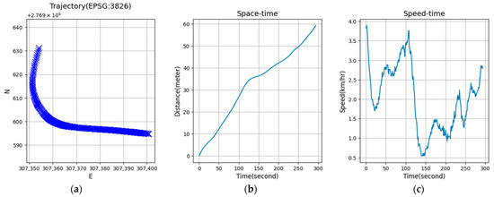
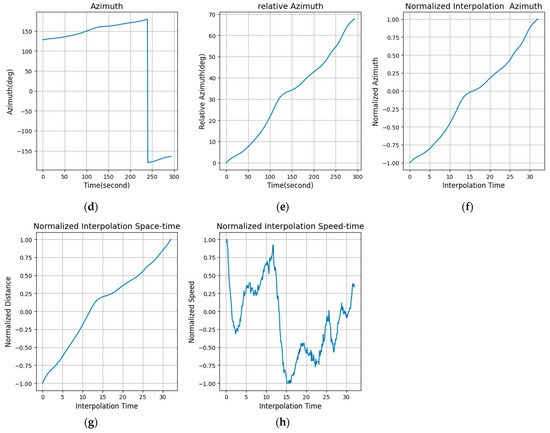
Figure 2.
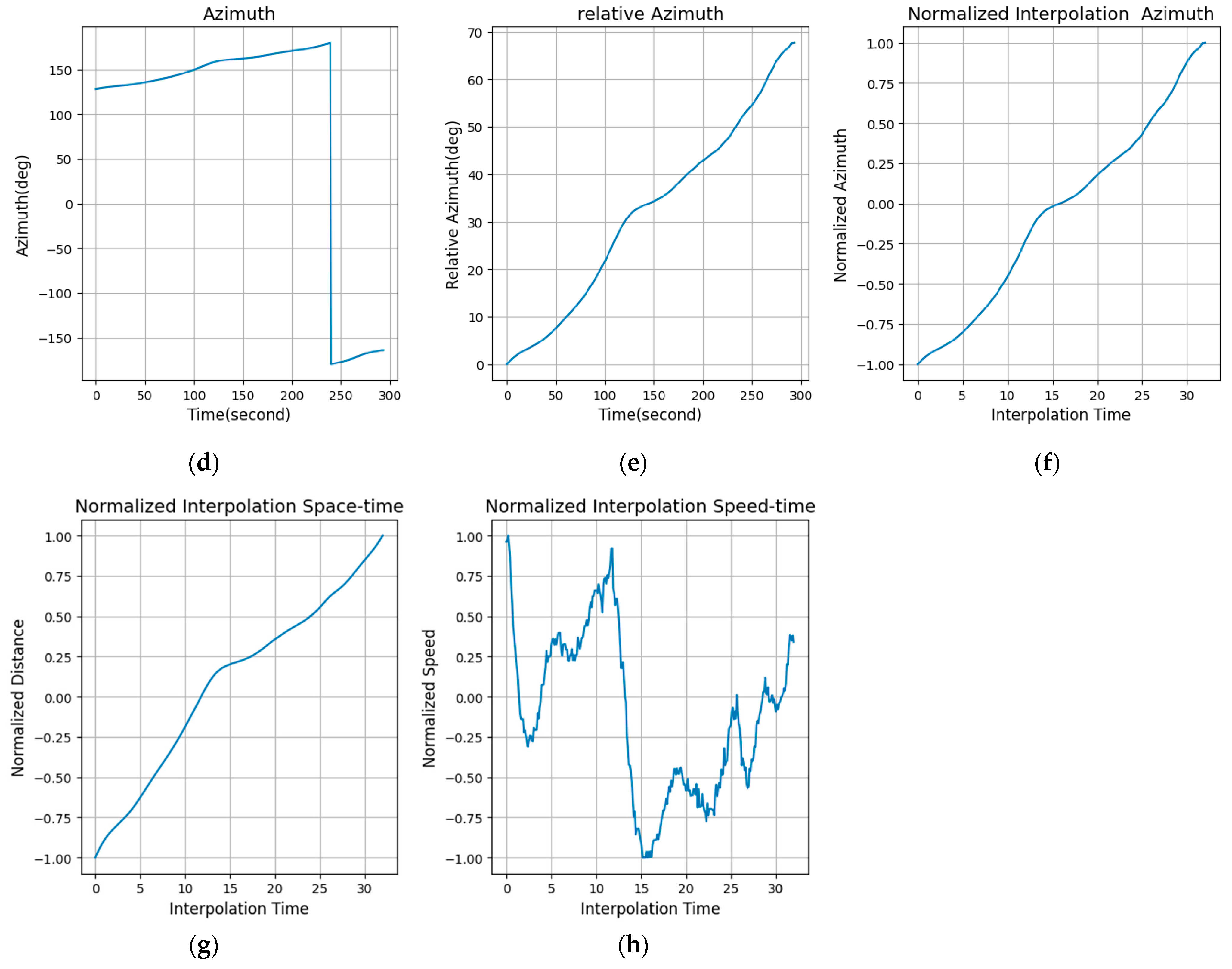
Processes of transforming a trajectory: (a) original trajectory, (b) space–time, (c) velocity, (d) original azimuth–time, (e) relative azimuth–time, (f) normalized azimuth, (g) normalized distance, and (h) normalized speed.
2.2.1. Generation of Space–Time Sequences
For transportation analysis, a space–time diagram is a graphical representation that plots vehicles’ movement along a path over time. This diagram visualizes how vehicles move and highlights their movement patterns. By depicting the distance traveled on one axis (usually the vertical axis) against time on the other (horizontal axis), analysts can observe and understand traffic flow, identify congestion points, and evaluate the efficiency of transportation systems. To generate space–time sequences from a vehicle’s trajectory, which includes its locations (Et, Nt) and timestamps (t), the cumulative traveled distance (Dt) is calculated from the starting point (E0, N0) to create the spatial component of the sequence (Equation (3)). Simultaneously, the time component (t) is derived from the timestamps, which ensures that each point in the trajectory is associated with a specific time interval. The space–time sequences are characterized by a series of travel times (t) and vehicle cumulative distances (Dt). These data points are then plotted on a graph with the x-axis representing time and the y-axis representing space (traveled distance) (Figure 2a).
where Dt is the cumulative distance; (Et, Nt) are the vehicle locations at time t; and (E0, N0) are the starting points of the vehicle.
2.2.2. Generation of Speed–Time Sequences
Speed–time sequences integrate both speed (representing space) and time aspects to provide a comprehensive view of a vehicle’s movement. This integration facilitates a more thorough understanding of how objects move considering both speed and time, providing a holistic perspective on their dynamics. Such sequences are characterized by a series of travel times (t) and the vehicle’s instantaneous speed (St). The instantaneous speed (S) can be calculated by determining the sequence distances of an object over a short time interval (Equation (4)). These data points are then plotted on a graph, with the x-axis representing time and the y-axis representing speed (Figure 2c). The speed–time diagram tracks how distance varies with time and thus helps in analyzing traffic behavior, such as differentiating whether a vehicle is stationary at a traffic light or moving.
where St is speed; Δt is the time rate; and (Dt+1 and Dt) are the traveled distances at time t + 1 and t, respectively.
2.2.3. Generation of Azimuth–Time Sequences
In trajectory behavior analysis, the calculation of the azimuth–time sequences plays a crucial role in understanding the directional changes in objects over time. The azimuth angle is a measure of a vehicle’s direction on the horizontal plane and is defined as the angle between a reference direction (i.e., geographic north) and the vehicle’s direction. The azimuth is calculated between two locations over time intervals (Equation (5)). This azimuth () serves as a representation of the directional angle from the reference direction. To understand the directional changes, the relative azimuth () is calculated from the starting azimuth () to establish a dynamic record of directional changes (Equation (6)). The azimuth–time sequence is characterized by a series of travel times (t) and relative azimuth (). Figure 2d shows an azimuth–time diagram, while Figure 2e depicts a relative azimuth–time diagram. The azimuth–time diagram focuses on directional change and thus helps in analyzing traffic behavior, such as differentiating whether a vehicle is going straight or turning in a certain direction.
where is the azimuth at time t; is the azimuth at the starting point; is the relative azimuth at time t; (Et, Nt) are the vehicle locations at time t; and (Et+1, Nt+1) are the vehicle locations at time t + 1.
2.3. Interpolation and Normalization
For various road intersections, each vehicle trajectory exhibits different travel times and distances, which leads to variability in the data length for different trajectories. This variability poses a challenge in ML for time series data analysis due to the issue of differing data lengths. To overcome this problem, this study employed linear interpolation (Equation (7)) to standardize the data lengths across all trajectories and ensure uniformity. Specifically, the data length was constrained to 32 samples (i.e., 25). Therefore, this study evenly interpolated 32 samples from the original space–time, speed–time, and azimuth–time sequences to ensure that each sequence was standardized to the same length for analysis.
Since the numerical values for space (in meters), speed (in meters per second), and azimuth (in degrees) vary, a common approach to handling heterogeneous data in ML is through data normalization. This study used the min-max scaling transformation (Equation (8)) to adjust the values of space, speed, and azimuth to a consistent range (between −1 and 1). This normalization process ensured that despite their differing units and magnitudes, these variables could be uniformly analyzed within the ML framework. In taking the azimuth–time data as an example, the process of interpolation and normalization results is depicted in Figure 2f. Here, the timestamp (x-axis) was interpolated to cover a range of 1 to 32 samples, and the azimuth data (y-axis) was normalized to a scale between −1 and 1.
where yt is the interpolated value at time t; t is the time in the interval (t1, t2); (y1, y2) are the values corresponding to t1 and t2; nt is the normalized value at time t; and (ymin, ymax) are the minimum and maximum values.
2.4. Trajectory Behavior Classification
To perform intersection-adaptive trajectory behavior classification, it is essential to combine different types of trajectory feature sequences to improve the effectiveness of the classifiers. The space–time sequences only represent the distance of vehicle motion. Incorporating additional data such as speed–time and azimuth–time sequences significantly enriches the trajectory features. Speed–time sequences are particularly suitable for identifying when a vehicle stops because its speed drops to zero during a halt, making it easy to detect stationary states. However, relying solely on speed–time sequences can be inadequate for recognizing turning movements, as these speed–time sequences do not capture directional changes. On the other hand, azimuth–time sequences, which track a vehicle’s directional changes over time, excel at identifying turning behaviors. As a vehicle turns, its azimuth, representing its direction, changes significantly, which makes it easy to identify turns. Integrating both speed–time and azimuth–time sequences thus offers a more nuanced and comprehensive approach to distinguishing between different vehicle behaviors, particularly at various intersections. In this study, following data integration, three ML classifiers, i.e., random forest (RF), time series forest (TSF), and canonical time series characteristics (Catch22), were applied to classify the trajectories into different trajectory behaviors. Finally, an accuracy analysis was performed to assess each classifier’s effectiveness in trajectory behavior classification.
2.4.1. Types of Trajectory Behaviors
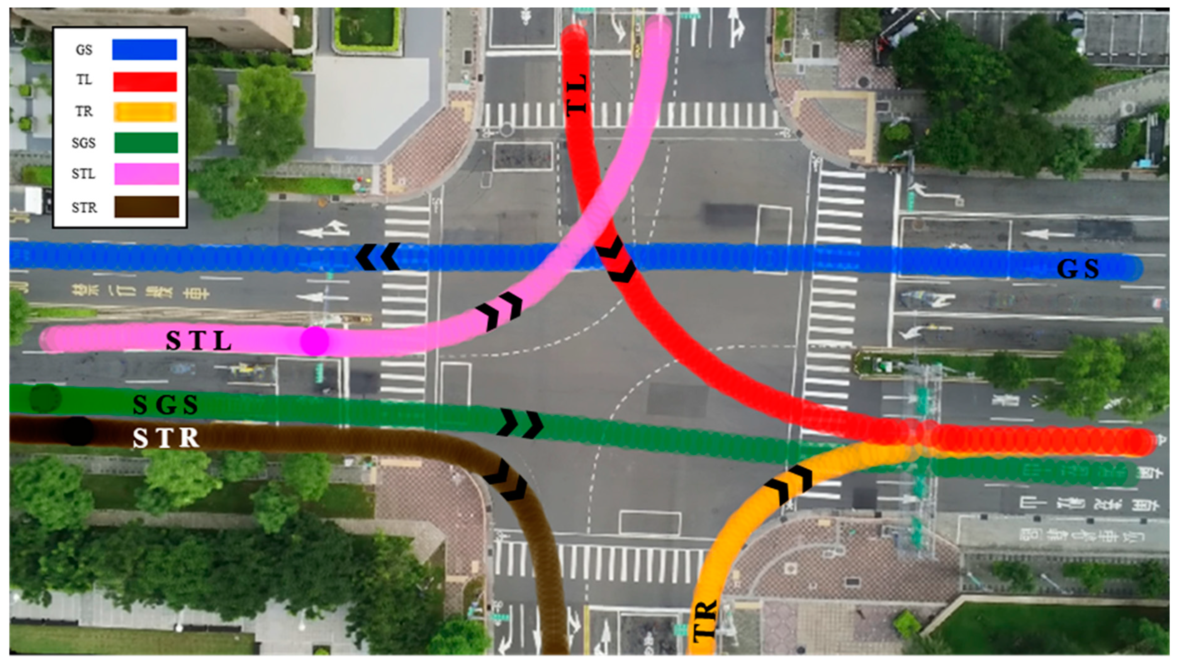
This study classified vehicle trajectories into six types based on the characteristics of intersection traffic flow: (1) go straight (GS), where vehicles follow an uninterrupted straight path through intersections without making turns; (2) turning left (TL), where vehicles execute left turns at intersections, indicating a deviation from their initial paths; (3) turning right (TR), depicting situations where vehicles make right turns at junctions, reflecting a change in their original direction; (4) stop and go straight (SGS), denoting vehicles coming to a complete stop before proceeding straight, a behavior often encountered at signalized intersections; (5) stop and turn left (STL), where vehicles halt before making a left turn at intersections; and (6) stop and turn right (STR), where vehicles make a right turn after coming to a stop at junctions, thus combining both stopping and turning behaviors. This comprehensive classification enabled a nuanced analysis of vehicle movements, with each trajectory type corresponding to specific behaviors exhibited by vehicles; this enabled us to capture diverse scenarios encountered in real-world traffic situations. For a visual representation of these trajectories, refer to Figure 3, which illustrates how each trajectory type manifests in the context of intersection traffic flow.
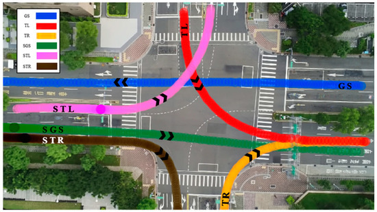
Figure 3.
Illustration of trajectory behaviors.
2.4.2. Classifier for Trajectory Behaviors
This study adopted a decision tree-based classification algorithm and investigated the impact of different feature extraction methods on vehicle trajectory behavior recognition. Three ML algorithms were utilized for trajectory behavior classification: RF [27], TSF [28], and Catch22 [29].
Random forest is an ensemble of decision trees that combines multiple decision trees to build a forest. In this ensemble, each internal node represents a decision based on a particular feature, with each leaf node representing the outcome. The final prediction is obtained by aggregating the results of each tree through voting and averaging. This ensemble prediction method proves effective in addressing the overfitting problem and enhancing the model’s precision. Random forest is based on two key sources of randomness. First, it builds a sub-dataset by randomly extracting samples from the original dataset. Each tree in the training dataset is independently generated to promote diversity. Second, when each tree is constructed, RF randomly selects a subset of features for segmentation, allowing the model to use fewer variables to deal with more complex data and features.
In time series classification problems, using the original sequences as inputs for training the RF classifier may overlook the temporal order of data points, leading to poor classification performance for problems with strong time-related dependencies. To overcome this problem, Deng et al. [28] introduced the TSF algorithm, which can be considered a random forest classifier that is tailored for time series. The time series forest algorithm is designed specifically for time series data with temporal dependencies and patterns and is essentially an extension of the RF algorithm. The TSF algorithm segments each sequence into random intervals and calculates the mean, standard deviation, and slope within each time interval, creating new data samples to train an RF classifier.
Similar to the idea of TSF, Lubba et al. [29] proposed the Catch22 algorithm to acquire dynamic changes in time series. In their study, the authors analyzed 93 time series, and 22 features were extracted for their maximum effectiveness and minimal redundancy from a pool of 4791 features. These features encompassed various aspects, such as information about distribution, linear autocorrelation, nonlinear autocorrelation, successive differences, and fluctuation analysis. This study extracted 22 features from the original sequences to create a new dataset and used it to train an RF classifier.
2.4.3. Accuracy Indices
This study evaluated the effectiveness of different time sequences of data acquired through trajectories using four evaluation metrics: accuracy, precision, recall, and F1 score. Accuracy measures the overall correctness of the model’s predictions by quantifying the proportion of correctly classified instances across all instances, taking into account both the true positives (TPs) and true negatives (TNs) (Equation (9)). Precision quantifies the number of correct classifications among instances labeled as positive in the ground truth (Equation (10)). A higher precision indicates a lower probability of false positives (FPs) by the classifier. On the other hand, recall measures the correctness of positive classifications among all positive instances in the ground truth (Equation (11)). A higher recall implies fewer instances of false negatives (FNs) by the classifier. The F1 score serves as a comprehensive metric that harmonizes precision and recall and provides an overall evaluation of the model’s performance (Equation (12)). Its value ranges from 0 to 1, with a higher F1 score indicating superior model performance. Within these metrics, TP represents the correct number of instances classified as positive when the ground truth is positive; TN represents the correct number of instances classified as negative when the ground truth is negative; FN signifies the instances falsely classified as negative when the ground truth is positive; and FP denotes the instances falsely classified as positive when the ground truth is negative.
3. Experimental Results
The proposed method for classifying trajectory behavior was tested on three UAV-derived trajectories under varying conditions. The trajectories were initially extracted using the Oriented YOLOv4 deep learning model [30]. This model enhances YOLOv4 by annotating vehicles based on their orientation (front left, front right, rear right, rear left) in a clockwise sequence. It accurately measures vehicle dimensions and positions, facilitating effective tracking using the SORT algorithm. SORT tracks vehicles by size and predicted distances between detections, ensuring efficient trajectory analysis without requiring full video content. Subsequently, manual quality control was performed to confirm their accuracy. The evaluation process was conducted in three phases. Initially, the models for trajectory behavior classification were trained and tested using the first intersection, referred to as intersection A. Next, the pre-trained models were assessed at similar intersections (intersection B) to serve as an independent validation. This intersection B is similar to intersection A, where the driving direction also remains consistent throughout the entire travel time, as shown in Figure 4a,b. Finally, the pre-trained models were subjected to evaluation at dissimilar intersections (intersection C). Intersection C is characterized by its asymmetrical road layout. As illustrated in Figure 4c with the yellow line, vehicles approaching the center of the intersection need to make a slight left turn of 16 degrees, and after passing through, they need to make a slight right turn of 20 degrees. The experiment aimed to gauge the adaptability of the pre-trained models to different intersection scenarios.
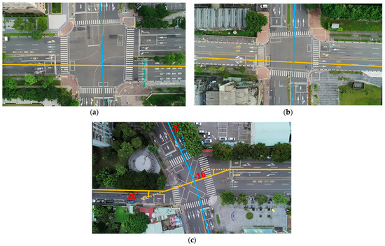
Figure 4.
Illustrations of the three intersections (the blue and yellow solid lines indicate different road center lines; the yellow dashed line indicates the extension of road center line): (a) intersection A, (b) intersection B, and (c) intersection C.
3.1. Dataset
The experiment encompassed three distinct intersections. The UAV-derived trajectories utilized in this study were provided by the Institute of Transportation, Ministry of Transportation and Communications, Taiwan. The UAV data were captured by a Parrot ANAFI drone at a rate of 9.99 frames per second, ensuring a high-frequency recording of the observed scenarios. The flying height was 80 m above the ground, and the images were captured with a 1920 × 1080 pixel resolution. After UAV data acquisition, a DL tracking technique was performed to automatically extract the vehicle trajectories at the road intersections [30]. Subsequently, a manual quality control was conducted to eliminate any incomplete tracking. The incomplete tracking refers to instances where the vehicle’s trajectory is only partially captured in the UAV’s video, either at the beginning or the end. This ensures that only vehicles present within the ground coverage for the entire duration of the video are considered. Vehicles that were already within the ground coverage at the start of the capture or those that exited before the end of the capture were excluded. Finally, each trajectory was manually categorized into six classes for accuracy analysis.
The selection of these specific locations for data capture was based on a strategic consideration of the likelihood of accidents occurring at intersections, contributing to a targeted and relevant analysis. Descriptions of the three intersections are as follows: Intersection A was divided into training and testing datasets, where 80% was allocated for training purposes, and the remaining 20% was reserved for testing. This partitioning strategy was implemented to robustly evaluate the model’s performance. The testing dataset was kept separate from the training data to ensure the reliability of the training model; this enabled an unbiased evaluation of the model’s performance on unseen data and enhanced the reliability of the training model. Intersections B and C were independent test datasets to ensure that the trained model could effectively apply to new, unseen data. Among them, intersection B was similar to the training data of intersection A, and intersection C was different from the training data of intersection A. We found it helpful to assess the model’s generalization ability. The details of each intersection are summarized in Table 1.

Table 1.
Descriptions of the three intersections.
3.2. Georeferencing
The original trajectory is located in the pixel in the image coordinates. The georeferencing process transforms the trajectory from a pixel to a meter in a world coordinate system, which is critical in accurately spatializing vehicle trajectory data and ensuring precise alignment with world coordinates. This study manually measured the transformation control points between the UAV images and the orthoimages using Taiwan e-Map. Then, a 2D projective transformation model was applied to convert the image coordinates to world coordinates. The accuracy of the georeferencing process at each intersection was evaluated through residuals VE and VN, representing the discrepancies between the converted and actual east and north coordinates, respectively. These residuals offered valuable insights into the model’s accuracy in predicting the spatial locations of trajectories. Additionally, root mean square error (RMSE) values were computed for both the east and north directions, which served as comprehensive metrics to determine the overall accuracy of the georeferencing model. The RMSE values for intersection A were 0.110 m and 0.151 m, 0.641 m, and 0.344 m for intersection B, and 0.092 m and 0.094 m for intersection C, as shown in Table 2. The largest RMSE among these was still much smaller than the lane width, suggesting acceptable errors in transforming the spatial coordinates across the intersections and thus emphasizing the efficacy of the georeferencing method in enhancing the precision of vehicle trajectory data alignment with real-world geographical coordinates. After georeferencing, all the trajectories were used to extract the space–time, speed–time, and azimuth–time sequences for classification.

Table 2.
Georeferencing performance.
3.3. Trajectory Behavior Datasets and Model Training
The vehicle trajectories were manually classified into six categories. Initially, all the trajectories were visualized in the world coordinate system. By identifying the entry and exit points (lanes), we categorized the trajectories into three primary movements: proceeding straight, turning left, and turning right, taking into account that vehicles may remain stationary near traffic lights. For every category, this study plotted the trajectory and speed in the world coordinate system. The speed’s numerical values facilitated distinguishing between the stationary vehicles and those moving near a traffic light. Further refinement allowed us to segregate the stop and go straight actions from the general go straight category. We also applied a similar methodology to delineate stop and turn left and stop and turn right behaviors. Table 3 presents the number of each class for the training, testing, and independent testing data, providing a quantitative overview for further analysis.

Table 3.
Classes of vehicle trajectory.
During the training stage, the hyperparameters for the three classifiers were based on RF and were optimized using the same parameters. The main difference between RF, TSF, and Catch22 was their approach: RF used the original trajectory as input to train an RF classifier; TSF divided the trajectory into random intervals and calculated the mean, standard deviation, and slope within each interval to create new data samples for training an RF classifier; and Catch22 extracted 22 features from the original trajectory to create a new dataset for training an RF classifier. Table 4 presents the dimensions of each classifier used in the analysis. We used 590 trajectories in the training stage. The RF classifier comprised either 32 or 64 samples, and each one was trained on 590 trajectories. The TSF classifier comprised six or eight sets. Each set comprised three components: mean, standard deviation, and slope (Deng et al., 2013). The Catch22 model utilized 22 selected features [29] as samples and was trained on 590 trajectories.

Table 4.
Dimensions of each classifier.
The configuration specified an RF ensemble with 500 decision trees using the Gini impurity criterion for splitting, and there were no restrictions on the maximum depth of the trees. The minimum number of samples required to split an internal node was 2, and the minimum number of samples required to be at a leaf node was set to 1. Bootstrap sampling was enabled, meaning that each tree was trained on a bootstrap sample of the training data. The maximum number of features considered for splitting at each node was the square root of the total number of features. The minimum number of samples required to split an internal node was set to 2, which ensured that a node had at least two samples for further splitting. Similarly, the minimum number of samples required to be at a leaf node was set to 1, which guaranteed that each leaf node contained at least one sample. Other parameters were set according to the default settings of the Scikit-learn library [31], which include not setting a specific number for the maximum leaf nodes, setting the minimum impurity decrease to 0, and using out-of-bag samples to estimate the generalization score.
To assess the computational time requirements, we used a PC equipped with an intel i7-12700F CPU and Kingston Fury 32 GB of RAM to evaluate the performance of the proposed method. The pre-processing time for each vehicle was approximately 3.38 s. The training times for the different models were as follows: random forest (RF) took 1.29 s, time series forest (TSF) took 5.43 s, and Catch22 took 2.32 s. The prediction times per vehicle were 0.00035 s for RF, 0.00445 s for TSF, and 0.00115 s for Catch22.
3.3.1. Evaluation of Test Data
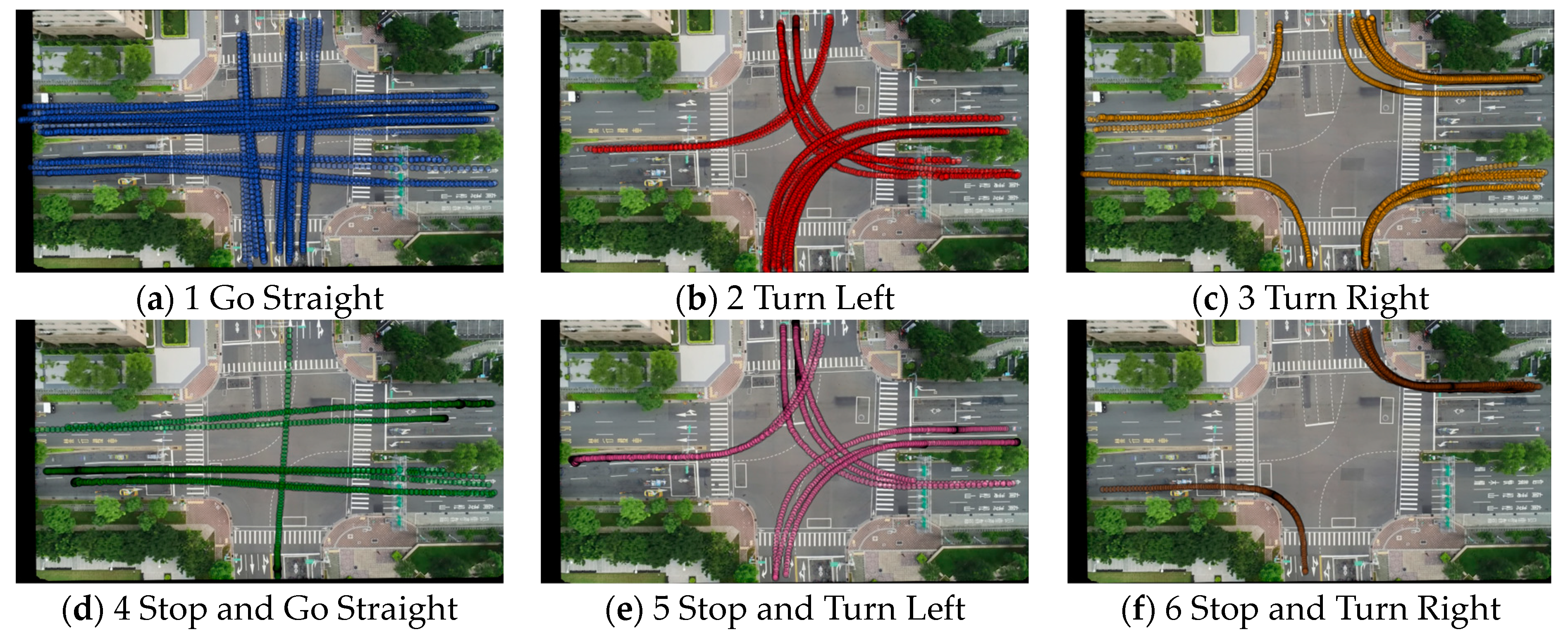
Trained models were employed to predict different sequences from the test dataset from intersection A, which had the same intersection configuration as the training data. We compared classifiers that utilized different types of information: space–time, azimuth–time, and azimuth– and speed–time, and assessed their performance differences and potential impacts. We employed standard evaluation metrics to evaluate the performance of each model, i.e., accuracy, precision, recall, and F1 score. The predicted results are summarized in Table 5. Figure 5 shows all predicted vehicle behaviors from test data. For the space–time sequences, all three classifiers showed relatively lower performance compared to the other sequences. The azimuth–time sequences demonstrated better accuracy than the space–time feature, meaning that azimuth–time was more suitable than space–time for trajectory behavior classification. The most significant performance improvements were observed when incorporating azimuth and speed information into the classifiers. The integration of azimuth– and speed–time sequences yielded higher accuracy than other sequences. The F1 scores of these three classifiers were better than 96%. Therefore, the superior performance of the predictive classifiers in the integrated sequences could be attributed to the inclusion of speed-related features. By incorporating speed data, the classifiers gained deeper insights into traffic dynamics, which enabled more accurate predictions of intersection behavior. The ability to consider speed variations enabled the classifiers to capture and adapt to traffic fluctuations effectively. Additionally, we conducted a detailed examination of the metrics for each category in integrated sequences using the RF classifier, as depicted in Table 6.

Table 5.
Overall accuracies for test data (intersection A).
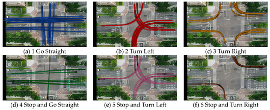
Figure 5.
Results of the test data (intersection A) classified using RF.

Table 6.
Evaluation metrics for the test data (intersection A) using azimuth– and speed–time sequences with RF.
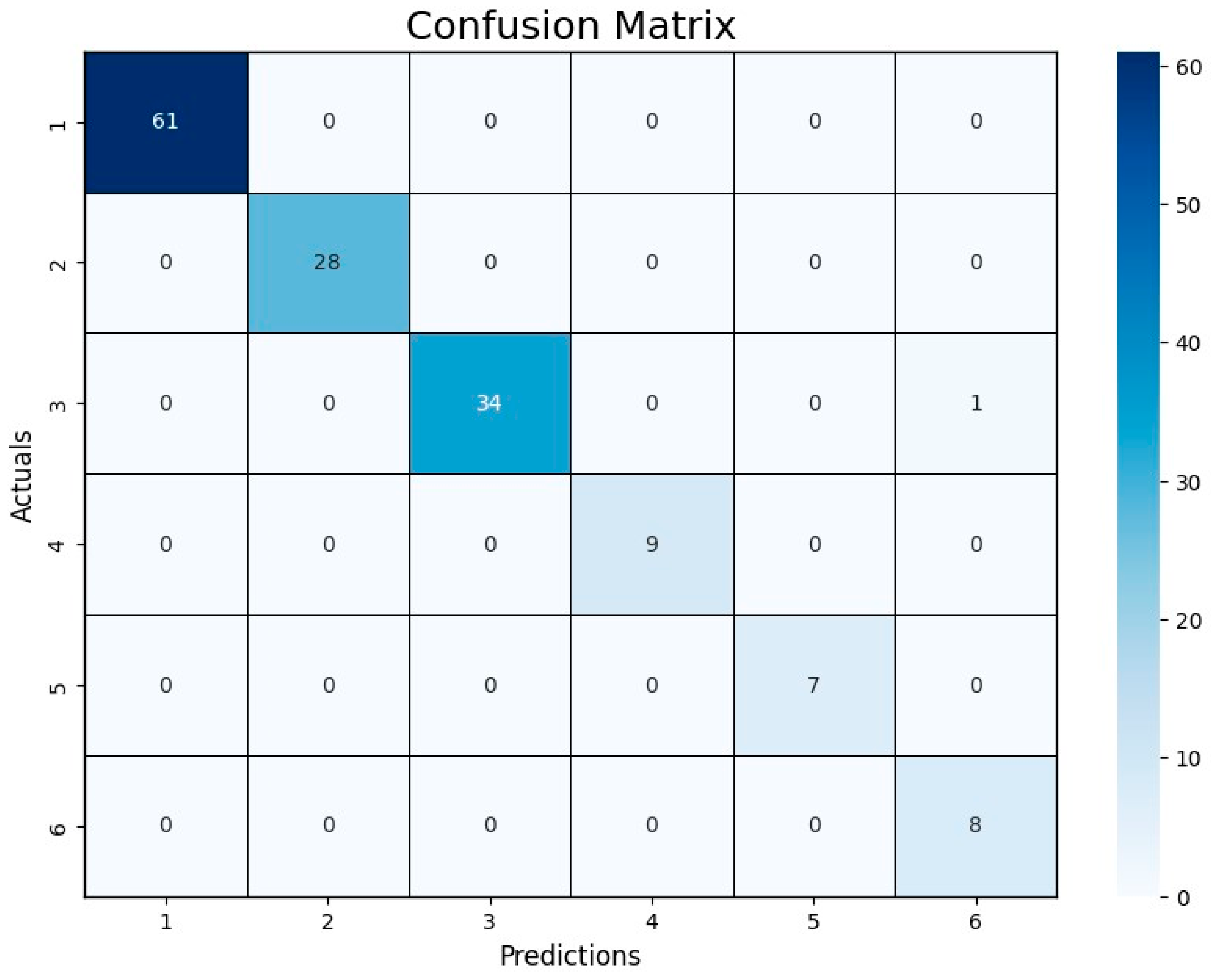
Figure 6 shows the confusion matrix of the azimuth– and speed–time sequences using RF. Misclassification was observed, where the RF classifier failed to identify instances of stopping and going straight. Further investigation was conducted on this trajectory that was incorrectly predicted by the classifier, as depicted in Figure 7. This trajectory (i.e., ID 13) was captured at the beginning of the video when the traffic signal had just turned from red to green, resulting in a brief moment of traffic congestion. Therefore, the classifier misclassified it as category 6 (i.e., stop and turn right) instead of category 3 (i.e., turn right). This scenario proved to be inherently ambiguous, and even manual identification was challenging due to varying perspectives among individuals.

Figure 6.
Confusion matrix for the test data (intersection A) using azimuth– and speed–time with RF.
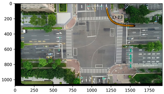
Figure 7.
Incorrectly classified trajectory at the beginning of the dataset.
3.3.2. Evaluation of Similar Intersections
The generalization ability of the ML models from intersections A to B was evaluated. Moreover, the adaptability of classifiers to a similar intersection (intersection B) was assessed by examining their performances in the three different sequences using various classifiers. The results from intersection B, detailed in Table 7, provide compelling insights into the performance.

Table 7.
Overall accuracies for intersection B.
In the space–time sequence, the three classifiers exhibited relatively lower performances than the azimuth–time sequence, which could be because only spatial movement trajectories were considered; other influencing factors were not considered, resulting in oversimplified representations of complex traffic behaviors and limited recognition capability. In contrast, the azimuth–time sequence incorporated directional information, providing insights into the trajectory’s angle relative to the reference direction. This inclusion enhanced the classifier’s ability to predict vehicle movement directions and turns accurately, thereby improving the accuracy of identifying traffic behaviors. Each classifier improved its performance, especially Catch22, and emerged as the top performer in this scenario, achieving an F1 score of 91.90%. These results underscore the adaptability and effectiveness of Catch22 in capturing the nuances of the azimuth–time sequence.
In integrating azimuth–time and speed–time sequences, both the RF and TSF models demonstrated a significant improvement in overall performance. However, Catch22 experienced a decline in performance, with notable drops in the F1 score compared to its performance in the azimuth–time sequence. Particularly noteworthy was TSF’s leading position, which achieved a remarkable F1 score of 97.37%. RF and Catch22 exhibited significantly inferior performances compared to TSF, with F1 scores consistently near 83%. In consideration of the preceding analysis, Table 8 provides the predicted results for each category at intersection B in the azimuth– and speed–time sequence using the TSF classifier. Figure 8 shows all predicted vehicle behaviors from intersection B. The F1 score for the majority of the categories was above 90%, indicating that the TSF struck a good balance between precision and recall and demonstrating its robust performance in multi-category classification scenarios. The results indicate that TSF outperformed RF in the overall performance, possibly because the RF classifier, trained directly on the original sequences, did not consider the temporal order of data points. However, the TSF algorithm implicitly considered the temporal order of the data points through random time intervals, resulting in better classification outcomes. This suggests that temporal sequencing is crucial in trajectory behavior classification.

Table 8.
Evaluation metrics for intersection B using azimuth– and speed–time sequences with TSF.

Figure 8.
Results of intersection B classified using TSF.
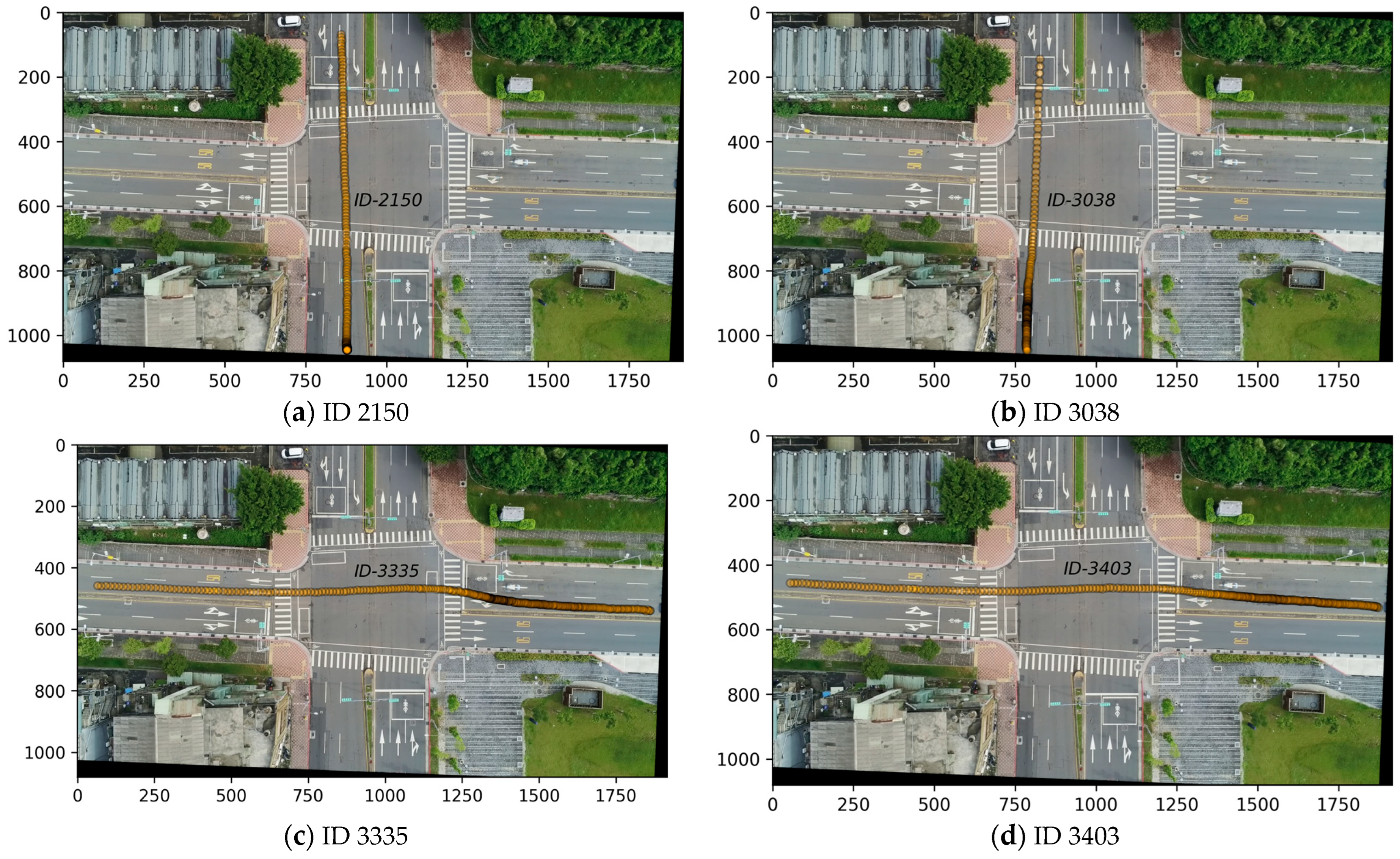
Upon closer examination of Figure 9, the primary concern is evidently the potential misclassification of the stop-and-wait behaviors. Moreover, when comparing categories, category 4 exhibited a recall of 86.15%, which was comparatively lower than those of the other categories. This implies that the model might have missed a portion of TP instances within this category. Specifically, instances involving ID 2150 and ID 3038 were erroneously classified as category 1, despite their ground truth belonging to category 4. This misclassification could be because traffic jams were encountered at the end of these trajectories, causing the vehicles to move very slowly (not stationary), as shown at the bottom of Figure 10a,b. Additionally, instances involving ID 3335 and ID 3403 encountered vehicles in front waiting at the left traffic signal while the right lane still had traffic, causing them to decelerate and momentarily pause. Determining whether these instances resulted due to stopping for traffic light behavior was a challenge due to complex traffic dynamics. Further definition of the characteristics and nuances of category 4 instances is necessary to enhance the classification accuracy and address potential misclassifications.

Figure 9.
Confusion matrix for intersection B using azimuth– and speed–time with TSF.
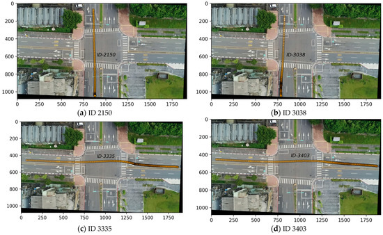
Figure 10.
Incorrectly identified trajectories in category 4. (a,b) IDs 2150 and 3038, misclassification of trajectories due to traffic jams. (c,d) IDs 3335 and 3403, traffic delay due to left turn signal wait.
3.3.3. Evaluation of Dissimilar Intersections
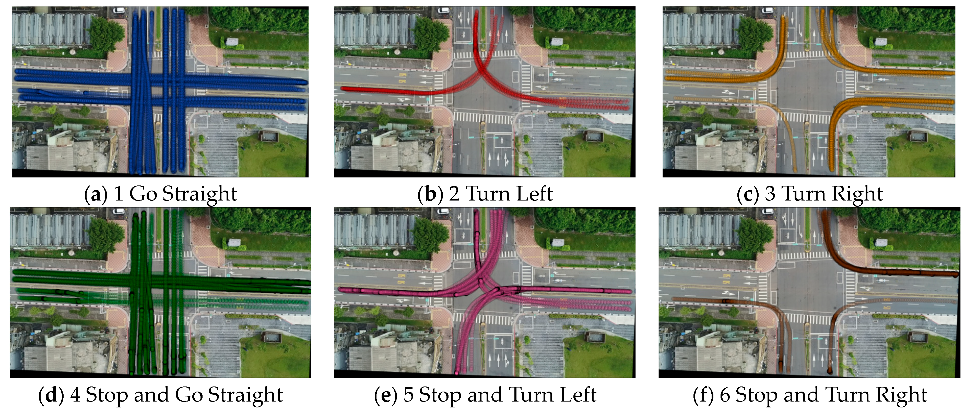
The evaluation of dissimilar intersections offers valuable information on the adaptability of trained classifiers across diverse traffic scenarios; therefore, we conducted a further investigation to determine whether variations in the intersection characteristics influenced the classifier’s response to different trajectory transformations. We utilized an intersection (intersection C) that was significantly different from the training data (intersection A) to evaluate these models, and the results are presented in Table 9. Figure 11 shows all predicted vehicle behaviors from intersection C.

Table 9.
Overall accuracies for intersection C.
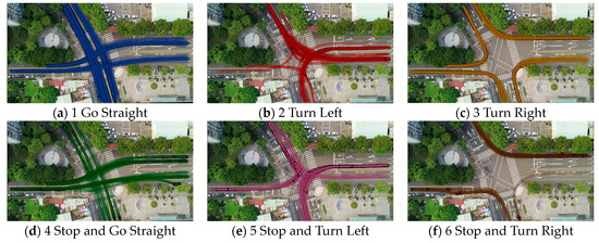
Figure 11.
Results of intersection C classified using TSF: (a) go straight; (b) turn left; (c) turn right; (d) stop and go straight; (e) stop and turn left; (f) stop and turn right.
In the space–time sequence, all models exhibited relatively lower accuracy, precision, recall, and F1 scores. As mentioned above, this could be because a limited number of features was considered. In the azimuth–time sequence, adding the azimuth information, representing the angle of the trajectory relative to a reference direction, once again reaffirmed its enhancement in accurately predicting vehicle movement directions and turns. Catch22 consistently provided better results than the other two methods and yielded an F1 score of 81.13%. Through comparing these results with the previously discussed outcomes for similar intersection results (Table 5 and Table 7), it was found that dissimilar intersections evidently had a significant impact on the performances of the classifiers. This result further underscores the potential limitations of azimuth–time in handling diverse dissimilar intersections. In the azimuth– and speed–time sequence, all classifiers demonstrated significant improvements compared to azimuth–time alone, especially the RF and TSF classifiers. The TSF showed notable improvements in accuracy (56.95–93.95%), recall (68.56–92.35%), and F1 score (58.03–90.19%), indicating its robustness in capturing complex patterns associated with combined azimuth and speed information.
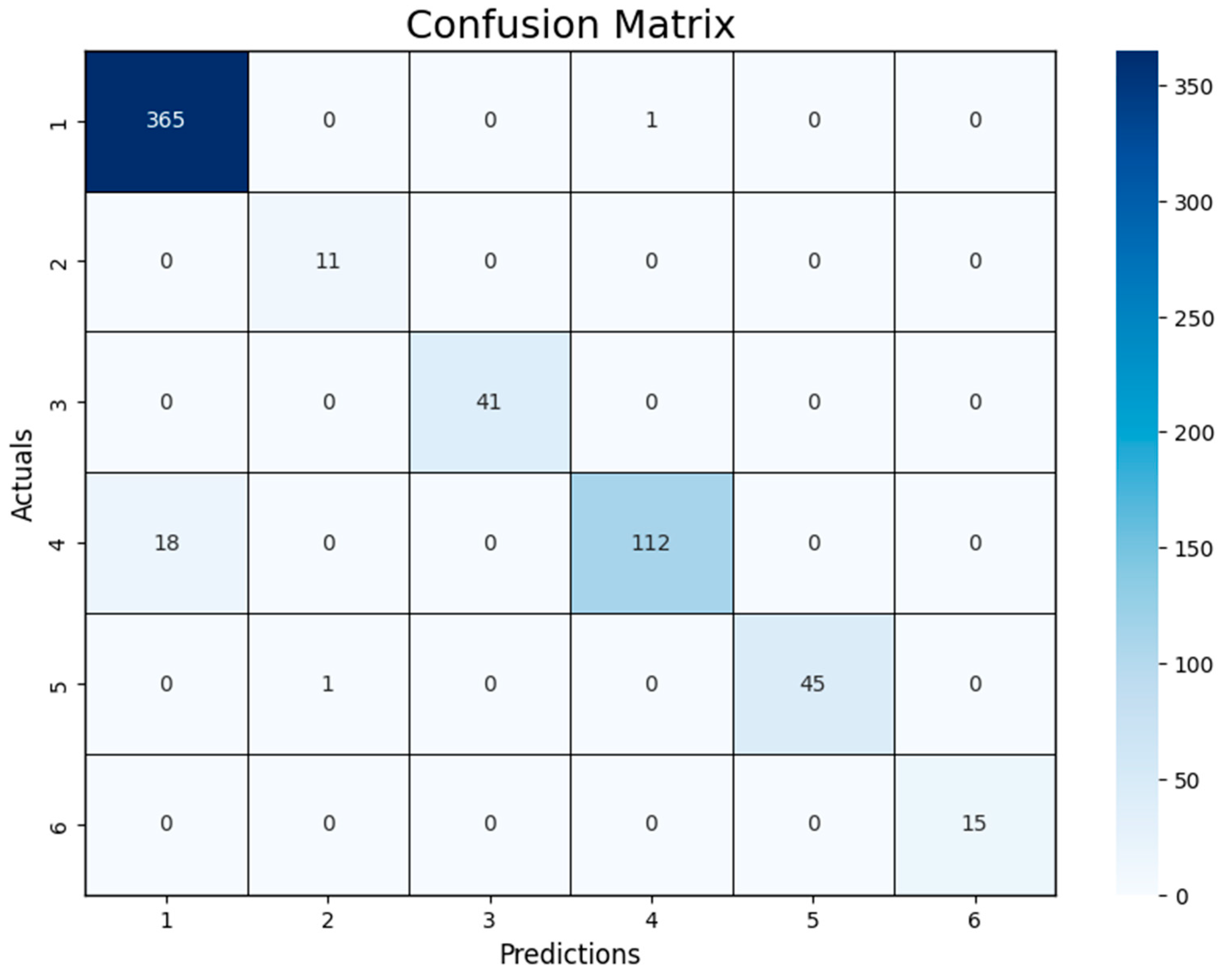
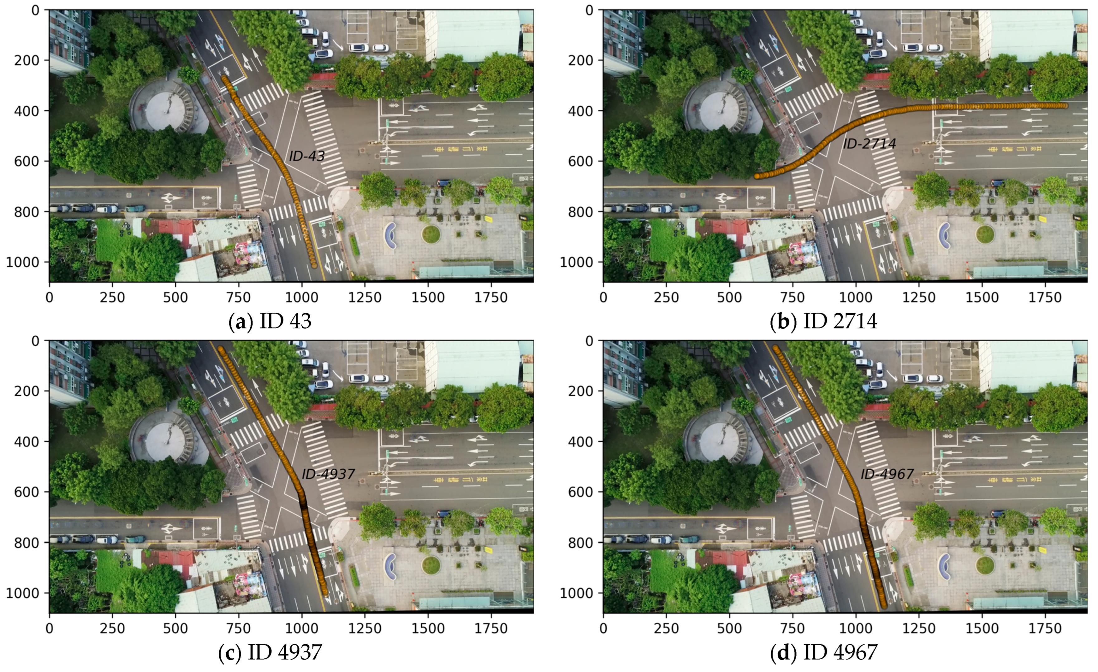
The incorporation of the speed feature had a positive impact on the overall performances of these classifiers. The model’s performance across distinct categories was notable, which is depicted in Table 10. Most of the categories stood out with high accuracy, indicating the model’s exceptional accuracy in identifying and capturing instances within these patterns. Category 2 showed the lowest F1 score (82.76%) among all the categories, indicating challenges for the model in accurately identifying all instances. This could imply that certain instances within this category were either missed or misclassified by the model, leading to an incomplete representation of the TP instances. Therefore, upon further examination of the confusion matrix Figure 12, it became evident that the primary issue was the misclassification of stop-and-wait behaviors. Figure 13 shows the vehicles that were incorrectly classified. Figure 13a,b show that vehicles moving straight ahead were mistakenly predicted as turning vehicles. This discrepancy primarily arose due to significant differences between this intersection and the training data, resulting in classification confusion. Additionally, Figure 13c,d depict situations where there were no red lights. Nevertheless, due to chaotic traffic conditions resulting in vehicles decelerating and stopping in the middle of the intersection, the model predicted the presence of stopping behavior. However, while this aspect of misclassification decreased the overall accuracy, it unexpectedly revealed the detection of traffic anomalies.

Table 10.
Evaluation metrics for intersection C using azimuth– and speed–time sequences with TSF.
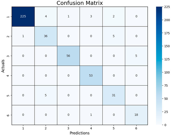
Figure 12.
Confusion matrix for intersection C using azimuth– and speed–time with TSF.
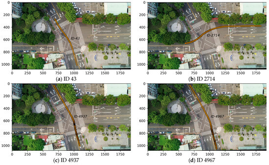
Figure 13.
Incorrectly identified trajectories in intersection C. (a,b) IDs 43 and 2714, incorrect classification due sudden change in direction; (c,d) ID 4937 and 4967, incorrect classification due to traffic jams.
3.3.4. Comparison of Different Sequences
A comprehensive comparative analysis of the space–time, azimuth–time, and integrated (azimuth– and speed–time) sequences across multiple intersections (i.e., intersections A, B, and C) was conducted. The assessment employed TSF, Catch22, and RF classifiers to evaluate the performance in terms of precision, recall, and F1 score.
In the space–time sequence, the inability to achieve proper training due to insufficient information across the experimental regions resulted in poor predictions across all classifiers, highlighting the challenge of adequately capturing crucial features during training. Consequently, in complex traffic scenarios, solely relying on space–time information may not sufficiently capture the diversity and variability of driving behaviors. In the azimuth–time sequence, Catch22 consistently demonstrated relatively high performance in precision, recall, and F1 score across all three intersections. Despite its commendable performance, there remains room for improvement, especially for the RF, which tended to exhibit a comparatively weaker performance. On the other hand, in the integrated sequences (azimuth– and speed–time), each classifier performed above a satisfactory level. Notably, TSF consistently outperformed others in terms of precision, recall, and F1 score. Furthermore, compared to the scenarios without speed information, the results of this sequence with speed information exhibited heightened stability and consistently achieved higher accuracy. Even in scenarios that were substantially different from the training data, such as intersection C, the azimuth– and speed–time sequence continued to yield stable performance and demonstrated adaptability and reliability in handling variations. This incorporation of speed information significantly contributed to enhancing the predictive accuracy and robustness of the trajectory prediction models. Furthermore, the TSF classifier consistently exhibited robust performance across diverse scenarios, emphasizing the importance of integrating comprehensive data dimensions to ensure reliability in handling intricate trajectory patterns.
3.3.5. Summary
Evaluation of test data: An evaluation of the test data revealed that the best results were obtained by integrating azimuth and speed information into the classifiers. Specifically, the integrated azimuth– and speed–time sequences yielded the highest accuracy and F1 scores among the classifiers. The RF classifier achieved an accuracy of 99.32%, a precision of 98.14%, a recall of 99.52%, and an F1 score of 98.78%. These results indicate that the inclusion of speed-related features significantly enhanced the classifiers’ ability to accurately predict intersection behavior by providing deeper insights into traffic dynamics.
Similar intersections: In the evaluation of similar intersections, the integration of azimuth–time and speed–time sequences demonstrated the best results. The TSF classifier emerged as the top performer, achieving an impressive F1 score of 97.37%. This performance surpassed that of both the RF and Catch22 classifiers, which had F1 scores consistently near 83%. The TSF classifier’s superior performance is attributed to its consideration of the temporal order of data points, resulting in more accurate classification outcomes. While Catch22 performed well with the azimuth–time sequence, achieving an F1 score of 91.90%, it experienced a decline when speed data were also incorporated. Thus, the TSF classifier is identified as the most effective model for trajectory behavior classification in this study, especially when incorporating both azimuth and speed information.
Dissimilar intersections: In the evaluation of dissimilar intersections, the integration of azimuth– and speed–time sequences yielded the most significant improvements in the classifier performance. The TSF classifier stood out with notable increases in accuracy (from 56.95% to 93.95%), recall (from 68.56% to 92.35%), and F1 score (from 58.03% to 90.19%), highlighting its robustness in handling complex patterns associated with combined azimuth and speed information. Catch22 consistently performed well with an F1 score of 81.13% in the azimuth–time sequence but showed limitations in dissimilar intersections compared to TSF. Overall, TSF demonstrated superior adaptability to diverse intersection conditions, emphasizing its effectiveness in trajectory behavior classification across varied scenarios when incorporating both azimuth and speed data.
Based on the evaluation across three different intersections, the integration of azimuth and speed information for TSF consistently showed the best performance among the evaluated classifiers. Predicting vehicle behavior is pivotal in enhancing intersection transportation management. Through accurately analyzing vehicle movements based on observation data, traffic systems can dynamically adjust signal timings, manage congestion, and prevent collisions. For example, Zhang et al. [32] integrated both turning intentions and prior trajectories to predict vehicle movements at intersections. This prediction capability allows for real-time adjustments in traffic management systems, such as adaptive traffic signals and lane management. Another application is in autonomous driving; vehicle motion prediction significantly improves autonomous vehicles’ understanding of their dynamic environments, enhancing both safety and efficiency [33].
4. Conclusions and Future Works
This study proposes a scheme for UAV-derived trajectory behavior classification. It employed trajectory transformation, converting original trajectories into space–time, speed–time, and azimuth–time sequences for each vehicle’s trajectory. Thereafter, this study normalized the data to ensure uniformity in the data formats across all sequences for ML classification. Three classifiers, RF, TSF, Catch22, were used to distinguish the trajectories into six categories. Finally, the three intersections were selected to evaluate accuracies.
The experimental results show that trajectory behavior classification in various intersections achieved an accuracy of over 90%. Upon comparing the three different sequences, integrating azimuth–time and speed–time sequences outperformed the traditional space–time sequence. The directional and movement information from azimuth–time and speed–time sequences offered better interpretation for various trajectory behaviors. Upon comparing the three different classifiers, it was found that TSF consistently exhibited robust performance when integrating speed data. This integration demonstrates TSF’s efficiency in extracting valuable features, contributing to its reliability in handling intricate trajectory patterns. When incorporating direction and speed information, the advantages of the azimuth– and speed–time scenarios were evident with the consistently high performance of TSF in terms of precision, recall, and F1 score.
This study performed well at symmetrical and neat intersections, which are characterized by regular grid layouts where vehicles typically move in straight lines or make standard turns without complex maneuvers. However, there were misclassifications in determining stop-and-go at non-symmetrical intersections. Non-symmetrical intersections have irregular layouts and varied traffic flow patterns, such as intersections where vehicles must navigate multiple turns or asymmetrical lanes, making accurate classification more challenging. Nevertheless, these results still prove the superiority of the proposed trajectory behavior classification method over traditional monitoring approaches. Future work will focus on improving the accuracy of trajectory behavior analysis at non-symmetrical intersections and also emphasize analyzing the traffic flow at intersections based on extracted trajectory behaviors. Although the prediction time for vehicle behaviors is quite fast (i.e., 0.00035 s per vehicle), the input trajectory still relies on UAV photogrammetry and deep learning processes. The processing time for tracking using deep learning is relatively slower than the processing time for analyzing trajectory behaviors using machine learning. Therefore, this study focused on trajectory analysis in a post-processing context rather than real-time implementation. Future work will focus on GPU deployment to improve computational performance for ‘near real-time’ analysis.
Author Contributions
Tee-Ann Teo conceptualized the overall research, designed the methodologies and experiments, and wrote the majority of the manuscript. Min-Jhen Chang and Tsung-Han Wen contributed to the implementation of the proposed algorithms, conducted the experiments, and performed the data analyses. All authors have read and agreed to the published version of the manuscript.
Funding
This research was partially funded by National Science and Technology Council, Taiwan, under the grant number NSTC 112-2121-M-A49-003.
Data Availability Statement
The data presented in this study are available on request from the corresponding author due to copyright and government regulations.
Acknowledgments
The authors would like to thank Ministry of Transportation and Communications (MOTC) of Taiwan for providing UAV-derived trajectory dataset.
Conflicts of Interest
The authors declare no conflicts of interest.
References
- Guo, H.; Chen, X.; Yu, M.; Uradziński, M.; Cheng, L. The usefulness of sensor fusion for unmanned aerial vehicle indoor positioning. Int. J. Intell. Unmanned Syst. 2024, 12, 1–18. [Google Scholar] [CrossRef]
- Yang, X. Unmanned visual localization based on satellite and image fusion. J. Phys. Conf. Ser. 2019, 1187, 042026. [Google Scholar] [CrossRef]
- Battiston, A.; Sharf, I.; Nahon, M. Attitude estimation for collision recovery of a quadcopter unmanned aerial vehicle. Int. J. Robot. Res. 2019, 38, 1286–1306. [Google Scholar] [CrossRef]
- Lee, H.; Yoon, J.; Jang, M.S.; Park, K.J. A robot operating system framework for secure UAV communications. Sensors 2021, 21, 1369. [Google Scholar] [CrossRef] [PubMed]
- Li, Y. Short-term prediction of motorway travel time using ANPR and loop data. J. Forecast. 2008, 27, 507–517. [Google Scholar] [CrossRef]
- Kong, Q.J.; Li, Z.; Chen, Y.; Liu, Y. An approach to urban traffic state estimation by fusing multisource information. IEEE Trans. Intell. Transp. Syst. 2009, 10, 499–511. [Google Scholar] [CrossRef]
- Kurniawan, J.; Syahra, S.G.; Dewa, C.K. Traffic congestion detection: Learning from CCTV monitoring images using convolutional neural network. Procedia Comput. Sci. 2018, 144, 291–297. [Google Scholar] [CrossRef]
- Guo, Y.; Wu, C.; Du, B.; Zhang, L. Density Map-based vehicle counting in remote sensing images with limited resolution. ISPRS J. Photogramm. Remote Sens. 2022, 189, 201–217. [Google Scholar] [CrossRef]
- Barmpounakis, E.; Geroliminis, N. On the new era of urban traffic monitoring with massive drone data: The pNEUMA large-scale field experiment. Transp. Res. Part C Emerg. Technol. 2020, 111, 50–71. [Google Scholar] [CrossRef]
- Guido, G.; Gallelli, V.; Rogano, D.; Vitale, A. Evaluating the accuracy of vehicle tracking data obtained from Unmanned Aerial Vehicles. Int. J. Transp. Sci. Technol. 2016, 5, 136–151. [Google Scholar] [CrossRef]
- Rajagede, R.A.; Dewa, C.K. Recognizing Arabic letter utterance using convolutional neural network. In Proceedings of the 2017 18th IEEE/ACIS International Conference on Software Engineering, Artificial Intelligence, Networking and Parallel/Distributed Computing (SNPD), Kanazawa, Japan, 26–28 June 2017; IEEE: Piscataway, NJ, USA, 2017; pp. 181–186. [Google Scholar]
- Berghaus, M.; Lamberty, S.; Ehlers, J.; Kalló, E.; Oeser, M. Vehicle trajectory dataset from drone videos including off-ramp and congested traffic–Analysis of data quality, traffic flow, and accident risk. Commun. Transp. Res. 2024, 4, 100133. [Google Scholar] [CrossRef]
- Xu, Z.; Yuan, J.; Yu, L.; Wang, G.; Zhu, M. Machine Learning-Based Traffic Flow Prediction and Intelligent Traffic Management. Int. J. Comput. Sci. Inf. Technol. 2024, 2, 18–27. [Google Scholar] [CrossRef]
- Ke, R.; Li, Z.; Tang, J.; Pan, Z.; Wang, Y. Real-time traffic flow parameter estimation from UAV video based on ensemble classifier and optical flow. IEEE Trans. Intell. Transp. Syst. 2018, 20, 54–64. [Google Scholar] [CrossRef]
- Biswas, D.; Su, H.; Wang, C.; Stevanovic, A. Speed estimation of multiple moving objects from a moving UAV platform. ISPRS Int. J. Geo-Inf. 2019, 8, 259. [Google Scholar] [CrossRef]
- Ke, R.; Feng, S.; Cui, Z.; Wang, Y. Advanced framework for microscopic and lane-level macroscopic traffic parameters estimation from UAV video. IET Intell. Transp. Syst. 2020, 14, 724–734. [Google Scholar] [CrossRef]
- Khan, M.A.; Ectors, W.; Bellemans, T.; Janssens, D.; Wets, G. Unmanned aerial vehicle-based traffic analysis: A case study for shockwave identification and flow parameters estimation at signalized intersections. Remote Sens. 2018, 10, 458. [Google Scholar] [CrossRef]
- Kaufmann, S.; Kerner, B.S.; Rehborn, H.; Koller, M.; Klenov, S.L. Aerial observations of moving synchronized flow patterns in over-saturated city traffic. Transp. Res. Part C Emerg. Technol. 2018, 86, 393–406. [Google Scholar] [CrossRef]
- Liu, P.; Kurt, A.; Özgüner, Ü. Trajectory prediction of a lane changing vehicle based on driver behavior estimation and classification. In Proceedings of the 17th international IEEE conference on intelligent transportation systems (ITSC), Qingdao, China, 8–11 October 2014; IEEE: Piscataway, NJ, USA, 2014; pp. 942–947. [Google Scholar]
- Zhang, M.; Fu, R.; Morris, D.D.; Wang, C. A framework for turning behavior classification at intersections using 3D LIDAR. IEEE Trans. Veh. Technol. 2019, 68, 7431–7442. [Google Scholar] [CrossRef]
- Chen, S.; Xue, Q.; Zhao, X.; Xing, Y.; Lu, J.J. Risky driving behavior recognition based on vehicle trajectory. Int. J. Environ. Res. Public Health 2021, 18, 12373. [Google Scholar] [CrossRef]
- Xiao, H.; Wang, C.; Li, Z.; Wang, R.; Bo, C.; Sotelo, M.A.; Xu, Y. UB-LSTM: A trajectory prediction method combined with vehicle behavior recognition. J. Adv. Transp. 2020, 2020, 8859689. [Google Scholar] [CrossRef]
- Zhang, H.; Fu, R. An Ensemble Learning–Online Semi-Supervised Approach for Vehicle Behavior Recognition. IEEE Trans. Intell. Transp. Syst. 2021, 23, 10610–10626. [Google Scholar] [CrossRef]
- Saeed, W.; Saleh, M.S.; Gull, M.N.; Raza, H.; Saeed, R.; Shehzadi, T. Geometric features and traffic dynamic analysis on 4-leg intersections. Int. Rev. Appl. Sci. Eng. 2024, 15, 171–188. [Google Scholar] [CrossRef]
- Razali, H.; Mordan, T.; Alahi, A. Pedestrian intention prediction: A convolutional bottom-up multi-task approach. Transp. Res. Part C Emerg. Technol. 2021, 130, 103259. [Google Scholar] [CrossRef]
- Zhou, Y.; Tan, G.; Zhong, R.; Li, Y.; Gou, C. PIT: Progressive interaction transformer for pedestrian crossing intention prediction. IEEE Trans. Intell. Transp. Syst. 2023, 24, 14213–14225. [Google Scholar] [CrossRef]
- Breiman, L. Random forests. Mach. Learn. 2001, 45, 5–32. [Google Scholar] [CrossRef]
- Deng, H.; Runger, G.; Tuv, E.; Vladimir, M. A time series forest for classification and feature extraction. Inf. Sci. 2013, 239, 142–153. [Google Scholar] [CrossRef]
- Lubba, C.H.; Sethi, S.S.; Knaute, P.; Schultz, S.R.; Fulcher, B.D.; Jones, N.S. CATCH22: CAnonical Time-series CHaracteristics: Selected through highly comparative time-series analysis. Data Min. Knowl. Discov. 2019, 33, 1821–1852. [Google Scholar] [CrossRef]
- Su, C.W.; Wong, W.K.I.; Chang, K.K.; Yeh, T.H.; Kung, C.C.; Huang, M.C.; Wen, C.S. Pedestrian And Vehicle Trajectory Extraction Based on Aerial Images. Transp. Plan. J. 2020, 49, 235–258. [Google Scholar]
- Pedregosa, F.; Varoquaux, G.; Gramfort, A.; Michel, V.; Thirion, B.; Grisel, O.; Blondel, M.; Prettenhofer, P.; Weiss, R.; Dubourg, V.; et al. Scikit-learn: Machine learning in Python. J. Mach. Learn. Res. 2011, 12, 2825–2830. [Google Scholar]
- Zhang, T.; Song, W.; Fu, M.; Yang, Y.; Wang, M. Vehicle motion prediction at intersections based on the turning intention and prior trajectories model. IEEE/CAA J. Autom. Sin. 2021, 8, 1657–1666. [Google Scholar] [CrossRef]
- Huang, R.; Zhuo, G.; Xiong, L.; Lu, S.; Tian, W. A Review of Deep Learning-Based Vehicle Motion Prediction for Autonomous Driving. Sustainability 2023, 15, 14716. [Google Scholar] [CrossRef]
Disclaimer/Publisher’s Note: The statements, opinions and data contained in all publications are solely those of the individual author(s) and contributor(s) and not of MDPI and/or the editor(s). MDPI and/or the editor(s) disclaim responsibility for any injury to people or property resulting from any ideas, methods, instructions or products referred to in the content. |
© 2024 by the authors. Licensee MDPI, Basel, Switzerland. This article is an open access article distributed under the terms and conditions of the Creative Commons Attribution (CC BY) license (https://creativecommons.org/licenses/by/4.0/).

