Abstract
Human mobility data are crucial for transportation planning and congestion management. However, challenges persist in accessing and using raw mobility data due to privacy concerns and data quality issues such as redundancy, missing values, and noise. This research introduces an innovative GIS-based framework for creating individual-level long-term spatio-temporal mobility data at a city scale. The methodology decomposes and represents individual mobility by identifying key locations where activities take place and life patterns that describe transitions between these locations. Then, we present methods for extracting, representing, and generating key locations and life patterns from large-scale human mobility data. Using long-term mobility data from Shanghai, we extract life patterns and key locations and successfully generate the mobility of 30,000 virtual users over seven days in Shanghai. The high correlation (R² = 0.905) indicates a strong similarity between the generated data and ground-truth data. By testing the combination of key locations and life patterns from different areas, the model demonstrates strong transferability within and across cities, with relatively low RMSE values across all scenarios, the highest being around 0.04. By testing the representativeness of the generated mobility data, we find that using only about 0.25% of the generated individuals’ mobility is sufficient to represent the dynamic changes of the entire urban population on a daily and hourly resolution. The proposed methodology offers a novel tool for generating long-term spatiotemporal mobility patterns at the individual level, thereby avoiding the privacy concerns associated with releasing real data. This approach supports the broad application of individual mobility data in urban planning, traffic management, and other related fields.
1. Introduction
The widespread adoption of smartphones and the availability of signaling data from these devices have provided detailed and accurate information on individual mobility characteristics [1]. This type of data represents users’ daily travel behaviors, playing a crucial role in aspects such as residential travel surveys and transportation demand forecasting [2]. Through the fusion and analysis of multisource data, the precise analysis of individual travel characteristics can be achieved, facilitating multiscale spatio-temporal transportation demand analysis and prediction [3,4]. Human mobility data are of significant importance for applications in urban transportation planning, the prediction and simulation of infectious disease spread, crime risk assessment, crowd gathering warnings, and evacuation planning [5,6].
Despite the ease of collecting large-scale individual mobility positioning data facilitated by modern Information and Communication Technology (ICT) developments, the availability and usability of raw mobility data, which often involve personal privacy and contain redundancy, missing values, and noise, remain considerably limited [7]. Real-world human mobility data contain sensitive information, such as individuals’ workplaces, home addresses, and even hospital visit records, which hinders their widespread use. Therefore, it is necessary to develop a practical technique that addresses these privacy issues while releasing mobility datasets. Additionally, large-scale mobility data are often difficult to obtain. By generating synthetic mobility data, we can acquire extensive urban mobility data, providing a crucial foundation for urban planning and management. Recent research found that synthetic data could be better than real data, as real data come with issues beyond privacy considerations, such as being expensive to produce and maintain, emphasizing the potential of machine-generated datasets in protecting privacy and addressing data skewness [8]. It advocates for the acceptance and embrace of data generation technologies and their implications by researchers and the public.
Current mobility generation models primarily focus on predicting aggregated mobility flows between regions (OD predictions) and pay insufficient attention to generating long-term continuous mobility tasks at the individual level. Furthermore, these models often lack sufficient spatial generalization and transfer capabilities, which presents challenges in accurately simulating individual mobility across diverse contexts.
Some studies have discussed individual travel patterns, uncovering significant regularities in personal mobility. Attempts have also been made to extract and categorize the presence patterns from real-world mobility data. The discussion of individual characteristics of the behavioral pattern in these studies can be leveraged to generate individual mobility. The emergence of individual-level spatiotemporal data, alongside the development of key technologies such as deep learning, multiagent simulation, and AI-generated content (AIGC) models, provides reliable support and assistance in addressing the challenges and breaking through the bottlenecks in this field.
To address the aforementioned issues, this study introduces a GIS-based framework for city-scale individual-level long-term spatiotemporal mobility generation. This novel approach seeks to synthesize the regularities and variabilities in human mobility, harnessing the power of advanced computational techniques to create more accurate and privacy-preserving models of urban movement, thus contributing to the nuanced understanding and prediction of transportation dynamics in urban environments.
2. Related Works
Recent research has investigated travel patterns by analyzing mobility data, which incorporate various data types such as travel surveys [9], GPS [10], and mobile phone data [11]. Conventional survey data collected through censuses or interviews typically cover details such as origin destination, time, purpose, and mode of transportation. For example, Lidbe et al. studied long-distance travel among the elderly in the United States using NHTS data from 2001 and 2017, with a specific focus on sociodemographic factors and travel influences [12]. However, these methods are expensive and come with a limited sample size, leading scholars to look for alternatives such as GPS logs.
GPS logs containing time, location, altitude, direction, and speed play a vital role in the analysis of travel behavior. Wang et al. utilized GPS information along with network analysis to reveal patterns in human mobility [13]. It is important to note that social demographic data might be lacking in this analysis. The data of smart cards, which provide detailed transaction and travel information, are valuable for traffic modeling purposes. Jiang et al. conducted a study on public transport behavior in Stockholm by applying K-means and Gaussian models to data from three million smart card users, leading to the identification of 10 distinct travel patterns [14].
Mobile phone data, which include location, call records, time, and dates, offer a broader, more objective, and continuous source of travel information. This advantage has led to their increased use in the analysis of both individual and collective mobility patterns. González et al. conducted a study on regular human movement over a six-month period using data from 100,000 phone users [15]. Furthermore, Kung et al. utilized mobile phone call detail records (CDRs) to identify work and home locations, and by analyzing sleep times, investigated the distribution of the population and commuting patterns in Bangkok. Individuals often demonstrate consistent patterns in their long-term travel behavior, and extracting these patterns from mobility data is essential to predict human mobility and generate travel routes [16].
Research on predicting individual mobility has traditionally been categorized into two main approaches: traditional methods and deep learning models [17,18]. Traditional models typically employ time-series techniques to capture temporal and spatial transitions; however, they often fail to capture deep data, resulting in inconsistencies. On the other hand, deep learning models, particularly recurrent neural networks (RNNs), have attracted attention for their ability to handle intricate sequences [19]. For example, a standard RNN architecture was utilized to model sparse user mobility [20]. Furthermore, the deep wide space–time-based transformer network (DWSTTN) was developed to encode geographical data from semantic locations, enabling the prediction of precise coordinates and the next destination [21]. Moreover, the DeepJMT model, a context-aware deep learning approach, integrates hierarchical RNNs, spatial and periodic context extraction mechanisms, and social and time co-attention mechanisms to predict both the next location and arrival time simultaneously [22].
In terms of generating individual mobility data, research encompasses mechanistic models and machine learning approaches. Mechanistic models quantitatively analyze spatiotemporal events, establishing models such as exploration and preference return models [23,24,25]. Song et al. introduced a machine learning method that learns from real data, overcoming the limitations seen in early methods such as Markov models [26]. Deep learning techniques such as long short-term memory (LSTM) have been developed to address issues like vanishing gradients. In addition, generative adversarial networks (GANs), variational autoencoders (VAEs), and diffusion models have been introduced to create realistic mobility data. For example, TrajGen uses GANs and Seq2Seq models to produce artificial mobility datasets while maintaining essential statistical characteristics [27]. Long et al. proposed a mobility generator involving the VAE of the user and the VAE of the mobility to collectively capture the distribution of the user and model intricate individual movement patterns [28]. Zhu et al. applied the diffusion model to generate high-quality mobility based on the spatio-temporal features of real data through forward and reverse processes [29]. Although mobility generation effectively addresses data privacy concerns, it faces challenges when implemented at the large-scale city level.
Although advances in mobility prediction technologies have shown considerable research advancements and great potential for applications in traffic demand analysis, there is still room for improvement in existing models. One key challenge lies in predicting long-term spatio-temporal mobility. Present research primarily centers on forecasting the subsequent location based on current individual spatiotemporal position information sequences, thereby somewhat restricting its applicability. Furthermore, the practical implementation of large-scale urban individual travel prediction and traffic demand analysis encounters limitations. The intricate urban setting and fluctuating traffic conditions pose notable challenges for prediction models when handling large datasets.
To bridge research gaps, our study aims to integrate multisource big data with advanced deep learning mobility prediction technology. This integration aims to accurately forecast the spatiotemporal dynamic distribution of urban populations and individual travel mobility. Subsequently, our focus is on providing detailed predictions and in-depth analyses of traffic demand in key urban areas. The research seeks to offer fine-grained real-time decision support for urban traffic planning and management.
3. Methodology
3.1. Framework of Long-Term Mobility Generation
The generation of long-term individual-level mobility data is a complex process involving the continuity and complexity of both temporal and spatial dimensions. Currently, there is limited research on the generation of long-term individual-level mobility, and existing studies exhibit significant disparities between model inputs and outputs, which poses challenges for accurately generating mobility data. As a preliminary step, this paper defines two primary application scenarios and analyzes their respective characteristics and requirements:
Scenario One: mobility de-identification and data expansion
Original individual mobility data contain highly sensitive personal privacy information and are highly regulated in most countries and regions. At the same time, due to constraints such as data collection methods and the market share of mobile operators, it is often challenging to obtain mobility data for all individuals in a city. Hence, there is a need for mobility deidentification and data expansion from a subset of samples to the entire population. In this application scenario, the purpose of mobility generation is to extract non-sensitive information from real-world mobility data while preserving the core features of mobility information, in order to closely approximate real data at both the temporal and spatial aggregation levels. The generated mobility can be used to analyze the travel demands and mobility behaviors of the real population, which are of significant importance for urban planning and transportation management.
Scenario Two: Cross-regional transfer generation
Acquiring real-world individual mobility data can often be challenging. In areas where original mobility data are not available, mobility generation models trained elsewhere can be applied to produce data for these areas. Such tasks typically rely on inputs such as infrastructure distribution, Points of Interest (POIs), land use, traffic surveys, and population censuses to generate synthetic mobility. The quality and completeness of these input data directly influence the spatio-temporal accuracy of the generated mobility. Therefore, effectively utilizing these data and enhancing the model’s ability to handle them are key aspects of cross-regional transfer generation tasks.
The model’s inputs vary depending on the two types of scenarios. The purpose of this study is to propose a framework for long-term mobility generation that can adapt to the resolution of these two scenarios. Within the proposed framework, the quality of the generated mobility depends on the richness of the input data. When training the model with real-world mobility input, the model is capable of producing synthetic mobility that closely resembles real-world mobility at the aggregation level.
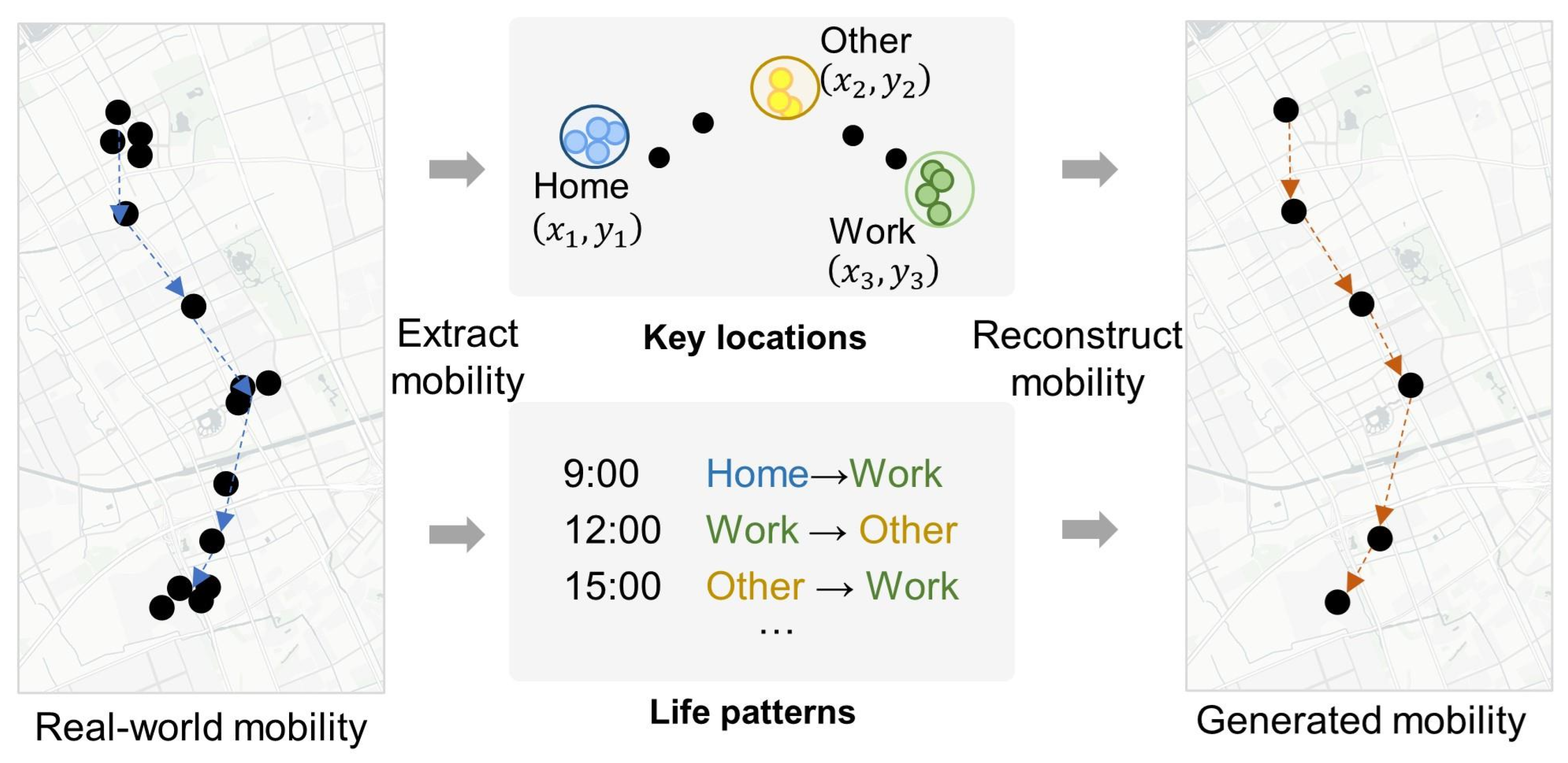
The core premise of the methodology posits that long-term individual mobility information can be effectively represented by a combination of key locations (indicating where an individual participates in various activities) and life patterns (indicating the transitions between these activities).
Key locations are fundamental to understanding individual mobility, acting as pivotal anchor points in daily life. This concept resonates with the “anchor point theory” proposed in 1978, which explains the formation and mechanism of human activity spaces [30]. According to this theory, individuals in unfamiliar environments, such as a new city, initially seek out primary nodes like housing and workplaces—these are their anchor points. Subsequently, secondary nodes and the pathways connecting them, such as the route to work or facilities around the home, are recognized and incorporated into their activity space. This process gradually expands and enriches their activity space, ultimately forming a hierarchical cognitive structure. Key locations, therefore, are not merely isolated points but are central to the formation of an individual’s understanding and navigation of their environment. They define the primary contexts of activities—such as home, work, entertainment, business, etc.—and inherently possess a relational aspect for each individual. For example, u represents the user index, and the identified key locations are , , , representing the key locations for user u.
Life patterns, on the other hand, delve into the fluid nature of daily routines, capturing how individuals transition between key locations over time. These patterns are pivotal in understanding personal mobility, as they encapsulate not just the physical movements but also the underlying behaviors and decisions that guide these movements. Life patterns reflect the intricacies of personal routines, from the choice of routes and the timing of movements to the frequency of visits to certain locations. For instance, the probability of an individual moving from a type A location (e.g., home) to a type B location (e.g., work) at a given time illustrates the predictive aspect of life patterns in daily routines. For instance, m represents the index of the day, and represents the total number of days. indicates the locations of individual u over 24 h on day m. The long-term life pattern of individual u over days is represented as . denotes the long-term life patterns of multiple users.
The combination of key locations and life patterns offers a comprehensive expression of individual long-term travel behavior patterns, encapsulating the essence of personal mobility in urban contexts (see Figure 1). The generation of individual mobility involves extracting key locations and life patterns from the large-scale mobility data of the city, employing mobility generation algorithms, and ultimately generating mobility that does not contain individual private data.

Figure 1.
Concept of mobility generation based on individual key location and life pattern.
For the two scenarios mentioned earlier, we designed a long-term mobility generation algorithm. The model of this study is divided into three modules:
- Module 1, key location and life pattern extraction: Extracting real-world mobility into structured representations of stay points (key locations) and activity patterns (life patterns).
- Module 2, key location and life pattern generation: Generating key locations and life patterns of virtual individuals using a radiation model for key locations and sampling through SVD dimensional reduction for life patterns.
- Module 3, mobility reconstruction: Reconstructing a complete long-term virtual mobility sequence from key locations and life patterns.
The general framework of the model is shown in Figure 2.
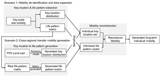
Figure 2.
Methodology framework.
For Scenario 1, the process involves Module 1 + Module 3, where real key locations and life patterns are extracted from real data, then sampled and combined to create virtual mobility data. Key locations, such as work locations, residences, and other places, are extracted from real trajectories. Life patterns represent the transition probabilities between different locations for individuals, also derived from real trajectories. Using these key locations and life patterns, large-scale urban mobility is generated based on the mobility generation algorithm.
As for Scenario 2, the process involves Module 2 + Module 3. Here, new key locations and life patterns for the new city need to be regenerated and then sampled and combined from the generated information to create virtual mobility data. Key locations are estimated using regression models and the radiation model based on POI and other land-use information. New life pattern matrices are generated using the life pattern generation method. Urban mobility patterns are created based on the newly generated key locations and life patterns.
Under this framework, the model structure is flexible and transferable, able to adjust based on the quality of the input data, and has strong interpretability. Combining these three modules allows mobility generation tasks to be effectively accomplished in two different scenarios.
3.2. Key Location Representation and Generation
3.2.1. Extraction and Representation of Key Locations
As defined in the preceding section, key locations serve as the primary anchor points in an individual’s daily life, delineating the primary contexts of activities. In this paper, we define key locations as a combination of home, work, and others. Here, we introduce a rule-based method for identifying an individual’s home, work, and other locations. The identification process follows a well-established approach in the analysis of human mobility data [31,32]. The identification method of home, work, and other is illustrated in Figure 3a, determines these categories based on the duration and timing of the user’s stay at each location. The identification process proceeds as follows:
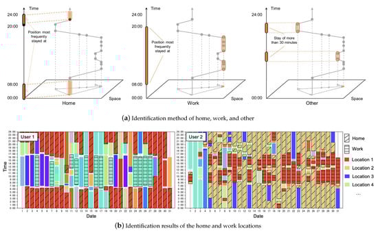
Figure 3.
Identification of key locations.
- Home (H): The location where the user stays nightly (from 20:00 to 08:00 the next morning), on average, exceeds or equals 5 h in 2/3 days during the observation period.
- Work (W): The location where the user stays on average during the daytime (from 08:00 to 20:00) on workdays exceeds 180 min, and the points are not within the residence.
- Other (O): The location where the user stays for more than 30 min, apart from the user’s home and workplace.
For example, in Figure 3b, the identification results of the home and work locations of two mobile phone users are displayed based on their activities over a one-month period, with each distinct color representing a unique location. It should be noted that this framework also accommodates scenarios in which there may be multiple locations for residence, work, and other areas. In the algorithm testing phase of this study, we maintain that users may have up to 5 home locations, 5 work locations, and 10 other locations. When there is more demand, the types and number of key locations can be expanded further.
The home and workplace identification algorithm is provided in the TransBigData Python package [33].
3.2.2. Key Locations Generation
In the task of mobility generation, each generated individual can sample its key locations at home, work, and other sites from this distribution.
Key location information involves the single probability and joint probability distributions of home, work, and other locations. These probabilities can be estimated from transportation surveys, Points of Interest (POIs), land use, road networks, traffic line networks, and other infrastructure and thermal data. The quality of key location estimates varies with the underlying datasets used.
In this study, the generation of key locations is divided into two steps:
Single distribution probability generation: A regression method is used to estimate the single distribution probability of being at home, work, or other. By analyzing basic data such as the POI and thermal data in city grids, the distribution of home, work, and other locations is estimated through a regression model.
Joint distribution probability generation: The joint probability distribution of home, work, and other combinations is generated using a radiation model. This involves estimating the pairwise joint distribution among home, work, and other locations through the radiation model, thereby deducing the overall joint distribution from the individual distributions of HW, HO, and WO.
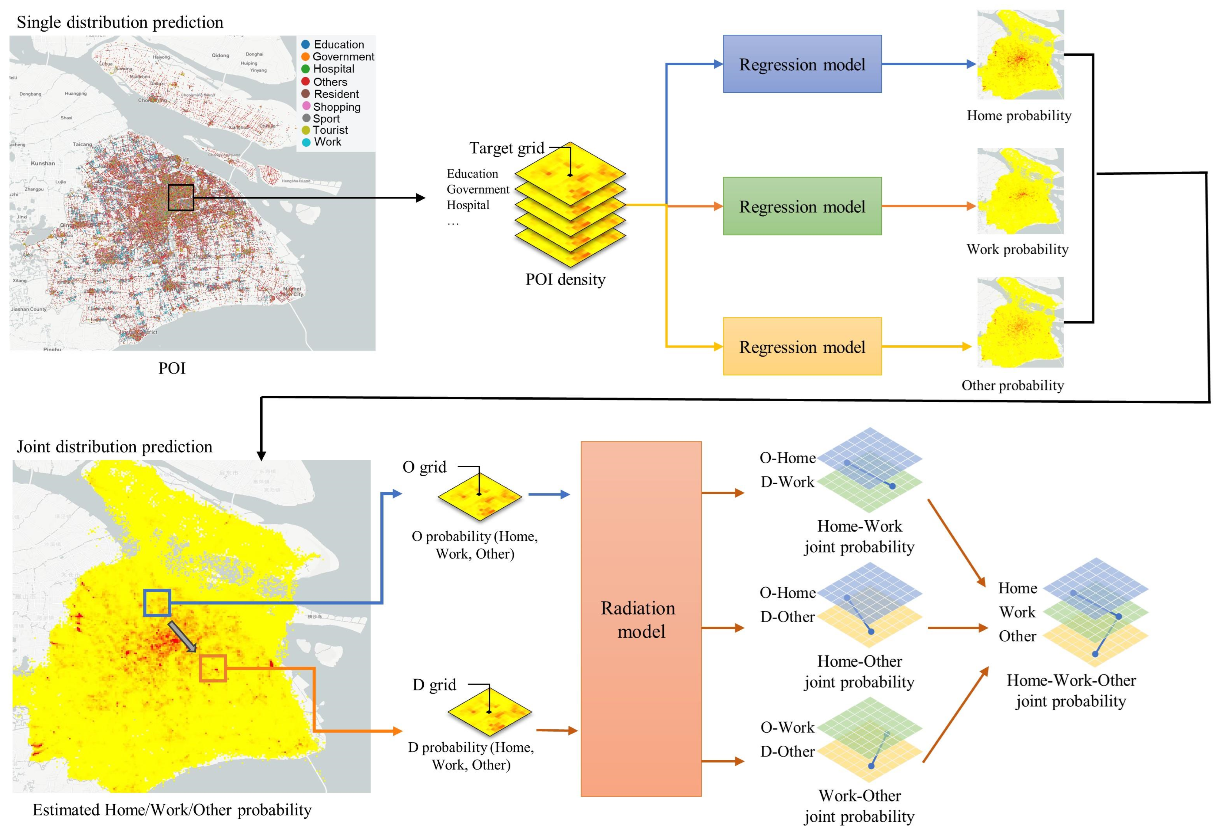
The general method is shown in Figure 4.
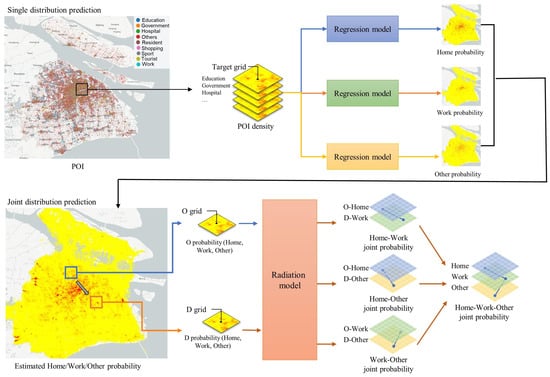
Figure 4.
Distribution estimation of key locations based on radiation model.
To estimate the probability of a single distribution for home, work, and others in a given location, let X denote a characteristic feature vector (e.g., Points of Interest (POIs), population density, land use, and road networks) at this location. The functions , , and represent the probabilities that a grid i is classified as home, work, and other locations, respectively. The regression model can be expressed as:
Here, , , and are regression model functions, and , , and are model parameters. Through this approach, we can predict the likelihood that any location is a residence, workplace, or other location based on basic urban data.
For joint distribution probability generation, a radiation model is established for estimation. The radiation model serves as a mathematical framework for predicting population mobility, commuting patterns, and traffic flow (referenced in a Nature paper). The model is based on the stochastic decision-making process of individuals moving between different locations, considering factors such as population distribution, job opportunities, and distances involved. The core equations of the model are as follows:
Among them, represents the number of people in position i who need to go out to work, which can be expressed as
In Equation (4), represents the commute flow from the home location i to the work location j, respectively, and represents the total number of employment opportunities within a circular area with radius centered at i, excluding the opportunity at i and j.
In the radiation model, indicates the total population within the circular region between grids i and j, with a radius of , excluding the opportunity at the source i and the destination j. This term represents the potential employment opportunities available within a certain distance from the source location i, which is assumed to affect commuting flow .
The radiation model’s fundamental concept lies in considering the employment opportunities in the surrounding areas by individuals when choosing commuting destinations. The model assumes that the number of employment opportunities in each location is proportional to the resident population. Individuals search for job opportunities from all locations, including their own, and select the nearest location that offers better prospects. In this context, “better” refers to job opportunities with attractiveness or benefits that surpass the best opportunity available in the individual’s current location.
As we obtain , we can further estimate the joint probability, which can be represented as:
Similarly, and can be estimated by the same structure.
Furthermore, we can proceed to estimate the joint probability distribution of home, work, and others:
This equation represents the probability that the home location i, the work location j, and the other location k occur simultaneously, given the population distribution and employment opportunities.
Using this approach, we can estimate the joint distribution of key locations in a new area, and then sample based on this distribution to generate the key location combinations for each generated individual.
3.3. Life Pattern Representation and Generation
3.3.1. Extraction and Representation of Life Pattern
Life patterns can be conceptualized through various methodologies, such as matrix representations, where the probabilities of transitioning between locations are quantified; temporal networks, which emphasize the timing and sequence of movements; or even more abstract models that capture the essence of mobility patterns through statistical or machine learning techniques. Each of these approaches offers unique insights into the structure and dynamics of life patterns, highlighting different aspects of how individuals navigate their environments.
This paper adopts a probability-based approach to address the challenge of handling large datasets. It involves analyzing the location data of each user during different time intervals to calculate the transition probabilities between various locations, thereby characterizing the life pattern of each user.
Specifically, the day of a user is divided into multiple time intervals, each with a duration of , such as hours or half-hours. By examining the user’s location information during these intervals and calculating the transition probabilities between different locations, the following expression can be formulated:
Here, represents the number of times user u transitions from location type l to location type k within time window t on a day of type d (for example, weekday and weekend).
Therefore, the life pattern of an individual u can be represented as a vector as:
After acquiring the vector for each user, we can combine all user vectors to create a matrix of life patterns that illustrates the life patterns of all users. If there are n users and each user’s life pattern vector comprises m transition probabilities, the size of the LP matrix would be , with each row denoting a user’s lifestyle pattern vector. The mathematical representation can be depicted as:
Through the matrix, we have recorded the long-term activity pattern information of all individuals in the city.
3.3.2. Matrix Decomposition-Based Life Pattern Generation
When we need to generate individuals, we only need to generate the lifestyle pattern vector of individuals according to the pattern of the LP matrix. However, in practical applications, this matrix is usually very sparse. For example, the life pattern matrix extracted from real mobile phone data consists of 100,000 rows and 3034 columns, where the 100,000 rows represent individual users and the 3034 columns represent transition probabilities. Notably, only 5.33% of the values in this matrix are non-zero. We can use matrix-dimensionality reduction methods such as SVD, NMF, etc., to extract patterns and generate individuals based on these patterns. For example, here, we use the SVD method for decomposition. Performing SVD decomposition on the LP matrix can be represented as follows:
The matrix can be decomposed into three main components: two orthogonal matrices U and V, along with a diagonal matrix . The elements on the diagonal of the matrix are singular values , arranged in descending order. These singular values reflect the importance or “strength” of different patterns in the data. The matrix U and the matrix V represent the “patterns” in the user and the transition mode, respectively.
In this decomposition, each term represents a major pattern in the matrix , where is the directional vector of that pattern in the user lifestyle space, and is the directional vector of that pattern in the space of transition mode. The singular value indicates the importance or contribution of that pattern. By selecting the first few largest singular values and their corresponding and , we can approximate the reconstruction of the LP matrix, capturing the most important patterns in the data while eliminating noise and unimportant details.
represents the basis for individual lifestyle patterns in the original data. These bases can be seen as the “components” that make up all individual lifestyle patterns. When generating new individuals, it is possible to keep the V matrix and the matrix unchanged and use the existing lifestyle pattern bases (i.e., vectors in ) to construct or generate the lifestyle patterns of new individuals.
The key to this method is that by adjusting the values in the matrix U, we can generate new individuals with specific characteristics of the lifestyle pattern. By changing the values in U, we can adjust the composition of the lifestyle patterns of new individuals and generate lifestyle patterns with different characteristics. Specifically, when generating new individuals, a new matrix U can be created as . The matrix can be determined by random generation or specific rules, where each row represents the strength of association between a new individual and each base vector in .
Here, we assume that each column of the matrix U follows a normal distribution. By extracting the parameters of the normal distribution for each column (i.e., mean and standard deviation), we can use these parameters to generate a new matrix and subsequently create new individual lifestyle pattern vectors. The following are the specific steps and formulas:
1. Extract distribution parameters of columns in matrix U: For each column c in the matrix U, calculate the mean and the standard deviation of that column. This can be performed using the following formulas:
Here, represents the element in the i-th row and c-th column of matrix U, and n is the number of rows in matrix U (i.e., the number of users).
2. Generate a new matrix : Using the mean and standard deviation calculated for each column in Step 1, for each column in the new matrix , we can randomly generate new elements from a normal distribution. Specifically, for each element in , it can be generated using the following formula:
Here, denotes a normal distribution with mean and variance .
Following the above steps, we can generate a new matrix containing new elements generated based on the distribution of the original columns in the matrix U. This approach allows us to generate new individuals with similar distribution characteristics while preserving the original distribution of lifestyle patterns. The newly generated matrix can be combined with the original matrices V and to generate new individual lifestyle patterns using the following formula:
3.4. Generation of Long-Term Individual Mobility from Key Location and Life Pattern
Reconstructing an individual’s mobility from the life pattern vector involves two key elements: (1) transition probabilities between stay points, and (2) duration of stay at each stay point. In this model, the transition probability from one stay point to another is modeled using a Markov chain-based model, while the duration of staying in a state is determined by the Gaussian Mixture probability distribution (GMM) fitted based on individual data statistics.
Here, the mobility generation model uses a Markov chain model to generate life pattern sequences, thereby simulating users’ life patterns. The Markov chain model assumes that the next state of a system depends only on the current state and is independent of previous states [34]. This assumption simplifies the modeling process of complex systems, making the model easier to understand and implement. In relevant studies, the Markov chain model is widely used to simulate and predict individual travel behaviors [35,36,37,38].
The individual life pattern vector that was extracted earlier actually records the probabilities of a user moving from one location to another at different time periods, which corresponds to the transition probability matrix in the Markov chain model.
For a user u where his or her home, work, and other location is
which presents all key locations of the user u.
For the user states represented as with length m, the state transition matrix of the individual u at time t on day d is
where the transition probability is calculated by vector :
Next, an algorithm is designed to construct individual long-term mobility mobility based on life pattern sequences and key locations.
In the algorithm, distinct transition matrices are applied for commute and non-commute days for each individual. Initially, the algorithm initializes the initial state, including activity type and geographic coordinates. Subsequently, guided by the state transition probability matrix , the model determines the next state of the user, distinguishing between locations such as work, home, or other places. Following this, the model computes the duration of each state based on its type, determining the start and end hours of activities, and adding a random time deviation within [−30, 30] minutes to adjust the start and end times to the minute level. These durations are then incorporated into the sequence of activity patterns. This iterative process continues until the generated mobility sequence reaches the specified period. Ultimately, this results in an individual’s travel chain, encompassing activity types, durations, and geographic positions selected from , thus capturing the individual’s mobility pattern comprehensively. The overall process of the algorithm is depicted in Algorithm 1.
| Algorithm 1 Generate long-term mobility |
|
4. Case Study and Result
4.1. Data and Study Area
For the research, anonymous data from mobile phone data from Shanghai and Beijing were used for testing. The mobile signaling data used in this study were obtained from mobile operators and originally gathered for billing and operational purposes. The Shanghai dataset comprises information from over 27 million users with a daily volume of approximately 80 million records, covering the period from 13 to 19 November 2023. From these 27 million users, we randomly selected two groups of 30,000 regular users (those who stayed more than two-thirds of the days in a month) for comparative validation in our results. The Beijing dataset includes data of similar quality from November 2023. Each data record includes various information, such as an encrypted user ID number, the timestamp of the signal event, and the user’s location coordinates. The user’s location coordinates were obtained from the latitude and longitude of the nearest connected base station to the user.
4.2. Results
4.2.1. Mobility Generation from Individual- to City-Scale Dynamic
In this experiment, the model we propose was applied to generate the mobility patterns of 30,000 virtual users over 7 days in Shanghai; the key location and the life pattern information were sampled from the result identified and extracted from real-world mobility data. The specific format of the generated mobility dataset is presented in Table 1, which details the specifics of each data entry corresponding to the visit of a user to a particular location.

Table 1.
Example of generated mobility.
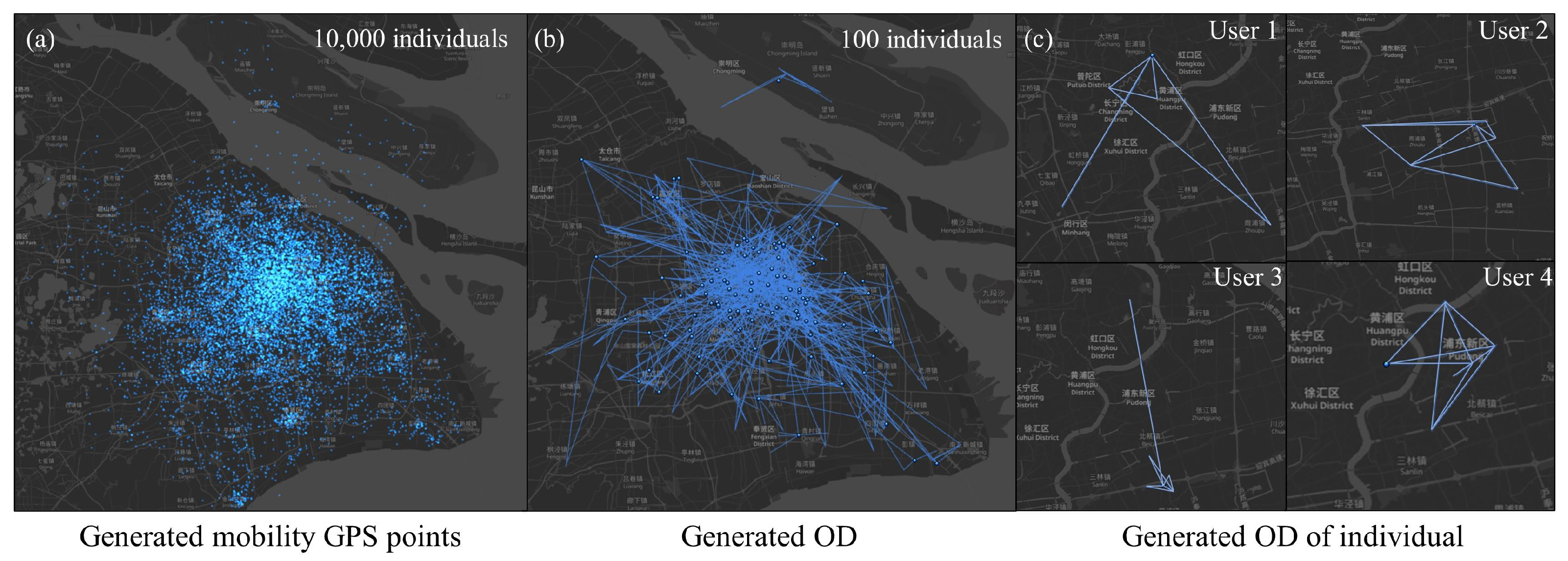
Figure 5 provides a comprehensive visualization of the generated mobility results, offering insights into individual and collective mobility patterns within an urban context.

Figure 5.
Result of generated mobility.
Figure 5a presents the GPS location distribution for a subset of 10,000 users, providing a snapshot of spatial activity and highlighting high-density areas that often correspond to residential, commercial, or industrial zones. This spatial distribution is crucial for understanding the geographical spread of activities and the interaction of individuals with the urban environment. Figure 5b focuses on the OD patterns of travel of 100 users during the same seven-day period, illustrating the diversity of travel behaviors between individuals. This component of the analysis reveals the complexity of urban mobility, with each individual’s movements weaving a unique narrative of daily life and interactions with the city. Figure 5c selects and details the seven-day OD distribution for four individuals, showcasing the variability of life patterns between residents. The OD mappings form polygonal shapes, representing each individual’s activity space, encompassing the residential, workplace and other locations frequented. This polygonal representation is a graphical embodiment of the concept of a life pattern, highlighting the regularity and predictability of individual mobility within the urban tapestry.
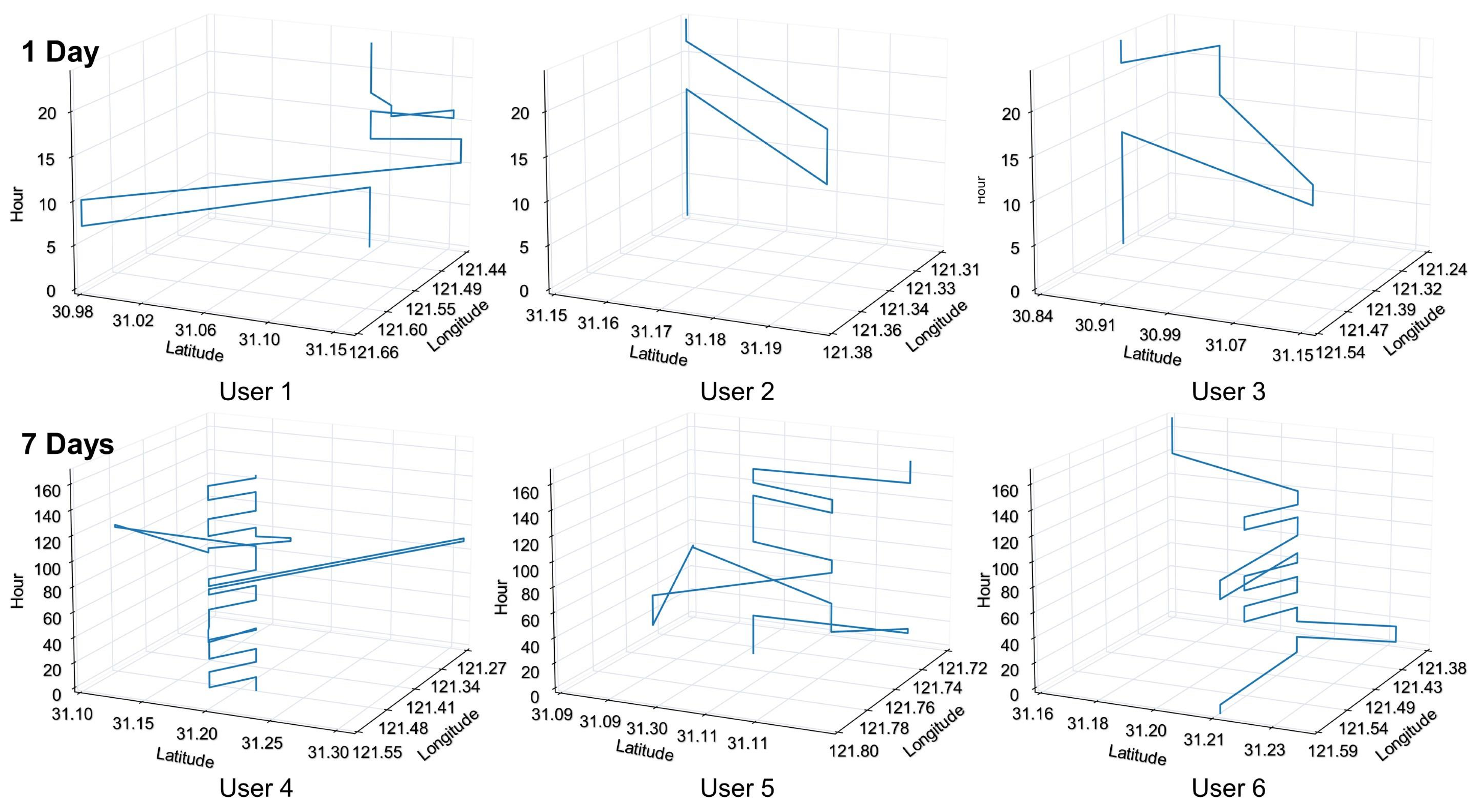
From a micro-perspective, the generated results encapsulate distinct life patterns, with individuals routinely moving between their homes, workplaces, and other destinations in a manner that reflects their personal routines and preferences, as shown in Figure 6. These life patterns, manifested through the OD polygons, delineate each individual’s activity space, offering a visual representation of their daily interactions with the city. On a macro-scale, the aggregate data from all generated mobility align closely with the actual urban activity patterns observed in Shanghai. The data show a concentration of activities in the city center with a dispersal into the suburbs, mirroring the real-life dynamics of urban sprawl and centralization. This congruence between the generated mobility patterns and real-world observations validates the effectiveness of our model in capturing the essence of urban mobility, from the routine movements of individuals to the broader patterns of collective behavior.
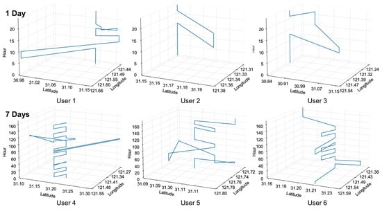
Figure 6.
Example of generated spatial–temporal mobility.
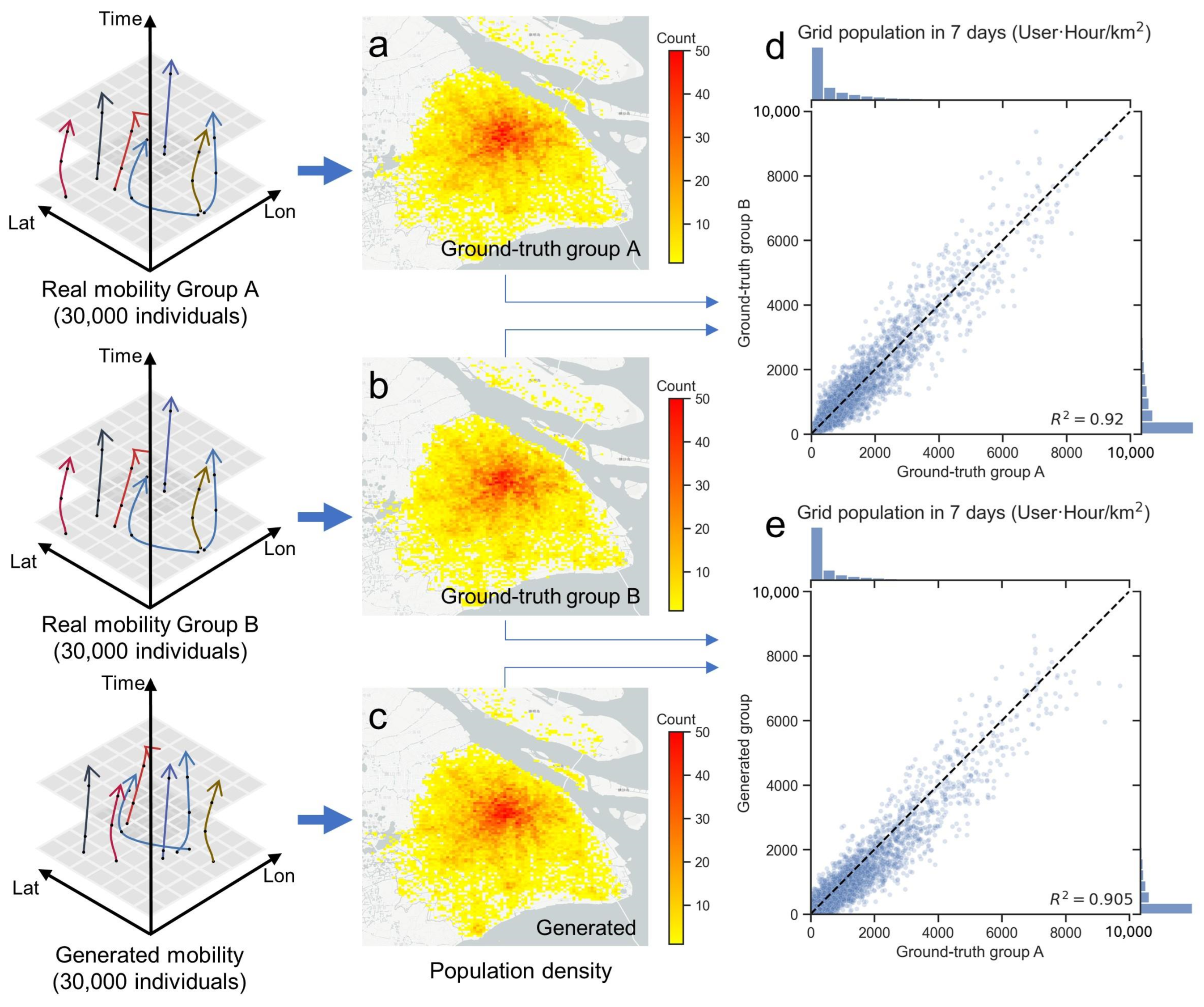
To assess the precision and realism of the synthetic mobility generated by our framework, we conducted a detailed comparison with actual mobility data. This involved aggregating the generated mobility data into 1 km × 1 km grid cells and then comparing the population densities within these cells. The population density was derived from mobility data, aggregating the number of people within each grid at a specific time. The grid-level population density was compared on an hourly basis over a period of 7 days. However, it is essential to acknowledge the presence of natural fluctuations in real-world mobility data. For example, sampling 30,000 individuals and their activities in a specific grid cell will not yield exactly the same numbers if a different set of 30,000 individuals were sampled, due to the inherent variability in human movement patterns. Recognizing this, the closer the generated data align with these natural fluctuations, the more accurately they can be said to reflect real-world conditions.
To facilitate a fair comparison under the same criteria, we virtually sampled 30,000 users (generated group) and conducted two random samplings of 30,000 users each from the actual mobility data (ground-truth group A and ground-truth group B). By aggregating these samples into grid cells, we could directly compare the results.
Figure 7a–c display the population density calculated from real data group A (Figure 7a), real data group B (Figure 7b), and the generated data group (Figure 7c), respectively. Figure 7d compares ground-truth group A with ground-truth group B, showing a value of 0.92. The scatterplot in Figure 7e illustrates the comparison of 24 h grid heatmaps between the generated group and ground-truth group A, with each point representing the population count of a grid at a specific time. The general high correlation ( = 0.905) indicates a strong similarity between the generated and ground-truth data. The distribution of points suggests that the population heatmap generated by our model closely mirrors the actual population, demonstrating the effectiveness of our approach in replicating real-world population distributions within urban grids.
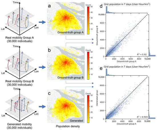
Figure 7.
Comparison of generated mobility on grid-level population aggregate.
4.2.2. Transferability of Individual’s Life Pattern
In order to test the transferability of the individual life pattern proposed in this study, several experiments were conducted.
To examine the transferability of life patterns within different areas of the same city, a test was carried out by dividing Shanghai into two regions: Pudong and Puxi.
We tested scenarios where the life pattern from Puxi was combined with key locations in Pudong to generate virtual mobility, as well as scenarios where Puxi’s life pattern was combined with key locations across the entire city of Shanghai. Similarly, we tested the life pattern from Pudong combined with key locations throughout Shanghai and finally a scenario using Shanghai’s overall life pattern with citywide key locations.
In addition, we conducted experiments on the transferability of life patterns between different cities. We extracted the life pattern information of 100,000 individuals from a dataset in Beijing and combined these with key locations in Shanghai to generate 30,000 virtual mobility. Then, these were compared against an actual set of 30,000 mobility to evaluate the performance.
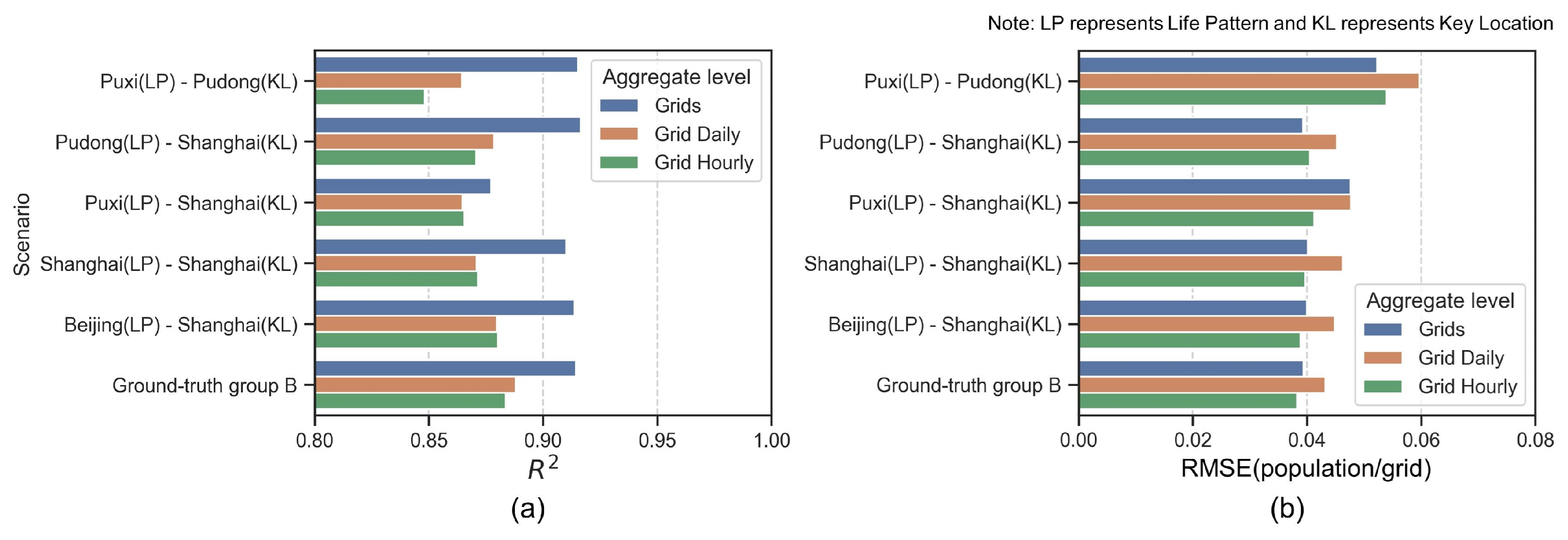
Figure 8a,b represent the results of experiments conducted to test the transferability of individual life patterns in different scenarios using metrics (Figure 8a) and the Root Mean Square Error (RMSE) (Figure 8b), respectively.
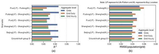
Figure 8.
Performance of generated mobility (population density comparing with ground-truth group A).
All scenarios show relatively high values, above 0.80, indicating good model performance in different setups. The consistency across scenarios suggests that the model effectively captures the essential characteristics of life patterns for both intracity (Shanghai) and intercity (Beijing to Shanghai) transfers. RMSE values are relatively low across all scenarios, with the highest value around 0.04, which is still quite low, indicating minor prediction errors. The “ground-truth group B” serves as a benchmark or control group, showing how well the model performs relative to actual data.
The experiments demonstrate that the life patterns derived from one part of a city (e.g., Puxi) can effectively be transferred to predict behaviors in another part of the same city (e.g., Pudong) or even across cities (e.g., from Beijing to Shanghai). The models exhibit robustness and reliability in using life patterns and key locations to generate virtual mobility that closely mirrors the actual patterns observed in the data. This suggests a strong potential for using these models in urban planning, traffic management, and similar applications where understanding and predicting human mobility patterns is crucial.
4.2.3. Representative Performance of Generated Mobility
Generating precise individual mobility is a time- and computation-power-consuming process. Therefore, it is necessary to reduce the number of individuals generated while maintaining its ability to depict the mobility pattern in a city. For this purpose, a series of experiments were conducted to investigate the adequacy of generated individual mobility in representing the overall urban mobility patterns.
The experiments involved setting the range of synthetic individual mobility from 0 to 100,000, sampled at intervals of 1000 individuals. The individual mobility produced was then aggregated at a spatial resolution of 1 km × 1 km grid scale, with hourly and daily temporal resolutions. The aggregated results were then compared with the population density aggregated at the same scale of real mobile phone signal data representing 8.08 million users. To ensure the consistency and comparability of statistical data, both sets of data were normalized to a range of 0–1, eliminating differences in magnitudes that may exist between different datasets and ensuring the precision of the data analysis.
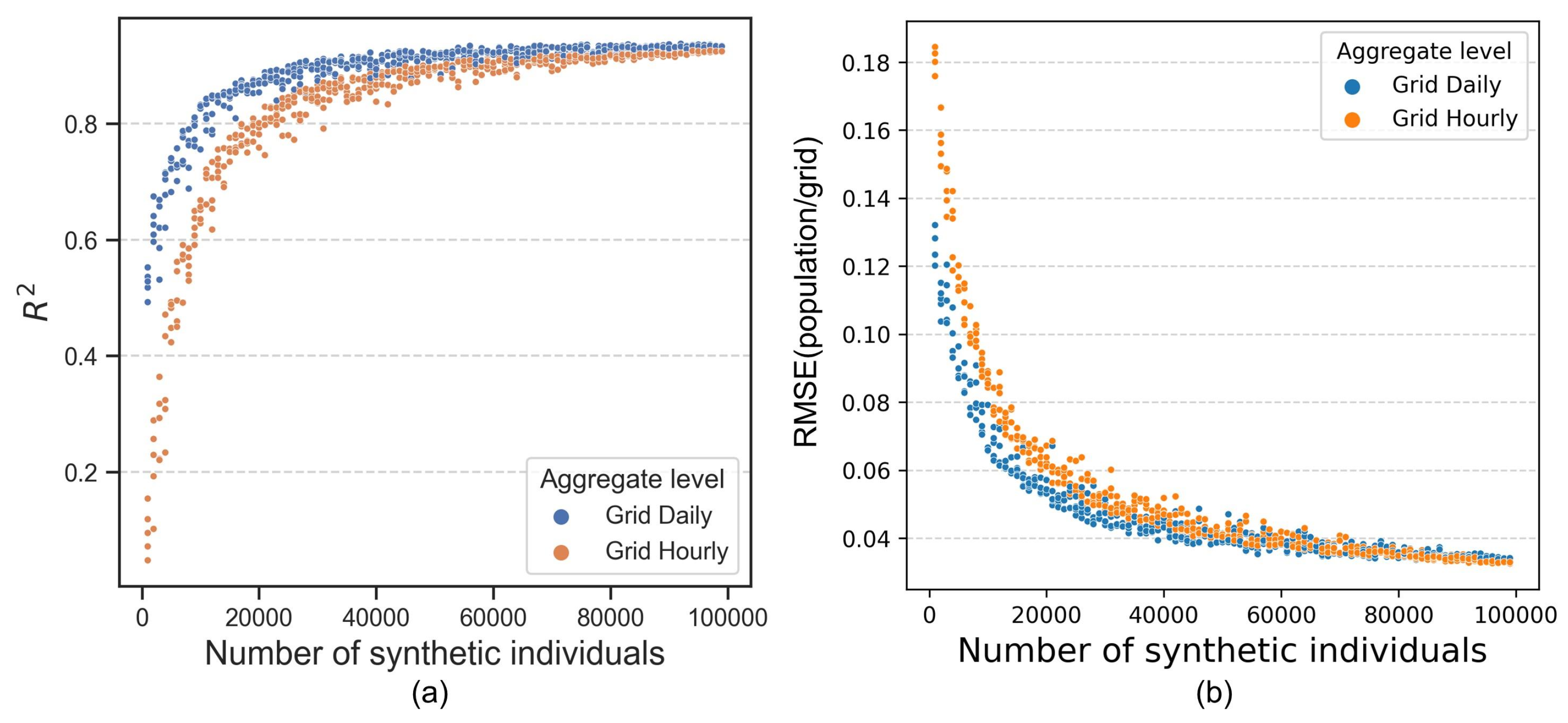
Figure 9 illustrates the relationship between the number of synthetic individuals and its representative performance described by two statistical metrics of (Figure 9a) and RMSE (Figure 9b) compared to the density of the real population. Illustrated in both figures, as the number of synthetic individuals increases, the aggregated daily and hourly results show a tendency to stabilize, with the daily performance generally exceeding that of the hourly performance. When the results of the virtual individual generated reach around 10,000, the generated mobility can describe the population dynamics at the city level with an of over 0.8 for daily granularity and requires over 20,000 individuals for hourly granularity. In fact, this result also demonstrates that the use of only about 0.25% of the sampled individuals (20,000 out of 8.08 million) is sufficient to represent the dynamic changes of the entire urban population, further proving the value of mobility generation technology in this study.
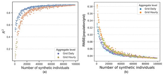
Figure 9.
Representative performance of generated mobility comparing with real population density.
5. Conclusions
This study has developed and implemented a novel GIS-based framework for generating city-scale individual-level spatio-temporal mobility patterns. By integrating the concept of key locations with dynamic life patterns, we have proposed a comprehensive approach to model and simulate the complex movements of individuals within urban environments. The main conclusions are as follows.
- Taking real long-term mobility data from Shanghai to extract the life patterns and key locations, the proposed methodology was successfully applied to generate the mobility of 30,000 virtual users over 7 days in Shanghai.
- By testing the combination of key locations and life patterns extracted from real-world mobility data in different areas, the model demonstrated strong transferability between various areas within cities and across different cities.
- By testing the representatives of the generated mobility data, we found that using only about 0.25% of the generated individuals’ mobility is sufficient to represent the dynamic changes of the entire urban population in daily and hourly resolution, at a 1 km × 1 km grid level, compared to real-world mobility datasets.
This study provides a new method to generate long-term spatiotemporal mobility patterns at the individual level, offering valuable tools for city managers, planners, and policymakers to address the growing challenges of transportation in the urbanization process. Real-world mobility data contain specific user travel patterns, work locations, home addresses, and daily activity locations, which involve privacy and sensitive information. This makes the widespread use of real-world mobility data in urban planning and management a challenge, limiting the intelligent management and sustainable development of cities. Therefore, this study proposes an individual mobility generation method based on key locations and life patterns, effectively enhancing the applicability of mobility for broader use and providing support for urban planning. Additionally, by constructing key urban information, this research generates large-scale urban travel mobility, transforming limited mobility data into comprehensive city-wide travel patterns. This provides a foundation for large-scale urban mobility analysis.
Author Contributions
Conceptualization, Yao Yao, Yinghong Jiang and Qing Yu; methodology, Yao Yao and Qing Yu; software, Yao Yao and Qing Yu; validation, Yao Yao and Qing Yu; formal analysis, Yao Yao, Jian Yuan, and Qing Yu; data curation, Jian Xu; writing—original draft preparation, Yao Yao, Jiaxing Li and Jian Xu; writing—review and editing, Yao Yao, Siyuan Liu and Qing Yu; visualization, Qing Yu; supervision, Haoran Zhang. All authors have read and agreed to the published version of the manuscript.
Funding
This work was supported by Shanghai Super Postdoctoral Funding Project (No.2023045) and Key Laboratory of Road and Traffic Engineering of the Ministry of Education, Tongji University (No. K202301).
Data Availability Statement
Data available on request due to restrictions.
Acknowledgments
The author would like to thank the anonymous reviewers for their comments.
Conflicts of Interest
Authors Yao Yao and Yinghong Jiang are employed by the company Shanghai Urban Construction Design and Research Institute (Group) Co., Ltd. The remaining authors declare that the research was conducted in the absence of any commercial or financial relationships that could be construed as a potential conflict of interest.
References
- Forghani, M.; Karimipour, F.; Claramunt, C. From cellular positioning data to trajectories: Steps towards a more accurate mobility exploration. Transp. Res. Part C Emerg. Technol. 2020, 117, 102666. [Google Scholar] [CrossRef]
- Fekih, M.; Bellemans, T.; Smoreda, Z.; Bonnel, P.; Furno, A.; Galland, S. A data-driven approach for origin–destination matrix construction from cellular network signalling data: A case study of Lyon region (France). Transportation 2021, 48, 1671–1702. [Google Scholar] [CrossRef]
- Ghahramani, M.; Zhou, M.; Wang, G. Urban sensing based on mobile phone data: Approaches, applications, and challenges. IEEE/CAA J. Autom. Sin. 2020, 7, 627–637. [Google Scholar] [CrossRef]
- Yang, M.; Luo, W.; Ashoori, M.; Mahmoudi, J.; Xiong, C.; Lu, J.; Zhao, G.; Saleh Namadi, S.; Hu, S.; Kabiri, A.; et al. Big-data driven framework to estimate vehicle volume based on mobile device location data. Transp. Res. Rec. 2024, 2678, 352–365. [Google Scholar] [CrossRef]
- Liu, Y.; Fang, F.; Jing, Y. How urban land use influences commuting flows in Wuhan, Central China: A mobile phone signaling data perspective. Sustain. Cities Soc. 2020, 53, 101914. [Google Scholar] [CrossRef]
- Harrison, G.; Grant-Muller, S.M.; Hodgson, F.C. New and emerging data forms in transportation planning and policy: Opportunities and challenges for “Track and Trace” data. Transp. Res. Part C Emerg. Technol. 2020, 117, 102672. [Google Scholar] [CrossRef]
- Ismagilova, E.; Hughes, L.; Rana, N.P.; Dwivedi, Y.K. Security, privacy and risks within smart cities: Literature review and development of a smart city interaction framework. Inf. Syst. Front. 2022, 24, 393–414. [Google Scholar] [CrossRef] [PubMed]
- Savage, N. Synthetic data could be better than real data. Nature, 2023; Online ahead of print. [Google Scholar]
- Yin, B.; Leurent, F. What are the multimodal patterns of individual mobility at the day level in the Paris region? A two-stage data-driven approach based on the 2018 Household Travel Survey. Transportation 2023, 50, 1497–1526. [Google Scholar] [CrossRef]
- Huang, Y.; Gao, L.; Ni, A.; Liu, X. Analysis of travel mode choice and trip chain pattern relationships based on multi-day GPS data: A case study in Shanghai, China. J. Transp. Geogr. 2021, 93, 103070. [Google Scholar] [CrossRef]
- Cao, J.; Li, Q.; Tu, W.; Gao, Q.; Cao, R.; Zhong, C. Resolving urban mobility networks from individual travel graphs using massive-scale mobile phone tracking data. Cities 2021, 110, 103077. [Google Scholar] [CrossRef]
- Lidbe, A.; Adanu, E.K.; Penmetsa, P.; Jones, S. Changes in the travel patterns of older Americans with medical conditions: A comparison of 2001 and 2017 NHTS data. Transp. Res. Interdiscip. Perspect. 2021, 11, 100463. [Google Scholar] [CrossRef]
- Wang, S.; Mei, G.; Cuomo, S. A generic paradigm for mining human mobility patterns based on the GPS trajectory data using complex network analysis. Concurr. Comput. 2021, 33, e5335. [Google Scholar] [CrossRef]
- Jiang, B.; Yin, J.; Zhao, S. Characterizing the human mobility pattern in a large street network. Phys. Rev. E Stat. Nonlinear Soft Matter Phys. 2009, 80, 021136. [Google Scholar] [CrossRef]
- González, M.C.; Hidalgo, C.A.; Barabási, A.L. Understanding individual human mobility patterns. Nature 2009, 458, 238. [Google Scholar] [CrossRef]
- Kung, K.S.; Greco, K.; Sobolevsky, S.; Ratti, C. Exploring universal patterns in human home-work commuting from mobile phone data. PLoS ONE 2014, 9, e96180. [Google Scholar] [CrossRef]
- Arcolezi, H.H.; Couchot, J.F.; Renaud, D.; Al Bouna, B.; Xiao, X. Differentially private multivariate time series forecasting of aggregated human mobility with deep learning: Input or gradient perturbation? Neural Comput. Appl. 2022, 34, 13355–13369. [Google Scholar] [CrossRef]
- Wang, Y.; Currim, F.; Ram, S. Deep Learning of Spatiotemporal Patterns for Urban Mobility Prediction Using Big Data. Inf. Syst. Res. 2022, 33, 579–598. [Google Scholar] [CrossRef]
- Yang, D.; Fankhauser, B.; Rosso, P.; Cudre-Mauroux, P. Location prediction over sparse user mobility traces using rnns. In Proceedings of the Twenty-Ninth International Joint Conference on Artificial Intelligence, Yokohama, Japan, 11–17 July 2020; pp. 2184–2190. [Google Scholar]
- Deng, B.; Yang, D.; Qu, B.; Fankhauser, B.; Cudre-Mauroux, P. Robust Location Prediction over Sparse Spatiotemporal Trajectory Data: Flashback to the Right Moment. ACM Trans. Intell. Syst. Technol. 2023, 14, 1–24. [Google Scholar] [CrossRef]
- Abideen, Z.U.; Sun, H.; Yang, Z.; Ahmad, R.Z.; Iftekhar, A.; Ali, A. Deep Wide Spatial-Temporal Based Transformer Networks Modeling for the Next Destination According to the Taxi Driver Behavior Prediction. Appl. Sci. 2021, 11, 17. [Google Scholar] [CrossRef]
- Chen, Y.; Long, C.; Cong, G.; Li, C. Context-aware Deep Model for Joint Mobility and Time Prediction. In Proceedings of the WSDM ’20: The Thirteenth ACM International Conference on Web Search and Data Mining, Houston, TX, USA, 3–7 February 2020. [Google Scholar]
- Celes, C.; Boukerche, A.; Loureiro, A.A.F. Generating and Analyzing Mobility Traces for Bus-Based Vehicular Networks. IEEE Trans. Veh. Technol. 2023, 72, 16409–16425. [Google Scholar] [CrossRef]
- Song, H.Y.; Baek, M.S.; Sung, M. Generating Human Mobility Route Based on Generative Adversarial Network. In Proceedings of the 2019 Federated Conference on Computer Science and Information Systems (FedCSIS), Leipzig, Germany, 1–4 September 2019; pp. 91–99. [Google Scholar]
- Memon, I.; Chen, L.; Majid, A.; Lv, M.; Hussain, I.; Chen, G. Travel Recommendation Using Geo-tagged Photos in Social Media for Tourist. Wirel. Pers. Commun. 2015, 80, 1347–1362. [Google Scholar] [CrossRef]
- Song, C.; Koren, T.; Wang, P.; Barabási, A.L. Modelling the scaling properties of human mobility. Nat. Phys. 2010, 6, 818–823. [Google Scholar] [CrossRef]
- Cao, C.; Li, M. Generating Mobility Trajectories with Retained Data Utility. In Proceedings of the KDD ’21: The 27th ACM SIGKDD Conference on Knowledge Discovery and Data Mining, Singapore, 14–18 August 2021. [Google Scholar]
- Long, Q.; Wang, H.; Li, T.; Huang, L.; Wang, K.; Wu, Q.; Li, G.; Liang, Y.; Yu, L.; Li, Y. Practical Synthetic Human Trajectories Generation Based on Variational Point Processes. In Proceedings of the 29th ACM SIGKDD Conference on Knowledge Discovery and Data Mining, KDD ’23, New York, NY, USA, 6–10 August 2023; pp. 4561–4571. [Google Scholar] [CrossRef]
- Zhu, Y.; Ye, Y.; Zhao, X.; Yu, J.J. Diffusion model for GPS trajectory generation. arXiv 2023, arXiv:2304.11582. [Google Scholar]
- Golledge, R.G. Learning about urban environment. In Timing Space and Spacing Time Vol. 1: Making Sense of Time; Edward Arnold: London, UK, 1978; pp. 76–98. [Google Scholar]
- Li, W.; Cheng, X.; Duan, Z.; Yang, D.; Guo, G. A framework for spatial interaction analysis based on large-scale mobile phone data. Comput. Intell. Neurosci. 2014, 2014, 21. [Google Scholar] [CrossRef]
- Yu, Q.; Li, W.; Yang, D.; Zhang, H. Mobile phone data in urban commuting: A network community detection-based framework to unveil the spatial structure of commuting demand. J. Adv. Transp. 2020, 2020, 1–15. [Google Scholar] [CrossRef]
- Yu, Q.; Yuan, J. TransBigData: A Python package for transportation spatio-temporal big data processing, analysis and visualization. J. Open Source Softw. 2022, 7, 4021. [Google Scholar] [CrossRef]
- Norris, J.R. Markov Chains; Number 2; Cambridge University Press: Cambridge, UK, 1998. [Google Scholar]
- Huang, W.; Li, S.; Liu, X.; Ban, Y. Predicting human mobility with activity changes. Int. J. Geogr. Inf. Sci. 2015, 29, 1569–1587. [Google Scholar] [CrossRef]
- Jiang, J.; Pan, C.; Liu, H.; Yang, G. Predicting human mobility based on location data modeled by Markov chains. In Proceedings of the 2016 Fourth International Conference on Ubiquitous Positioning, Indoor Navigation and Location Based Services (UPINLBS), Shanghai, China, 2–4 November 2016; pp. 145–151. [Google Scholar]
- Lv, Q.; Qiao, Y.; Ansari, N.; Liu, J.; Yang, J. Big data driven hidden Markov model based individual mobility prediction at points of interest. IEEE Trans. Veh. Technol. 2016, 66, 5204–5216. [Google Scholar] [CrossRef]
- Saadi, I.; Mustafa, A.; Teller, J.; Cools, M. Forecasting travel behavior using Markov Chains-based approaches. Transp. Res. Part C Emerg. Technol. 2016, 69, 402–417. [Google Scholar] [CrossRef]


Disclaimer/Publisher’s Note: The statements, opinions and data contained in all publications are solely those of the individual author(s) and contributor(s) and not of MDPI and/or the editor(s). MDPI and/or the editor(s) disclaim responsibility for any injury to people or property resulting from any ideas, methods, instructions or products referred to in the content. |
© 2024 by the authors. Licensee MDPI, Basel, Switzerland. This article is an open access article distributed under the terms and conditions of the Creative Commons Attribution (CC BY) license (https://creativecommons.org/licenses/by/4.0/).