Abstract
Land use/cover change (LUCC) refers to the phenomenon of changes in the Earth’s surface over time. Accurate prediction of LUCC is crucial for guiding policy formulation and resource management, contributing to the sustainable use of land, and maintaining the health of the Earth’s ecosystems. LUCC is a dynamic geographical process involving complex spatiotemporal dependencies. Existing LUCC simulation models suffer from insufficient spatiotemporal feature learning, and traditional cellular automaton (CA) models exhibit limitations in neighborhood effects. This study proposes a cellular automaton model based on spatiotemporal feature learning and hotspot area pre-allocation (VST-PCA). The model utilizes the video swin transformer to acquire transformation rules, enabling a more accurate capture of the spatiotemporal dependencies inherent in LUCC. Simultaneously, a pre-allocation strategy is introduced in the CA simulation to address the local constraints of neighborhood effects, thereby enhancing the simulation accuracy. Using the Chongqing metropolitan area as the study area, two traditional CA models and two deep learning-based CA models were constructed to validate the performance of the VST-PCA model. Results indicated that the proposed VST-PCA model achieved Kappa and FOM values of 0.8654 and 0.4534, respectively. Compared to other models, Kappa increased by 0.0322–0.1036, and FOM increased by 0.0513–0.1649. This study provides an accurate and effective method for LUCC simulation, offering valuable insights for future research and land management planning.
1. Introduction
Land use/cover change (LUCC) refers to the phenomenon of changes over time in the utilization and coverage of the Earth’s surface. On the one hand, LUCC is influenced by human activities; on the other hand, it directly impacts various aspects such as ecosystem health, carbon sequestration, climate change, and natural disaster prevention [1,2,3,4]. Simulating LUCC allows for a better understanding and prediction of the causes and consequences of these changes, thereby supporting sustainable development and environmental conservation.
The model based on cellular automata (CA) is a widely used approach for simulating LUCC. This model possesses characteristics of discreteness, dynamics, and self-organization, enabling it to effectively simulate the discrete and temporally strong process of land use change [5]. However, traditional CA models have some limitations, primarily manifested in the following aspects: (1) they only consider direct interactions between land use units, overlooking the complex relationships between human activities, policy changes, climate variations, and land use [6], and (2) they are unable to handle highly nonlinear relationships to thoroughly explore transformation rules [7]. In recent years, one focus of research has been on integrating CA models with other modeling methods to construct more applicable hybrid models. Existing studies have mainly concentrated on integrating regression analysis [8], random forest (RF) [9,10,11], support vector machine (SVM) [12], neural networks [13,14], and other machine learning and deep learning methods to capture the influences of changes and external factors as well as to unearth potential land use transition rules [9]. Moreover, the integration of CA models with other geographical mechanistic models (such as ecological models and climate models) to consider broader environmental factors and ecosystem impacts and enhance model interpretability has also become a focus of research [15,16].
In the process of researching LUCC, spatiotemporal factors are fundamental for understanding and predicting the dynamics of LUCC, which is crucial for constructing accurate models. Spatial factors typically include topography (such as slope and elevation), the distribution of water bodies, and the spatial distribution of human activities like urbanization or agricultural expansion. These spatial attributes determine the feasibility and sustainability of land use types within a region, thereby directly influencing the patterns of land use change [17,18]. Temporal factors encompass both long-term and short-term changes, including population shifts, economic development levels, climate change trends, and variations in policies and regulations [19]. Spatial factors provide the physical and geographical conditions for land use changes, while temporal factors reflect the evolution and dynamics of these changes over time [20]. Considering these spatiotemporal factors comprehensively is essential for a deep understanding of the dynamics of land use and its driving mechanisms.
The CA model is primarily composed of four elements: space, cell, neighborhood effect, and transition rules [21]. In CA modeling, a significant amount of research attention has been focused on exploring transition rules and neighborhood effects [22]. In CA models for LUCC simulation, accurately calculated transition rules are a crucial factor determining the predictive capability of the model. These rules determine the likelihood of cells transitioning from one state to another in the simulation. Essentially, these rules represent spatiotemporal transformation patterns governed by the complex relationships and feedback between land use and driving factors. LUCC is a dynamic geographical process involving intricate spatiotemporal dependencies. The conversion of target land units is influenced by both spatial correlations and temporal dependencies. Spatial correlation can be understood as the greater impact of closer grids on the target grid compared to those farther away, while temporal dependency refers to the influence of past attributes on the future land use type [23]. One current academic focus is how to leverage deep learning methods to extract spatiotemporal features [24,25]. In terms of spatial correlation, convolutional neural networks (CNNs) have been proven effective in capturing complex features of driving factors within the neighborhood of each unit in urban expansion simulation [26,27]. In the study of temporal dependency, traditional CA-based LUCC models often rely on the Markov assumption, assuming that the state of a given cell in the next time step is only related to its state in the previous time step [28]. However, land use change is a long-term process, and this short-term temporal dependency assumption may lead to inaccurate predictions. In recent years, recurrent neural networks (RNNs) have been considered an effective approach, with a long short-term memory network (LSTM) [29] and a bidirectional long short-term memory network (Bi-LSTM) [30] being employed to extract historical trends from long-term sequence data.
Recent research has begun exploring the joint extraction of spatiotemporal features to enhance the performance of LUCC simulation. Xing et al. [31] proposed a new model called DL-CA, which combines deep learning techniques. DL-CA uses CNN to capture potential spatial features, better representing neighborhood effects, and employs LSTM to extract historical information from land use time series graphs. The research results indicate that the DL-CA model can accurately capture long-term spatiotemporal dependencies, providing more accurate LUCC prediction results. Xiao et al. [32] combined gated recurrent units (GRU) and CNN models to extract spatiotemporal neighborhood features (SNF) and long-term dependencies (LTD) and conducted LUCC simulation in the eastern Hexi Corridor. The study verified the importance of SNF and LTD in land use simulation. These methods essentially involve coupling the model by separately extracting temporal and spatial features and then combining them. However, there is a strong dependency between temporal and spatial features in LUCC, and separating extraction may lead to the loss of the coupling effect of spatiotemporal features during the LUCC process. Moreover, these methods only focus on extracting the temporal features of land use maps and lack consideration of the time-dependent relationship between driving factor sequences and current land use conditions. Geng et al. [23] innovatively proposed a hybrid cellular automaton model based on spatiotemporal convolution, introducing a three-dimensional convolutional neural network (3DCNN) to capture nonlinear driving mechanisms and spatiotemporal dependencies in LUCC for more accurate simulation. However, the effectiveness and efficiency of the 3DCNN model in spatiotemporal modeling are not ideal. Additionally, for small-scale study areas, it is necessary to use more suitable driving factors to describe the variability of global changes.
The CA model has a distinctive feature known as its neighborhood effect. The neighborhood effect refers to the influence of the states of neighboring cells on the state update of a central cell, reflecting the local interactions between the central cell and its adjacent cells [33,34]. This imparts the CA model with the ability for local self-organization evolution, which plays a crucial role in the model [35]. The neighborhood effect serves two primary functions in CA models: accepting the influence of surrounding adjacent cells and constraining the simulated landscape patterns [36,37]. This mechanism allows CA models to exhibit local features in spatial simulations. However, it also imposes local constraints on CA models during land simulation [38]. Specifically, when a certain land use type is absent in a region, the neighborhood effect for that land type among all cells in the region is 0. Therefore, even if there is significant potential for conversion of that land type, it is difficult for that type to appear in the region due to the limitations imposed by neighborhood effects. This is considered a drawback of the neighborhood effect, particularly noticeable in simulations involving multiple land use types. In addressing this issue, some studies have attempted to use convolutional neural networks to extract potential spatial features as a replacement for traditional neighborhood effects [26,27]. However, fundamentally, the neighborhood effect describes the dependence of land use at position (i, j) on land use at other positions in the CA model [33]. Additionally, other studies have adopted a top-down probabilistic ranking approach to allocate land use types without relying on the CA model [32,39]. This method effectively utilizes extracted transition probabilities but heavily depends on the accuracy of these probabilities. Moreover, it loses the dynamic iterative characteristics of the simulation.
In response to the above issues, this study proposes a cellular automaton model based on spatiotemporal feature learning and pre-allocation, named video swin transformer pre-allocation CA (VST-PCA). The core of this model lies in leveraging the video swin transformer to deeply learn spatiotemporal features, aiming for a more accurate understanding of the complex dependency between land use and driving factors, thereby determining suitability for land development. Additionally, a pre-allocation strategy is incorporated into the CA iterative simulation process. Before each round of iterative simulation, potential hotspots with higher overall transition probabilities are pre-allocated to achieve more accurate simulation results. To evaluate the effectiveness of the VST-PCA model, we selected the Chongqing urban agglomeration as the study area and simulated the LUCC in 2020. We extensively compared the simulation results with two traditional machine learning-based CA models and two deep learning-based CA models. The subsequent sections of this paper are organized as follows. Firstly, we introduce the study area and data sources, followed by a detailed description of the overall framework of the model, core principles, and methods to evaluate the simulation results. Then, we present the experimental results and compare the performance of each model. Finally, we summarize the research findings and discuss future research directions.
2. Materials
2.1. Overview of the Study Area
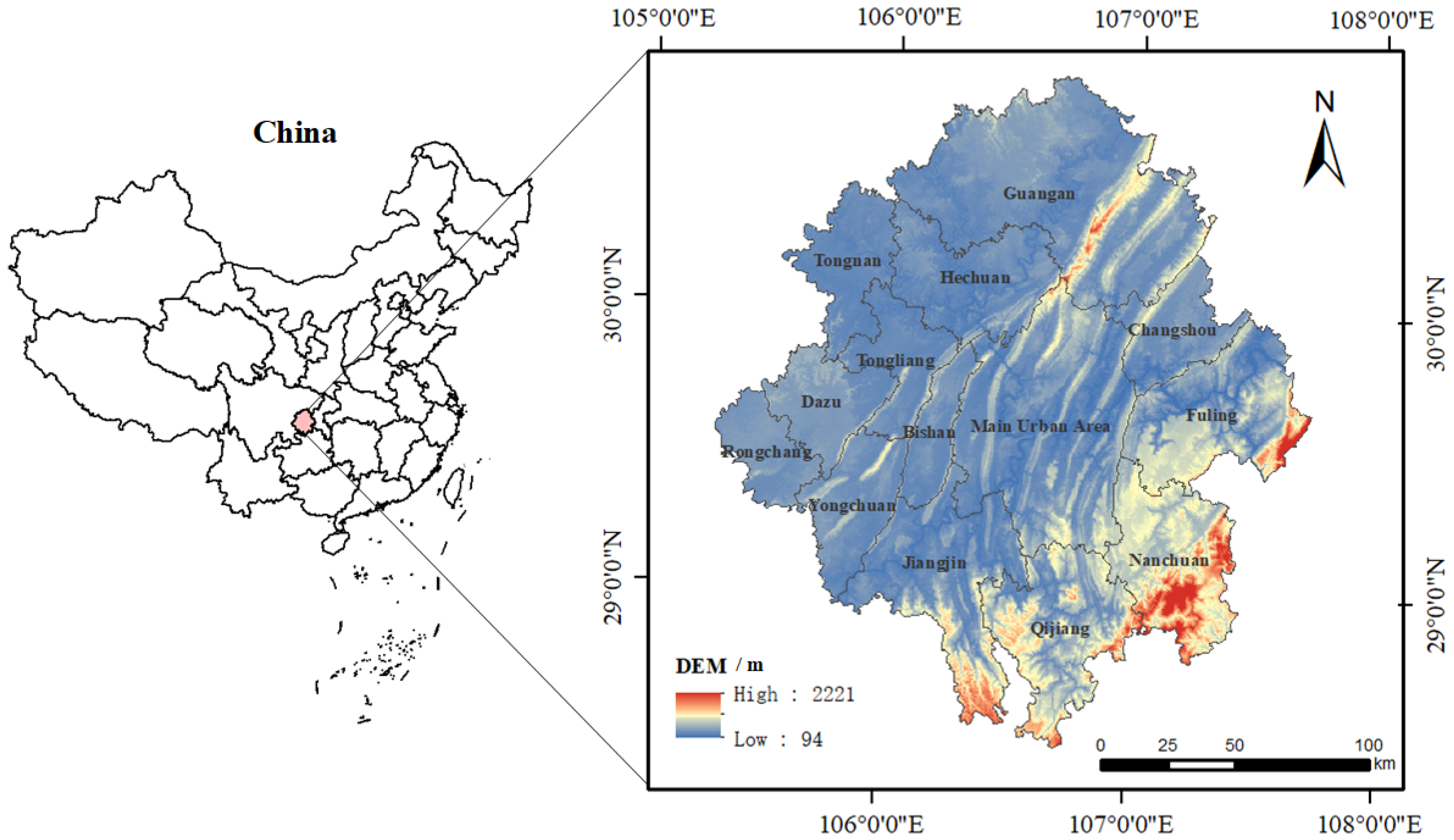
The Chongqing metropolitan area is located in the western part of Chongqing and the eastern part of the Chengdu–Chongqing urban agglomeration. It includes 21 districts, including the central urban area and the main urban new area of Chongqing as well as the entire administrative area of Guang’an City in Sichuan Province. The total area covers 35,000 square kilometers, and in 2020, the permanent population was 24.4 million people. The Chongqing metropolitan area is a significant urban cluster in the central-western region of China. In 2022, a development plan was approved by the National Development and Reform Commission and jointly issued by the People’s Government of Chongqing Municipality and the People’s Government of Sichuan Province under the title “Development Plan for the Chongqing Metropolitan Area”. This marks the first inter-provincial urban cluster planning initiative in the central-western region, signifying a crucial step in urbanization and economic cooperation in the area. The development of the Chongqing metropolitan area will serve as a vital engine for the overall development of the central-western region, demonstrating positive exemplary effects on regional cooperation and urban development at the national and international levels. The geographical location and scope of the study area are illustrated in Figure 1.
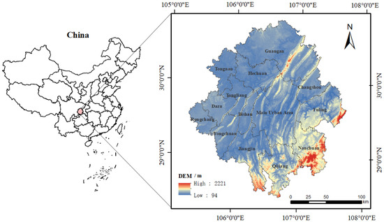
Figure 1.
The geographical location of the Chongqing metropolitan area.
2.2. Data Sources and Preprocessing
2.2.1. Data Types and Sources
In this study, land use data were obtained from the LUCC dataset provided by the Global Geospatial Information Products Platform. Based on the land use characteristics of the study area, land use types were classified into six categories: cultivated land, forest land, grassland, water bodies, construction land, and unused land. Land use change is a complex, dynamic process influenced by various factors. The original data sources are presented in Table 1. The Chongqing metropolitan area has a complex natural environment. In this study, the digital elevation model (DEM) and slope were used to characterize the natural environmental factors of the study area. DEM data were obtained from the ASTER GDEM V3 (30 m) dataset jointly developed by the National Aeronautics and Space Administration (NASA) and the Japan Aerospace Exploration Agency (JAXA), with the slope calculated from the DEM. Transportation network data were sourced from OpenStreetMap (OSM). Socio-economic conditions were primarily characterized by factors such as nighttime lights, population density, and point-of-interest (POI) density. Nighttime light data typically come from two channels: NPP/VIIRS and DMSP/OLS. However, due to different data years and compatibility issues between the two channels, the nighttime lights dataset created by Wu et al. [40] was used. This dataset was generated by integrating DMSP-OLS and SNPP-VIIRS data and correcting for discrepancies. Population density data were obtained from the WorldPop population density dataset. Point-of-interest data, including hospitals, schools, and living facilities, originated from the Gaode POI dataset.

Table 1.
Description of research data sources.
2.2.2. Data Processing
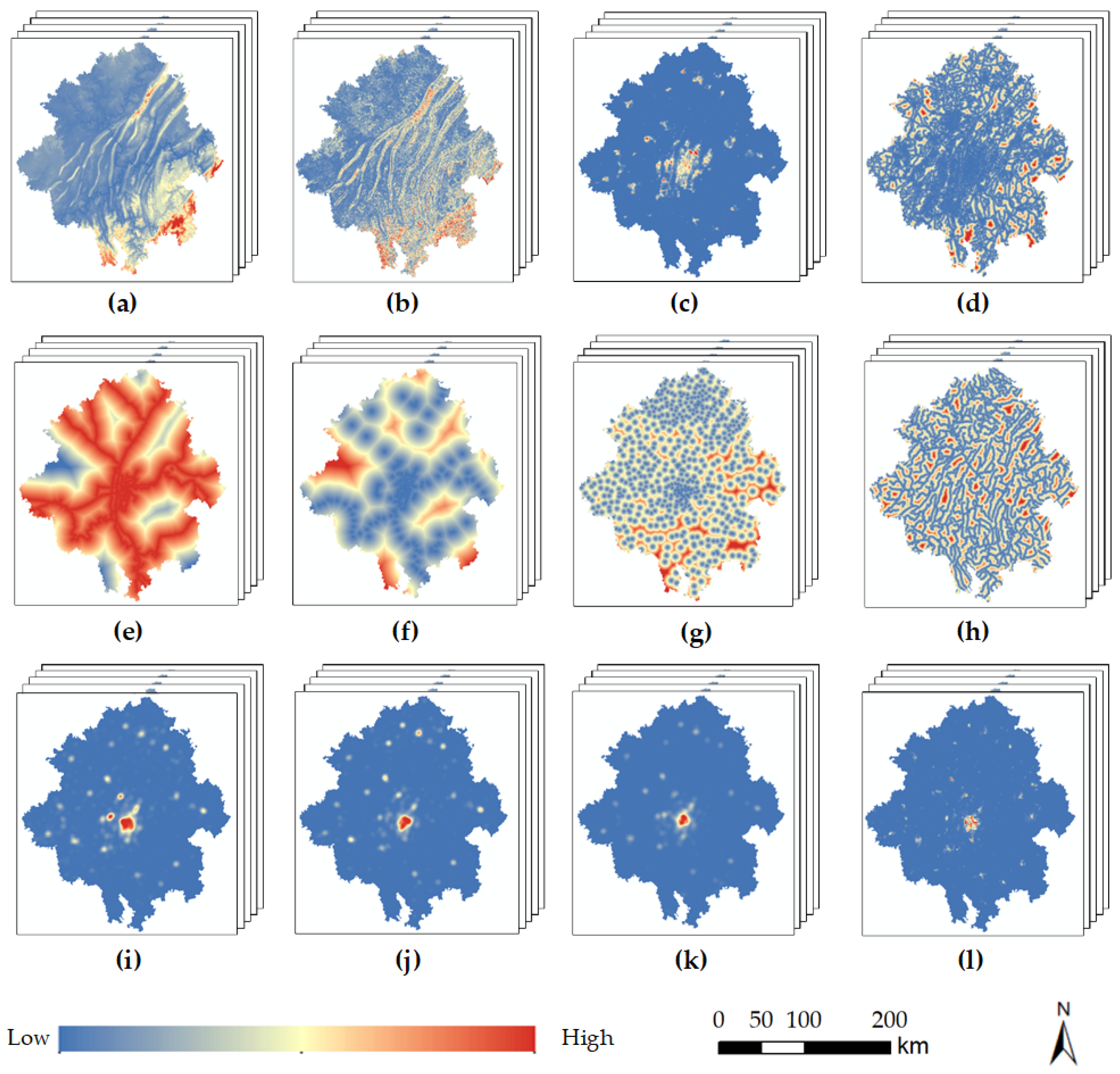
This study aims to explore the complex dependency relationships between the driving factor sequences and land use. Therefore, the selected driving factors should exhibit differentiation in global changes over time. Drawing on previous research in land use simulation, we comprehensively consider the influences of various factors, including natural environmental factors, transportation accessibility, and socio-economic conditions. A total of 12 driving factors were chosen, encompassing elevation, slope, nighttime lights, distance to major roads, distance to railways, distance to train stations, distance to town centers, distance to rivers, school point density, hospital point density, living facility point density, and population density. The processed sequence data are illustrated in Figure 2.
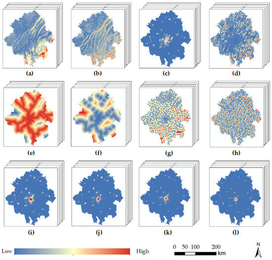
Figure 2.
Driving factors of LUCC: (a) DEM; (b) slope; (c) nighttime light; (d) distance to main road; (e) distance to railway; (f) distance to train station; (g) distance to town center; (h) distance to river; (i) density of schools; (j) density of hospitals; (k) density of amenities; (l) population.
Distance data were obtained through Euclidean distance analysis of road network data, while density data were derived through kernel density analysis of point-of-interest (POI) data. The original data for multiple periods of driving factors were collected over a two-year interval. After processing the data as described above, the unified and cropped datasets resulted in five periods of driving factor sequence data within the study area. To address potential spatial mismatch issues among different datasets, all data were uniformly resampled to a 100 m resolution, and the driving factors were normalized to [0, 1]. All data processing in this study was carried out using ArcMap 10.5 and Python 3.8 to ensure consistency and accuracy.
3. Methods
The overall framework of the VST-PCA model is illustrated in Figure 3, mainly comprising four components: the data processing module, the model training and prediction module, the dynamic iterative simulation module, and the model validation module. Firstly, the data processing module is responsible for handling the collected multi-source heterogeneous data, including data format conversion and resolution standardization. In this process, invalid values in the grid are removed, and a random stratified sampling of 5% of the data is performed to obtain 175,000 samples. The corresponding driving factor sequence data are obtained from these samples, forming the sample dataset. Among these samples, 70% are used as the training set for the next module, while the remaining 30% are reserved for model validation. The processed driving factor sequences and land use data are loaded into the model training and prediction module, which utilizes VST for feature extraction and connects to MLP to obtain the development suitability for each land use type for every grid. Subsequently, the dynamic iterative simulation module conducts simulations for LUCC, incorporating a pre-allocation strategy within the CA model. After each simulation round, if the land use requirements are not met, the rules of the pre-allocation strategy are adjusted, initiating the next simulation round. This process continues until the demands for all land categories are satisfied. Once this condition is met, the iteration is terminated, and the simulation results are output. Finally, the model validation module is responsible for evaluating the accuracy of the model.
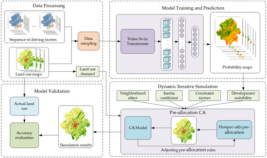
Figure 3.
Comprehensive framework of the VST-PCA model workflow.
3.1. Extract Transformation Rules Based on Spatiotemporal Feature Learning
Based on the learning of spatiotemporal features to explore the dependencies between LUCC and driving factors, we can more accurately extract transformation rules. This paper introduces an innovative deep learning model, namely, the video swin transformer (VST), based on spatiotemporal attention mechanisms to more effectively capture spatiotemporal dependencies. Unlike traditional 3DCNN video classification models that use 3D convolutional kernels to extract features, VST adopts a pure transformer architecture. Leveraging the self-attention mechanism in the transformer, this model comprehensively captures spatiotemporal dependencies throughout the entire video. Treating the video as a spatiotemporal sequence of image patches extracted from individual frames, VST utilizes the self-attention mechanism of the transformer to process these image patches, achieving a more comprehensive capture of spatiotemporal relationships in the video.
The swin transformer mimics the hierarchical mapping approach used by CNNs. In the initialization stage, the input image is segmented into non-overlapping blocks through the patch partition module, and adjacent blocks gradually merge into deeper transformer layers. By performing local self-attention computations within these non-overlapping windows, the swin transformer reduces the computational complexity from quadratic to linear. However, this partitioning leads to a reduction in connections for each window. To address this issue, the swin transformer introduces the concept of a sliding window to enhance information interaction between windows [41]. In this way, the model can better capture global features of the input image while maintaining lower computational complexity.
VST is essentially a three-dimensional extension of the swin transformer, strictly following the hierarchical structure of the swin transformer but expanding the scope of local attention computations from spatial to spatiotemporal domains. LUCC, to some extent, reflects the spatiotemporal dynamic variations of land use patterns and can be considered a special type of motion. Therefore, predicting future LUCC is akin to addressing a classification problem from a geographical perspective. In this context, the study regards a single-period driving factor as a frame image, while multiple-period driving factors are likened to a sequence of frames decomposed from a video. Consequently, VST can be utilized to extract the developmental suitability of each grid by treating these frames as spatiotemporal sequences. This extension into the spatiotemporal domain enables the model to more effectively capture the spatiotemporal features of changes in driving factors, resulting in a more accurate prediction of the future evolution of land use patterns.
This study employs a miniature version of VST (Swin-T) for feature extraction, and the overall architecture of the model is illustrated in Figure 4, divided into four stages for feature extraction. The size of the input sample’s driving factor data is defined as , where represents a sequence composed of periods. Each period contains grids, with and denoting the height and width of the input grid image, and representing the number of driving factors. After passing through the 3D patch partition layer, the input driving factor data is segmented into several 3D tokens. In Stage 1, a linear embedding layer projects the features of each token into an arbitrary dimension represented by C [42], which is then input into the VST block. In Stages 2, 3, and 4, the patch merging layer combines adjacent 2 × 2 patches, applying linear layers to achieve down sampling and feature doubling effects, followed by input into the VST block. Through the staged feature extraction process, the model gradually extracts and merges spatiotemporal feature information from the driving factor sequence.
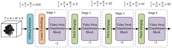
Figure 4.
Overall architecture of the video swin transformer.
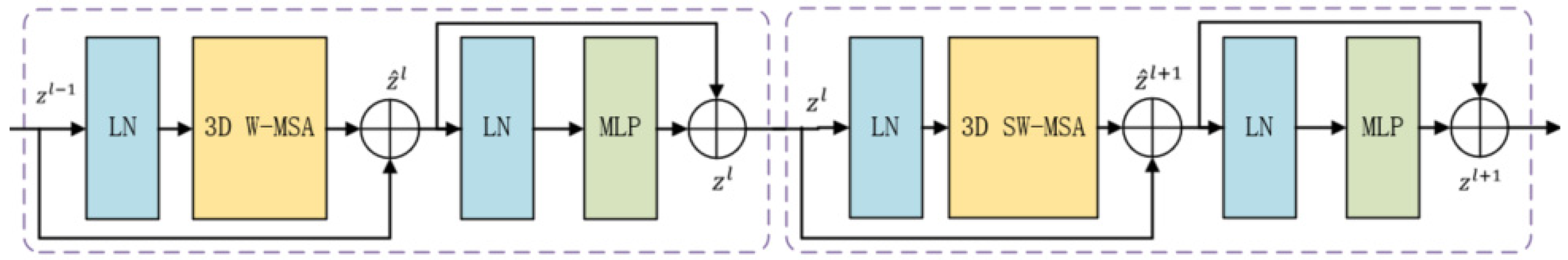
The main components of the model consist of the VST module, which is composed of an alternating 3D window multi-head self-attention (3D W-MSA) module and a 3D shifted-window multi-head self-attention (3D SW-MSA) module. The specific structure of the VST block and the connection between two consecutive VST blocks are illustrated in Figure 5. Each VST block is comprised of a 3D (shifted) window-based MSA module and an MLP. Layer normalization (LN) is applied before each MSA module and MLP module, and residual connections [43] are applied after each module. Based on the shifted-window partitioning method, the feature maps in two consecutive VST blocks are calculated as follows:
where and represent the output features of the 3D (S)W-MSA module and the MLP module of the -th block, respectively.
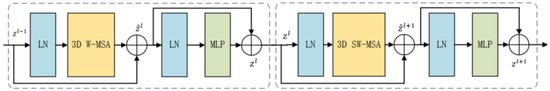
Figure 5.
The connection illustration of two consecutive video swin transformer blocks.
The final output features of the VST model will undergo processing through an MLP to generate probability distributions for six different land use types. All grid data are input into the model and processed to obtain the suitability layer for the development of each land type.
3.2. Dynamic Iterative Simulation of Coupling Pre-Allocation Strategy
3.2.1. The Overall Simulation Process
In the dynamic iterative simulation module, this study proposes a pre-allocation strategy and couples it with the CA model to simulate LUCC. The specific process of dynamic iterative simulation is illustrated in Figure 6.
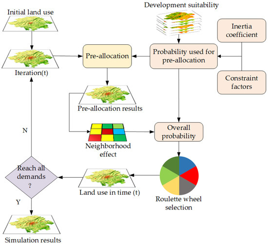
Figure 6.
The dynamic iterative process of the CA model coupled with a pre-allocation strategy.
In each iteration, we first calculate the probability on which pre-allocation depends. Subsequently, considering the demand for each land use, based on the principle of prioritizing the higher probability , we pre-allocate a certain proportion of land transformation for each land use type. The calculation method for is as follows:
where represents land development suitability generated by the VST model. represents the constraint factor, which restricts land changes in specified areas (such as open water bodies and some natural reserves) according to local policies. When a cell is within a restricted development area, the value of is 0; otherwise, it is 1. represents the inertia coefficient, whose main function is to dynamically increase the heritability of a specific land use type when the development trend of that type contradicts macro demand, ensuring consistency between the development trend of land use changes and future demand [44]. The calculation method for is as follows:
where is the inertia coefficient for type at the t-th iteration, is the coefficient at the (t − 1)th iteration, represents the difference between the allocation demand and the target demand for type at the (t − 1)th iteration, and represents the difference at the (t − 2)th iteration. When the evolutionary trend matches the macro demand, the inertia coefficient remains unchanged; otherwise, the inertia coefficient will be dynamically adjusted to correct the development trend in subsequent iterations [45].
After pre-allocation, the neighborhood effects are calculated based on the land use layers obtained from pre-allocation. Subsequently, the overall probability is determined by combining . The calculation methods for neighborhood effects and overall probability are defined as follows:
where represents the neighborhood effect for type at the t-th iteration. is the conditional function, taking the value 1 when the cell state is of type after pre-allocation and 0 otherwise. represents the overall probability for type at the t-th iteration, essentially calculated from , , , and .
The overall probability is applied to a roulette wheel selection mechanism to determine the target allocation type for cells. The principle of the roulette wheel selection mechanism in land use simulation involves constructing a roulette wheel based on the overall transition probabilities of various land use types. On this wheel, each sector represents a different land use type, with its area proportional to the transition probability of that land use type. The stopping position of the wheel is determined by generating a random number uniformly distributed between 0 and 1, thereby selecting a specific land use type. This random selection process ensures that land use types with higher probabilities have a greater chance of being selected, while those with lower probabilities still retain the possibility of selection. The random nature of this mechanism allows the model to reflect the uncertainty of real-world land use change dynamics [44,46]. In the end, the results of this iteration are obtained, and when the simulation results meet the overall demand, the model’s iteration will terminate; otherwise, it enters a new iteration.
3.2.2. Implementation Method of the Pre-Allocation Strategy
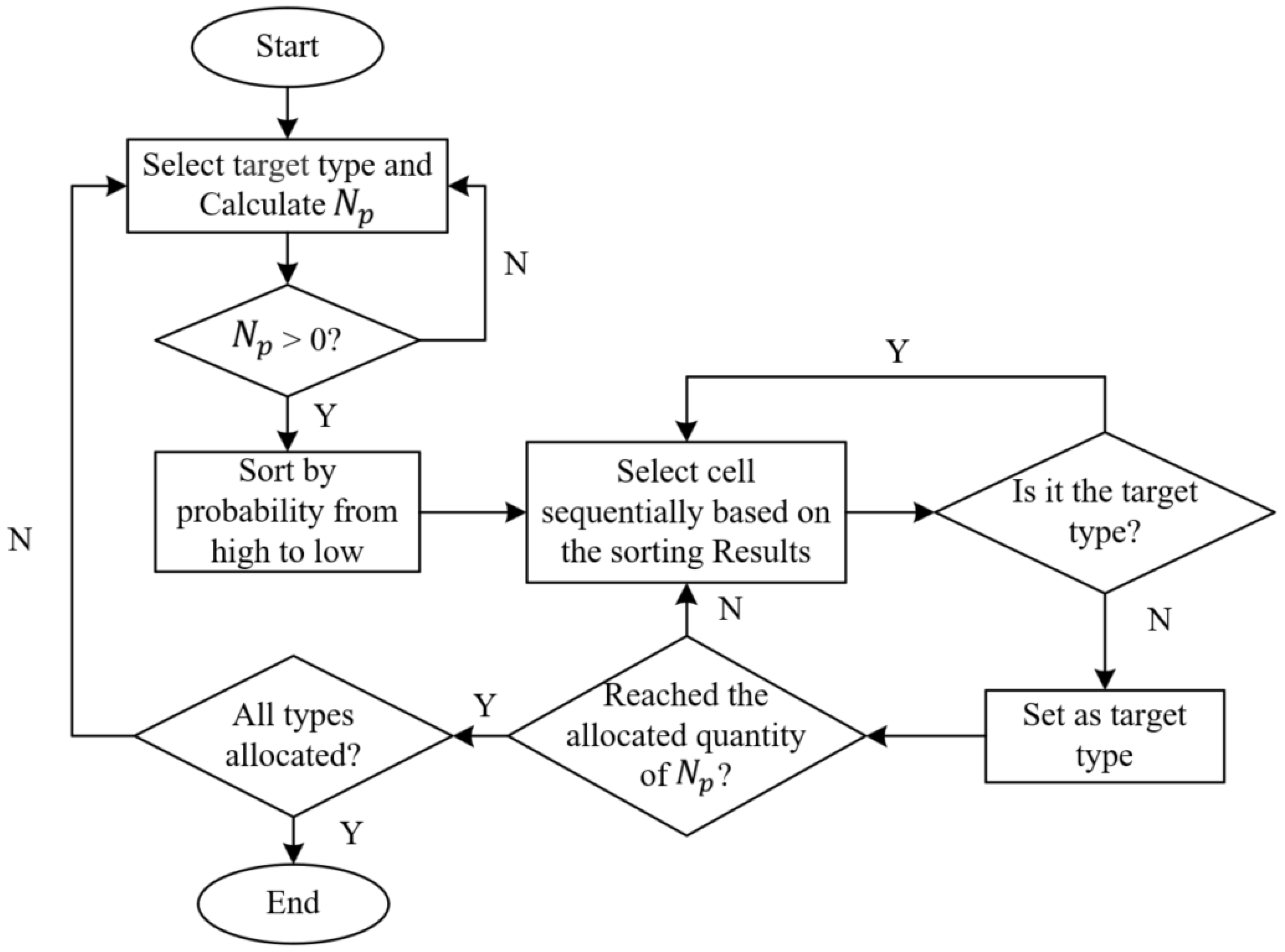
During land use simulation, CA models, by considering neighborhood effects, can exhibit spatially localized features. However, this local constraint may lead to a problem where, if a certain land use type does not exist in a particular area, even if the transition probability for that type is high, it may be challenging to simulate the occurrence of that land use type in subsequent simulations. The key issue with this phenomenon lies in overcoming the process from nonexistence to existence to ensure the smooth progression of subsequent simulations. In general, manually adding some cells at the beginning of the simulation or designing initialization rules can be considered. This paper proposes a strategy where, based on the priority principle of selecting cells with higher transition probability values , a portion of cells with higher transition probabilities is pre-allocated before each round of iterative simulation. These selected cells are referred to as “hotspot cells”. In this way, we can ensure the early appearance of land use types with higher transition probabilities in the simulation, thus avoiding difficulties in transitions during subsequent simulations. This approach facilitates the model to better reflect the real situation of LUCC.
The overall process of the pre-allocation strategy is illustrated in Figure 7. Specifically, the target type is sequentially chosen for allocation, excluding land use types with reduced demand from pre-allocation. Subsequently, the number of hotspot cells pre-allocated for target type are calculated; the cells are sorted in descending order based on the probability ; and then, according to the sorting results, cells of non-target types are consecutively selected for allocation until the allocated quantity reaches . After completing the pre-allocation for the current target type, we move on to the next target type, repeating the aforementioned steps until the pre-allocation for all types is completed. This yields the pre-allocation results for the current round of iterative simulation. The quantity for pre-allocating target type is defined as follows:
where represents the demand for land use type , represents the current quantity of land use type , and denotes the pre-allocation ratio. is a customizable parameter with a range of 0 to 1. A higher value indicates a greater influence of pre-allocation on the overall simulation. In this study, it was set to 0.1.

Figure 7.
Implementation flowchart of the pre-allocation strategy.
After the pre-allocation is completed, the current round of the CA model undergoes iterative simulation. The simulation continues until the demand for a certain land class is reached and the demand for all land uses is satisfied. If this condition is not met, the simulation proceeds to the next iteration, and the allocation ratio for the next round is adjusted. This process is repeated until the demand for all land uses is met. A mechanism similar to adjusting learning rates in deep learning is adopted to modify the pre-allocation ratio . gradually decreases with the number of iterations, allowing the impact of each round of pre-allocation to diminish in the overall iterative simulation, enabling a more natural evolution of the simulation. In this study, the pre-allocation ratio was adjusted through exponential decay, with a decay rate of 0.9.
3.3. Model Accuracy Evaluation
Based on relevant literature, this study selected overall accuracy (OA), Kappa coefficient, figure of merit (FOM), and F1 score to evaluate the accuracy of the constructed model. OA intuitively informs us about the accuracy of the model’s simulation across the entire study area, but when there is a class imbalance, overall accuracy may exhibit bias. The consideration of randomness in the Kappa coefficient makes it more robust, allowing for a better assessment of model performance in situations with different sample distributions and class imbalances. Therefore, it is widely used for evaluating land use classification or modeling [47]. The formula for calculating the Kappa coefficient is as follows:
where represents the number of correctly simulated grids, represents the total number of grids, represents the type of land use, represents the number of grids of land use type in actual observation data, and represents the number of grids of type in the prediction results.
The FOM index can comprehensively measure the modeling accuracy of simulated changes, as it focuses on the accuracy of the changing areas rather than the entire study area [48]. The range of FOM is from 0 to 1, where a higher FOM indicates a higher simulation accuracy. The calculation formula for the FOM index is as follows:
Here, A represents the number of grid cells where actual changes occurred but were not predicted to change, B represents the number of grid cells where actual changes occurred and were correctly predicted, C represents the number of grid cells where actual changes occurred and were captured as changes but were incorrectly predicted, and D represents the number of grid cells where actual changes did not occur but were predicted to change.
In this study, the F1 score was used to evaluate the simulation accuracy of each land use type. The F1 score is a harmonic mean that comprehensively considers precision and recall and is calculated as follows:
where represents the number of true positive predictions (correctly predicted positive samples), represents the number of false positive predictions (negative samples incorrectly predicted as positive), and represents the number of false negative predictions (positive samples incorrectly predicted as negative).
4. Results
4.1. Evaluation of Development Suitability Maps
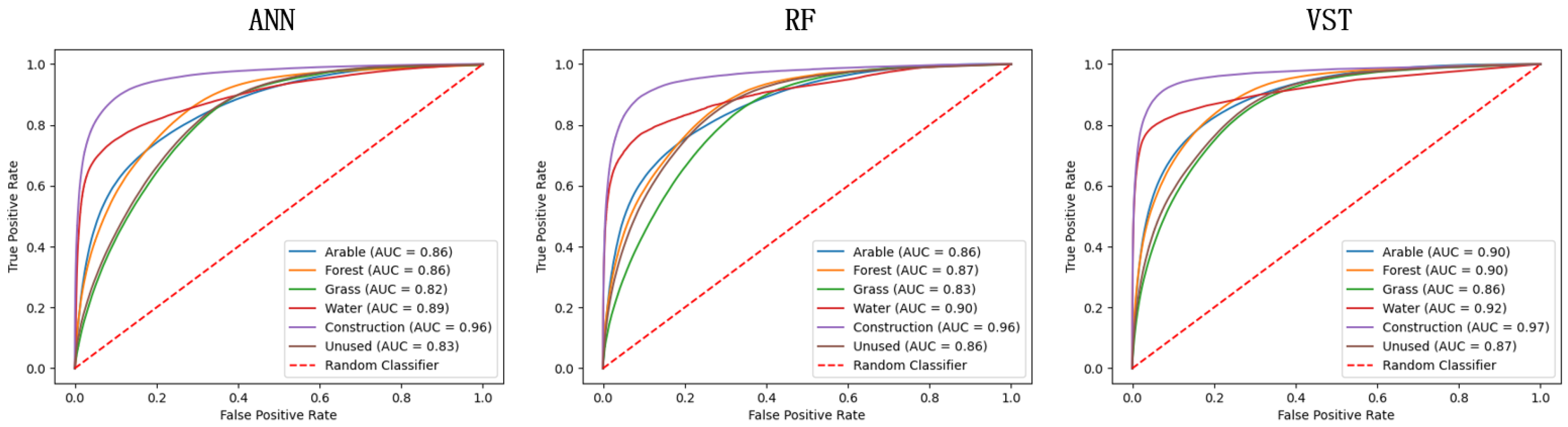
A development suitability map is a spatial visualization layer generated based on conversion rules. Development suitability reveals the spatial distribution and patterns of land use changes. Accurate land development suitability ensures that the simulation reflects the trends and patterns of actual land use changes, directly impacting the simulation accuracy of the model. If the extracted development suitability is not accurate, it may significantly reduce the accuracy of the simulation. Receiver operating characteristic (ROC) curves and area under the curve (AUC) values have been proven useful for evaluating the quality of development suitability maps in CA models [48]. The ROC curve is created by plotting the true positive rate (TPR, sensitivity in machine learning) against the false positive rate (FPR, estimated by 1 - specificity) at various threshold selections [44]. In theory, if the AUC value is closer to 1, indicating a larger area under the curve, it signifies a higher accuracy of the predictive model. Conversely, a lower AUC value suggests lower accuracy. When AUC is 1.0, it indicates a perfect classifier model.
After processing the data through the data processing module, a unified dataset is obtained. In this study, 5% of the data was randomly stratified as samples, resulting in a final set of 175,000 samples. Among these, 70% of the samples were used as the training set, while the remaining 30% were used for model validation. Table 2 presents detailed information about the dataset. Currently, most research related to LUCC simulation tends to use traditional machine learning models as tools for extracting development suitability, and these models are favored by researchers for their simplicity and efficiency. In this regard, we compared the development suitability maps generated in this study with those generated by ANN and RF. The ROC curves for each model are shown in Figure 8, where the red dashed line represents a random classifier. Table 3 lists the AUC values for the development suitability maps generated by each model. The results indicate that the VST model used in this study achieved the best performance across various land use types. The AUC values for cropland, forest land, water bodies, and construction land all exceeded 0.9, demonstrating that VST can generate more accurate development suitability maps, laying the foundation for subsequent simulation stages and improving the predictive performance of the model.
Table 2.
The elements of the dataset.
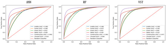
Figure 8.
ROC curves of each model.
Table 3.
AUC values of each model.
4.2. Model Accuracy Comparison
4.2.1. Comparison of Accuracy with Mainstream Models
To validate the effectiveness of the model, this study constructed two traditional CA models, namely, ANN-CA and RF-CA, as well as two deep learning CA models that consider spatiotemporal dependencies, namely, CNN-LSTM-CA [19,31] and ST-CA [23]. These models were compared in detail with the VST-PCA model proposed in this paper. Table 4 presents the accuracy comparison of each model.
Table 4.
Comparison of simulation accuracy among different models.
According to the data in Table 4, we can observe that the accuracy of the two traditional CA models (ANN-CA and RF-CA) was relatively low. The widespread application of traditional machine learning models is mainly attributed to their simplicity and ease of use, and therefore, their lower complexity may limit their performance in handling complex data patterns, resulting in lower simulated accuracy. In contrast, the two deep learning models (CNN-LSTM-CA and ST-CA) showed a significant improvement in performance. This indirectly proves the effectiveness of deep learning models in extracting spatiotemporal dependencies. These models take into account the complex spatiotemporal dependencies between land use and driving factors, allowing them to better capture complex features and patterns in the data, resulting in superior simulation performance. The VST-PCA model proposed in this paper achieved the best results among the compared models, with an overall accuracy (OA) of 0.9311, a Kappa coefficient of 0.8654, and a figure of merit (FOM) index reaching 0.4534. Compared to other models, the Kappa coefficient increased by 0.0322–0.1036, and the FOM index increased by 0.0513–0.1649. The outstanding performance of the model validates the effectiveness of the model proposed in this paper.
Table 5 presents the F1 score for each land use type. Similar to the overall accuracy, VST-PCA performed the best in terms of simulation effectiveness, further validating the effectiveness of the model proposed in this paper. In terms of land use types, cropland and construction land exhibited higher simulation accuracy. However, in the case of grassland, although VST-PCA showed some improvement in accuracy compared to other models, it still remained relatively low compared to other land use types. This phenomenon is attributed to specific geographical and land use characteristics in the region. A detailed analysis revealed that grassland was mainly distributed in the southeastern region of the Chongqing metropolitan area, where various land use types exhibited a more fragmented and scattered distribution pattern. This dispersion posed a greater challenge for the model when predicting and simulating grassland because of the higher likelihood of overlap between grassland and other land use types, making it difficult to clearly delineate boundaries and ultimately resulting in a decrease in simulation accuracy.
Table 5.
F1 scores for each land use type in each model.
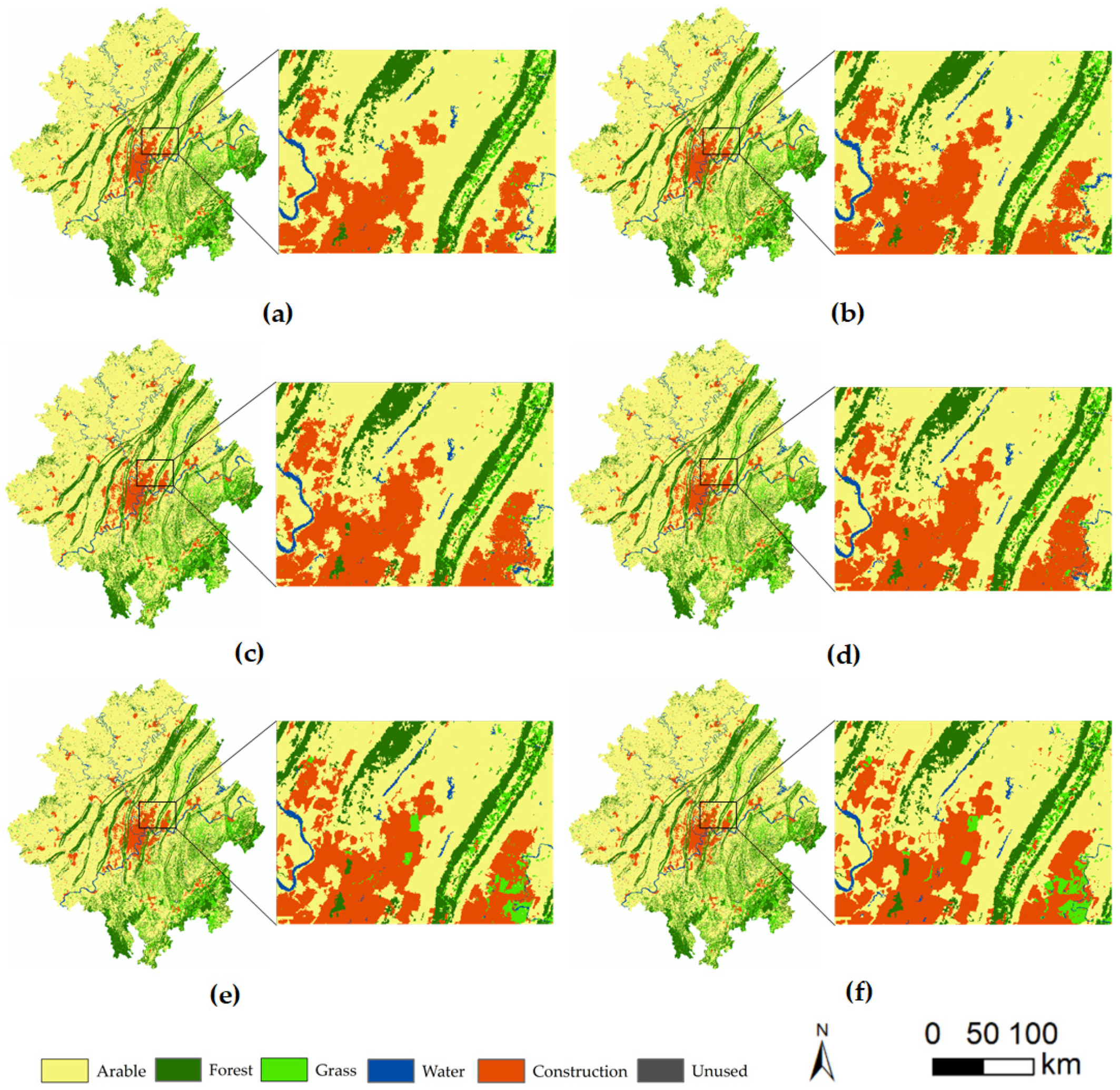
Figure 9 illustrates the simulation results of each model, focusing on a relatively typical region to demonstrate the differences in the simulated outcomes of each model. From the figure, it can be observed that the simulation results generated by the proposed VST-PCA model better reflected the current land use status and demonstrated superior performance in terms of detail. During the period from 2010 to 2020, significant changes in land use occurred in the selected region, particularly with the emergence of multiple grassland areas showing a development trend of “from absence to presence”. This complex change made the performance of other models relatively poorer, while the VST-PCA model, with its adopted cellular pre-allocation strategy, achieved more realistic and accurate simulation results. The VST-PCA model excelled at capturing land use changes, and its cellular pre-allocation strategy contributed to better simulating the formation of emerging areas. This example region highlights the unique advantage of the VST-PCA model in handling dynamic land use changes.
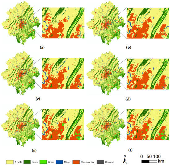
Figure 9.
Comparison of land use simulation results and actual results in 2020: (a) simulation results of ANN-CA; (b) simulation results of RF-CA; (c) simulation results of CNN-LSTM-CA; (d) simulation results of ST-CA; (e) simulation results of VST-PCA; (f) actual LU map.
4.2.2. Ablation Studies
To validate the effectiveness of the VST-PCA modules, we constructed multiple models for ablation studies, including (1) RF-CA, serving as a baseline model, using random forest (RF) to generate development suitability maps without incorporating pre-allocation strategies; (2) VST-CA, utilizing VST to generate development suitability maps without employing pre-allocation strategies; (3) RF-PCA, employing RF to generate development suitability maps and incorporating pre-allocation strategies; and (4) VST-PCA, the complete model incorporating all key modules.
The ablation experiment results are shown in Table 6. In both VST-CA and VST-PCA, we employed VST to extract spatiotemporal dependencies and generate suitability maps for development, replacing the traditional RF model in the baseline. Without using a pre-allocation strategy for simulation, VST-CA increased the Kappa coefficient and FOM index of the simulated results from 0.7702 and 0.2905 to 0.8501 and 0.4167, respectively, representing improvements of 0.0799 and 0.1262. When using a pre-allocation strategy for simulation, VST-PCA increased the Kappa coefficient and FOM index of the simulated results from 0.8137 and 0.3622 to 0.8654 and 0.4534, respectively, showing improvements of 0.0517 and 0.0912.
Table 6.
Comparison of ablation models.
In RF-PCA, RF is employed to generate development suitability maps, but a pre-allocation strategy is incorporated to address issues arising from neighborhood effects in CA simulations. The introduction of the pre-allocation strategy resulted in an improvement in the Kappa coefficient and FOM index of the simulation results, increasing from 0.7702 and 0.2905 to 0.8137 and 0.3622, respectively, representing improvements of 0.0435 and 0.0717. When using the VST model, compared to simulations without the pre-allocation strategy, the results with the pre-allocation strategy showed that the Kappa coefficient and FOM index increased from 0.8501 and 0.4167 to 0.8654 and 0.4534, respectively, representing improvements of 0.0153 and 0.0367.
From the perspective of the Kappa coefficient, overall, the improvement in spatiotemporal effects resulted in a performance enhancement ranging from 5.17% to 7.99%, while the improvement in pre-allocation effects manifested as an increase of 1.53% to 4.35%. Simultaneously, from the perspective of the FOM index, the enhancement in spatiotemporal effects led to a performance improvement ranging from 9.12% to 12.62%, and the improvement in pre-allocation effects also resulted in a performance increase of 3.67% to 7.17%. The results indicate that the improvements made to both components of VST-PCA are beneficial for the construction of land use simulation models.
4.3. Time Performance Evaluation and Analysis
A comparative analysis of the temporal performance of different models was conducted to further evaluate our proposed VST-PCA model. LUCC prediction simulations generally consist of two stages, namely, the suitability extraction stage and the simulation stage. We evaluated these two stages separately. All comparative experiments were based on the same hardware foundation.
Table 7 presents the time consumption for each model during the development suitability extraction stage. Model-specific parameter settings were as follows: ANN had two hidden layers with 256 neurons in each layer; RF comprised 800 decision trees with a maximum depth of 40; and the parameters for CNN-LSTM and 3DCNN were adopted from existing literature. In terms of time consumption, both ANN-CA and RF-CA exhibited lower time requirements, while deep learning-based CA models necessitated longer processing times—sometimes even dozens of times higher than RF-CA. While acknowledging that using time consumption as the sole evaluation indicator may have some limitations, the experimental results generally reflect the overall trend in model performance. Despite the notable accuracy improvements achieved by the three deep learning-based CA models, this comes at the expense of higher computational costs. Among these models, the ST-CA model is the most time-consuming. This is primarily because the ST-CA model employs 3DCNN to extract spatiotemporal dependencies. By extending convolutional layers along the temporal dimension, 3DCNN can directly handle and learn the spatiotemporal features of sequential data. While this model effectively captures temporal dynamics when processing sequential data, it typically involves a large number of parameters and computations, resulting in higher time consumption.
Table 7.
Model development suitability extraction time comparison.
Table 8 shows the time consumption during the simulation stage, where Model I incorporated the pre-allocation strategy during iterative simulations, while Model II did not utilize the pre-allocation strategy. Both approaches were based on the same development suitability map and overall simulation requirements. Multiple experiments were conducted for different development suitability maps, and the average time consumption was taken as the result. The research results indicated that the time consumption of Model I was significantly lower than that of Model II, suggesting that the pre-allocation strategy can enhance simulation efficiency to a certain extent. Before each iteration of simulation, the pre-allocation strategy rapidly assigns a portion of the requirements, aiding in the quicker exploration of new areas and faster fulfillment of simulation needs. This effectively reduces the overall time of the simulation.
Table 8.
Comparison of simulation time consumption.
5. Discussion
The VST-PCA model utilizes the video swin transformer to deeply learn spatiotemporal features, which is a promising attempt at LUCC simulation. This approach surpasses traditional CA models in accurately capturing the complex dynamics of land use changes. While recent studies have integrated deep learning techniques, the VST-PCA model excels at capturing long-term and complex spatiotemporal dependencies, reflected in improved simulation accuracy. However, it is undeniable that deep learning-based CA models are generally time-consuming, and achieving high precision with low time consumption remains a challenging issue. Introducing a pre-allocation strategy is a major innovation of the VST-PCA model, optimizing the simulation process of land use changes in traditional CA models. Compared to previous research, the VST-PCA model significantly enhances simulation accuracy and practicality through this strategy, demonstrating its powerful capability in simulating complex geographical processes in real-world applications. By comparing the VST-PCA model with other CA-based models, its advantages in simulation precision and detail capture are evident. The VST-PCA model predicts land use dynamics more accurately than other models based on traditional machine learning and deep learning, especially in capturing long-term trends and subtle spatial changes.
Despite the significant effects achieved by VST-PCA, there are still aspects worthy of further discussion. Firstly, the model has relatively strict requirements for driving factor data, and obtaining the extensive and long-term time series data the model needs is challenging. In future work, it may be worth considering methods for predicting driving factor data to access a broader range of long-term time series data. Additionally, as a deep learning model, although VST shows some improvement in training speed, its cost remains relatively high compared to traditional machine learning models. In future work, it will be necessary to consider how to enhance simulation accuracy while minimizing associated computational costs. This requires further optimization of the model and more efficient utilization of computational resources.
6. Conclusions
This paper introduces a novel land use change simulation model, VST-PCA, which integrates two key modules: spatiotemporal feature learning and pre-allocation strategy. Through extensive ablation studies and comparative analysis with existing models, this research not only validates the accuracy and effectiveness of the VST-PCA model but also highlights its unique contributions and advantages in the LUCC simulation domain.
The VST-PCA model employs VST to extract complex spatiotemporal features, thereby capturing the temporal and spatial dependencies between driving factors and land use more accurately, resulting in more precise suitability maps for development. The land development suitability maps produced by this method are significantly superior to those generated by traditional approaches, with AUC values for all land use types exceeding 0.8. For cropland, forest land, water bodies, and built-up areas, the AUC values were no less than 0.9, providing a solid foundation for subsequent simulations.
The pre-allocation strategy introduced in VST-PCA optimizes the spatial simulation stage and addresses the constraints of conventional neighborhood effect calculations. Especially in the expansion of new districts, this strategy improves the model’s representation and accuracy by identifying and prioritizing areas with high transition probabilities. This approach demonstrated superior performance in specific regions compared to other models, underscoring the importance of the pre-allocation strategy.
Using LUCC observation data from the Chongqing metropolitan area from 2010 to 2020 as an example, this study conducted an in-depth performance evaluation of the VST-PCA model, confirming its superior performance compared to other models through comparative analysis. The results show that the VST-PCA model significantly outperformed other models, with Kappa coefficients and FOM indices reaching 0.8654 and 0.4534, respectively. The exceptional performance of the VST-PCA model is attributed not only to its fine-grained spatiotemporal feature extraction capability but also to its unique land pre-allocation strategy. Notably, the precision improvement offered by VST-PCA is not a simple additive effect of spatiotemporal and configuration effects. The precision gain from pre-allocation is clearly less than the improvement brought by the spatiotemporal effect of adopting the VST model. By employing land pre-allocation, the model not only enhances accuracy but also contributes to improved simulation operational efficiency. Moreover, it represents a method that more closely aligns with actual land conversion processes. The application of the VST-PCA model not only elevates the precision of LUCC simulations but also provides a new direction for future research, namely, exploring the potential of spatiotemporal feature learning in geospatial simulation. This approach offers a powerful and flexible tool for understanding and predicting land use changes, aiding more accurate decision-making in urban planning, ecological conservation, and climate change studies, among other fields.
Author Contributions
Conceptualization, Minghao Liu and Qingxi Luo; methodology, Qingxi Luo; software, Qingxi Luo; validation, Minghao Liu and Jianxiang Wang; formal analysis, Minghao Liu and Qingxi Luo; investigation, Qingxi Luo and Jianxiang Wang; resources, Lingbo Sun, Tingting Xu and Qingxi Luo; data curation, Qingxi Luo; writing—original draft preparation, Qingxi Luo; writing—review and editing, Minghao Liu and Lingbo Sun; visualization, Qingxi Luo and Enming Wang; supervision, Minghao Liu and Tingting Xu; project administration, Tingting Xu; funding acquisition, Tingting Xu. All authors have read and agreed to the published version of the manuscript.
Funding
This research was funded by the National Natural Science Foundation of China, grant number 42071218 and Chongqing Doctor Through Train Project “Research on 5G Base Station Planning and Deployment System Based on City Information Modeling (CIM)”, grant number CSTB2022BSXM-JCX0147.
Data Availability Statement
Data are contained within the article.
Acknowledgments
The authors would like to acknowledge the editors and reviewers of the ISPRS International Journal of Geo-Information for their constructive comments and suggestions, and extend a special thanks to Chun Chen for her significant contributions to the research.
Conflicts of Interest
The authors declare no conflicts of interest.
References
- Dadashpoor, H.; Azizi, P.; Moghadasi, M. Land Use Change, Urbanization, and Change in Landscape Pattern in a Metropolitan Area. Sci. Total Environ. 2019, 655, 707–719. [Google Scholar] [CrossRef] [PubMed]
- Wang, G.; Han, Q. The Multi-Objective Spatial Optimization of Urban Land Use Based on Low-Carbon City Planning. Ecol. Indic. 2021, 125, 107540. [Google Scholar] [CrossRef]
- Yi, Y.; Zhang, C.; Zhu, J.; Zhang, Y.; Sun, H.; Kang, H. Spatio-Temporal Evolution, Prediction and Optimization of LUCC Based on CA-Markov and InVEST Models: A Case Study of Mentougou District, Beijing. Int. J. Environ. Res. Public Health 2022, 19, 2432. [Google Scholar] [CrossRef] [PubMed]
- Xiao, Y.; Guo, B.; Lu, Y.; Zhang, R.; Zhang, D.; Zhen, X.; Chen, S.; Wu, H.; Wei, C.; Yang, L.; et al. Spatial–Temporal Evolution Patterns of Soil Erosion in the Yellow River Basin from 1990 to 2015: Impacts of Natural Factors and Land Use Change. Geomat. Nat. Hazards Risk 2021, 12, 103–122. [Google Scholar] [CrossRef]
- Li, S.; Liu, X.; Li, X.; Chen, Y. Simulation Model of Land Use Dynamics and Application: Progress and Prospects. J. Remote Sens 2017, 21, 329–340. [Google Scholar] [CrossRef]
- Li, X.; Yeh, A.G.-O. Neural-Network-Based Cellular Automata for Simulating Multiple Land Use Changes Using GIS. Int. J. Geogr. Inf. Sci. 2002, 16, 323–343. [Google Scholar] [CrossRef]
- Okwuashi, O.; Ndehedehe, C.E. Integrating Machine Learning with Markov Chain and Cellular Automata Models for Modelling Urban Land Use Change. Remote Sens. Appl. Soc. Environ. 2021, 21, 100461. [Google Scholar] [CrossRef]
- Yuhong, G.; Lijuan, Z.; Wenliang, L. Urban Expansion Simulation Using GIS Spatial Analysis and Cellular Automata. Sci. Geogr. Sin. 2010, 30, 723–727. [Google Scholar]
- Kamusoko, C.; Gamba, J. Simulating Urban Growth Using a Random Forest-Cellular Automata (RF-CA) Model. ISPRS Int. J. Geo-Inf. 2015, 4, 447–470. [Google Scholar] [CrossRef]
- Lv, J.; Wang, Y.; Liang, X.; Yao, Y.; Ma, T.; Guan, Q. Simulating Urban Expansion by Incorporating an Integrated Gravitational Field Model into a Demand-Driven Random Forest-Cellular Automata Model. Cities 2021, 109, 103044. [Google Scholar] [CrossRef]
- Dang, X.; Zhou, L.; Li, X.; Mu, H.; Che, L.; Qiao, F. Simulation and Prediction of Shanghai Urban Spatial Change Based on Random Forest and CA-Markov Model. Abstr. ICA 2019, 1, 53. [Google Scholar] [CrossRef]
- Yang, Q.; Li, X.; Shi, X. Cellular Automata for Simulating Land Use Changes Based on Support Vector Machines. Comput. Geosci. 2008, 34, 592–602. [Google Scholar] [CrossRef]
- Zhang, X.; Zhou, J.; Song, W. Simulating Urban Sprawl in China Based on the Artificial Neural Network-Cellular Automata-Markov Model. Sustainability 2020, 12, 4341. [Google Scholar] [CrossRef]
- Omrani, H.; Tayyebi, A.; Pijanowski, B. Integrating the Multi-Label Land-Use Concept and Cellular Automata with the Artificial Neural Network-Based Land Transformation Model: An Integrated ML-CA-LTM Modeling Framework. GISci. Remote Sens. 2017, 54, 283–304. [Google Scholar] [CrossRef]
- Zhong, C.; Bei, Y.; Gu, H.; Zhang, P. Spatiotemporal Evolution of Ecosystem Services in the Wanhe Watershed Based on Cellular Automata (CA)-Markov and InVEST Models. Sustainability 2022, 14, 13302. [Google Scholar] [CrossRef]
- Collados-Lara, A.-J.; Pardo-Igúzquiza, E.; Pulido-Velazquez, D. Assessing the Impact of Climate Change–and Its Uncertainty–on Snow Cover Areas by Using Cellular Automata Models and Stochastic Weather Generators. Sci. Total Environ. 2021, 788, 147776. [Google Scholar] [CrossRef] [PubMed]
- Liu, Y.; He, Q.; Tan, R.; Liu, Y.; Yin, C. Modeling Different Urban Growth Patterns Based on the Evolution of Urban Form: A Case Study from Huangpi, Central China. Appl. Geogr. 2016, 66, 109–118. [Google Scholar] [CrossRef]
- Feng, Y.; Tong, X. Using Exploratory Regression to Identify Optimal Driving Factors for Cellular Automaton Modeling of Land Use Change. Environ. Monit. Assess. 2017, 189, 515. [Google Scholar] [CrossRef] [PubMed]
- Zhou, Y.; Huang, C.; Wu, T.; Zhang, M. A Novel Spatio-Temporal Cellular Automata Model Coupling Partitioning with CNN-LSTM to Urban Land Change Simulation. Ecol. Model. 2023, 482, 110394. [Google Scholar] [CrossRef]
- Wu, X.; Liu, X.; Zhang, D.; Zhang, J.; He, J.; Xu, X. Simulating Mixed Land-Use Change under Multi-Label Concept by Integrating a Convolutional Neural Network and Cellular Automata: A Case Study of Huizhou, China. GISci. Remote Sens. 2022, 59, 609–632. [Google Scholar] [CrossRef]
- White, R.; Engelen, G. Cellular Automata and Fractal Urban Form: A Cellular Modelling Approach to the Evolution of Urban Land-Use Patterns. Environ. Plan. A 1993, 25, 1175–1199. [Google Scholar] [CrossRef]
- Liu, X.; Li, X.; Yeh, A.G.-O.; He, J.; Tao, J. Discovery of Transition Rules for Geographical Cellular Automata by Using Ant Colony Optimization. Sci. China Ser. D Earth Sci. 2007, 50, 1578–1588. [Google Scholar] [CrossRef]
- Geng, J.; Shen, S.; Cheng, C.; Dai, K. A Hybrid Spatiotemporal Convolution-Based Cellular Automata Model (ST-CA) for Land-Use/Cover Change Simulation. Int. J. Appl. Earth Obs. Geoinf. 2022, 110, 102789. [Google Scholar] [CrossRef]
- Liu, M.; Chen, H.; Qi, L.; Chen, C. LUCC Simulation Based on RF-CNN-LSTM-CA Model with High-Quality Seed Selection Iterative Algorithm. Appl. Sci. 2023, 13, 3407. [Google Scholar] [CrossRef]
- Zhao, X.; Wang, P.; Gao, S.; Yasir, M.; Islam, Q.U. Combining LSTM and PLUS Models to Predict Future Urban Land Use and Land Cover Change: A Case in Dongying City, China. Remote Sens. 2023, 15, 2370. [Google Scholar] [CrossRef]
- He, J.; Li, X.; Yao, Y.; Hong, Y.; Jinbao, Z. Mining Transition Rules of Cellular Automata for Simulating Urban Expansion by Using the Deep Learning Techniques. Int. J. Geogr. Inf. Sci. 2018, 32, 2076–2097. [Google Scholar] [CrossRef]
- Zhai, Y.; Yao, Y.; Guan, Q.; Liang, X.; Li, X.; Pan, Y.; Yue, H.; Yuan, Z.; Zhou, J. Simulating Urban Land Use Change by Integrating a Convolutional Neural Network with Vector-Based Cellular Automata. Int. J. Geogr. Inf. Sci. 2020, 34, 1475–1499. [Google Scholar] [CrossRef]
- Gounaridis, D.; Chorianopoulos, I.; Symeonakis, E.; Koukoulas, S. A Random Forest-Cellular Automata Modelling Approach to Explore Future Land Use/Cover Change in Attica (Greece), under Different Socio-Economic Realities and Scales. Sci. Total Environ. 2019, 646, 320–335. [Google Scholar] [CrossRef] [PubMed]
- Liu, J.; Xiao, B.; Li, Y.; Wang, X.; Bie, Q.; Jiao, J. Simulation of Dynamic Urban Expansion under Ecological Constraints Using a Long Short Term Memory Network Model and Cellular Automata. Remote Sens. 2021, 13, 1499. [Google Scholar] [CrossRef]
- Wang, H.; Zhao, X.; Zhang, X.; Wu, D.; Du, X. Long Time Series Land Cover Classification in China from 1982 to 2015 Based on Bi-LSTM Deep Learning. Remote Sens. 2019, 11, 1639. [Google Scholar] [CrossRef]
- Xing, W.; Qian, Y.; Guan, X.; Yang, T.; Wu, H. A Novel Cellular Automata Model Integrated with Deep Learning for Dynamic Spatio-Temporal Land Use Change Simulation. Comput. Geosci. 2020, 137, 104430. [Google Scholar] [CrossRef]
- Xiao, B.; Liu, J.; Jiao, J.; Li, Y.; Liu, X.; Zhu, W. Modeling Dynamic Land Use Changes in the Eastern Portion of the Hexi Corridor, China by Cnn-Gru Hybrid Model. GISci. Remote Sens. 2022, 59, 501–519. [Google Scholar] [CrossRef]
- Tobler, W.R. Cellular Geography. Philos. Geogr. 1979, 379–386. [Google Scholar] [CrossRef]
- Zhai, S.; Feng, Y.; Yan, X.; Wei, Y.; Wang, R.; Li, P. Using Spatial Heterogeneity to Strengthen the Neighbourhood Effects of Urban Growth Simulation Models. J. Spat. Sci. 2023, 68, 319–337. [Google Scholar] [CrossRef]
- Moreno, N.; Wang, F.; Marceau, D.J. Implementation of a Dynamic Neighborhood in a Land-Use Vector-Based Cellular Automata Model. Comput. Environ. Urban Syst. 2009, 33, 44–54. [Google Scholar] [CrossRef]
- Zhang, B.; Wang, H. A New Type of Dual-Scale Neighborhood Based on Vectorization for Cellular Automata Models. GISci. Remote Sens. 2021, 58, 386–404. [Google Scholar] [CrossRef]
- Zhang, B.; Hu, S.; Wang, H.; Zeng, H. A Size-Adaptive Strategy to Characterize Spatially Heterogeneous Neighborhood Effects in Cellular Automata Simulation of Urban Growth. Landsc. Urban Plan. 2023, 229, 104604. [Google Scholar] [CrossRef]
- Pan, X.; Wang, Z.; Huang, M.; Liu, Z. Improving an Urban Cellular Automata Model Based on Auto-Calibrated and Trend-Adjusted Neighborhood. Land 2021, 10, 688. [Google Scholar] [CrossRef]
- Wang, J.; Hadjikakou, M.; Hewitt, R.J.; Bryan, B.A. Simulating Large-Scale Urban Land-Use Patterns and Dynamics Using the U-Net Deep Learning Architecture. Comput. Environ. Urban Syst. 2022, 97, 101855. [Google Scholar] [CrossRef]
- Wu, Y.; Shi, K.; Chen, Z.; Liu, S.; Chang, Z. Developing Improved Time-Series DMSP-OLS-Like Data (1992–2019) in China by Integrating DMSP-OLS and SNPP-VIIRS. IEEE Trans. Geosci. Remote Sens. 2022, 60, 1–14. [Google Scholar] [CrossRef]
- Liu, Z.; Lin, Y.; Cao, Y.; Hu, H.; Wei, Y.; Zhang, Z.; Lin, S.; Guo, B. Swin Transformer: Hierarchical Vision Transformer Using Shifted Windows. In Proceedings of the IEEE/CVF International Conference on Computer Vision, Montreal, BC, Canada, 11–17 October 2021; pp. 10012–10022. [Google Scholar]
- Zheng, H.; Wang, G.; Li, X. Swin-MLP: A Strawberry Appearance Quality Identification Method by Swin Transformer and Multi-Layer Perceptron. J. Food Meas. Charact. 2022, 16, 2789–2800. [Google Scholar] [CrossRef]
- Liu, Z.; Ning, J.; Cao, Y.; Wei, Y.; Zhang, Z.; Lin, S.; Hu, H. Video Swin Transformer. In Proceedings of the IEEE/CVF Conference on Computer Vision and Pattern Recognition, New Orleans, LA, USA, 18–24 June 2022; pp. 3202–3211. [Google Scholar]
- Liu, X.; Liang, X.; Li, X.; Xu, X.; Ou, J.; Chen, Y.; Li, S.; Wang, S.; Pei, F. A Future Land Use Simulation Model (FLUS) for Simulating Multiple Land Use Scenarios by Coupling Human and Natural Effects. Landsc. Urban Plan. 2017, 168, 94–116. [Google Scholar] [CrossRef]
- Zhuang, H.; Liu, X.; Liang, X.; Yan, Y.; He, J.; Cai, Y.; Wu, C.; Zhang, X.; Zhang, H. Tensor-CA: A High-performance Cellular Automata Model for Land Use Simulation Based on Vectorization and GPU. Trans. GIS 2022, 26, 755–778. [Google Scholar] [CrossRef]
- Chen, Y.; Li, X.; Liu, X.; Huang, H.; Ma, S. Simulating Urban Growth Boundaries Using a Patch-Based Cellular Automaton with Economic and Ecological Constraints. Int. J. Geogr. Inf. Sci. 2019, 33, 55–80. [Google Scholar] [CrossRef]
- van Vliet, J.; Bregt, A.K.; Hagen-Zanker, A. Revisiting Kappa to Account for Change in the Accuracy Assessment of Land-Use Change Models. Ecol. Model. 2011, 222, 1367–1375. [Google Scholar] [CrossRef]
- Tong, X.; Feng, Y. A Review of Assessment Methods for Cellular Automata Models of Land-Use Change and Urban Growth. Int. J. Geogr. Inf. Sci. 2020, 34, 866–898. [Google Scholar] [CrossRef]


Disclaimer/Publisher’s Note: The statements, opinions and data contained in all publications are solely those of the individual author(s) and contributor(s) and not of MDPI and/or the editor(s). MDPI and/or the editor(s) disclaim responsibility for any injury to people or property resulting from any ideas, methods, instructions or products referred to in the content. |
© 2024 by the authors. Licensee MDPI, Basel, Switzerland. This article is an open access article distributed under the terms and conditions of the Creative Commons Attribution (CC BY) license (https://creativecommons.org/licenses/by/4.0/).