Learning Daily Human Mobility with a Transformer-Based Model

Abstract

The generation and prediction of daily human mobility patterns have raised significant interest in many scientific disciplines. Using various data sources, previous studies have examined several deep learning frameworks, such as the RNN and GAN, to synthesize human movements. Transformer models have been used frequently for image analysis and language processing, while the applications of these models on human mobility are limited. In this study, we construct a transformer model, including a self-attention-based embedding component and a Generative Pre-trained Transformer component, to learn daily movements. The embedding component takes regional attributes as input and learns regional relationships to output vector representations for locations, enabling the second component to generate different mobility patterns for various scenarios. The proposed model shows satisfactory performance for generating and predicting human mobilities, superior to a Long Short-Term Memory model in terms of several aggregated statistics and sequential characteristics. Further examination indicates that the proposed model learned the spatial structure and the temporal relationship of human mobility, which generally agrees with our empirical analysis. This observation suggests that the transformer framework can be a promising model for learning and understanding human movements.

1. Introduction

Human mobility data have been widely applied in various domains, including urban planning, traffic management, epidemiology, etc. The synthetization and prediction of human mobility patterns have raised broad attention across fields, and endeavors on the two topics are expected to address various challenges in data sharing and application. For instance, sharing mobility data raises privacy concerns, while synthesized datasets may be safer for public access [1]. Moreover, generative models could be applied for forecasting mobility patterns, given various urban factors (e.g., land use) as input. Conventional modeling approaches have attempted to address the two topics (i.e., synthetization and prediction), while the latest studies using deep learning algorithms focus more on the first. Mobility synthetization seems to be an easier task, as a generation model is expected to output similar to what it has learned from the training data. On the other hand, prediction tasks require the model to generalize what it has learned to new cases. Deep learning models have not yet been fully explored in terms of city-wide mobility pattern predictions. In this paper, we develop a transformer-based model and examine its performance on mobility synthetization and prediction using datasets collected in the Tokyo Metropolitan Area over 30 years. The output of the model varies with urban factors, such as land use and the socio-demographic characteristics of residents.

This paper is composed of six sections. In the next section, related studies are reviewed and summarized. Section 3 introduces the datasets and preprocessing. Section 4 provides the methodology for mobility generation and prediction. Section 5 evaluates the generation results and interprets what the model has learned. Section 6 provides a discussion and draws conclusions.

2. Literature Review

The synthetization and prediction of mobility patterns have been important topics for decades. In this section, we briefly introduce several conventional methods for mobility generation first, followed by a more detailed review of recent approaches using machine learning algorithms. The position of this study is presented in Section 2.3.

2.1. Conventional Methods for Mobility Generation/Prediction

The four-step model is a conventional method for mobility estimation. It includes four steps: trip generation, trip distribution, travel mode choice, and route assignment. Various regression and utility models can be applied in the four steps, accounting for the impact of population, trip attributes, etc. on travel demand [2]. Due to its significant limitations (e.g., lack of consideration for land use density and socioeconomic dynamics) [3], researchers have adopted other modeling approaches for traffic forecasting. The Markov Chain model is a popular framework. For instance, Mo et al. (2021) trained a hidden Markov Chain model for each user, yielding an accuracy comparable to a recurrent neural network [4]. Wang and Osaragi (2022) proposed a two-step Markov Chain model, and the spatiotemporal characteristics of daily movements were reproduced [5]. Since travel behaviors are mostly driven by activities, activity-based models have been developed as an alternative to the four-step model. These models estimate the urban traffic flows by predicting what activities will be conducted by people, when, where, for how long, etc. [6]. Utility-based and rule-based models are two popular types of activity-based models. For the first type, individuals are supposed to select the travel choice with the highest utility. Utility equations included in the models allow for the examination of the relationship between activity-travel patterns and other factors, such as land use and policies [7]. Some popular frameworks have been developed in this category, such as CEMDAP [7], CUSTOM [8], and DATA [9]. The second type includes if-then-else logic and offers more flexibility in decision-making processes for travel (e.g., TASHA [10]). Due to the complexity of human mobility, conventional approaches show relatively limited performance compared to newer methods. Many of them are either overly complicated or lack the ability to account for all the factors that may have potential impacts on human mobility.

2.2. Machine-Learning Based Methods

In recent years, machine learning-based methods have been applied frequently by researchers for human mobility modeling. For instance, Drchal et al. (2019) used decision tree and regression tree models to predict people’s daily activity agendas, where the locations of activities are determined based on the characteristics of activities and people [11]. In addition, the support vector machine and the random forest model are popular methods that have been used for activity–travel forecasting [12,13,14]. Compared with conventional methods, machine learning techniques show the advantages of handling more variables and modeling non-linear correlations between variables and targets.

Deep learning methods are one type of machine learning approach, and they are capable of capturing more complicated relationships between variables. Several classical deep learning architectures have been developed and have shown satisfactory performances in many scientific disciplines. The Recurrent Neural Network (RNN hereafter) is extensively used to model time-series data (such as natural language). Since mobility data can be converted into time series, the RNN framework can be comfortably applied to the domain of mobility modeling. Huang et al. (2019) combined one RNN model (namely, Long Short-Term Memory; LSTM hereafter) with a variational autoencoder to generate synthetic mobility data [15]. In their model, one LSTM model converts a trajectory into a vector as the input into the variational autoencoder, by which a hidden space is constructed. Another LSTM model finally reconstructs trajectories using vectors sampled from the hidden space. Generation results were evaluated with the mean distance error between the real and generated trajectories. A conceptually similar model was proposed by Sakuma et al. (2021), where the variational encoder was replaced with principal component analysis for dimension reduction and a Laplace mechanism [16]. Blanco-Justicia et al. (2022) applied the bidirectional LSTM to synthesize mobility data [17]. Their results were validated using several distance/visitation metrics at the aggregate level. Berke et al. (2022) used the LSTM model for mobility generation and evaluated the results using the distributions of trip length, locations per user, and time spent in each location [18].

The Generative Adversarial Network (GAN hereafter) is a popular framework for data synthetization and has been widely used in the domain of computer vision. It includes a generator and a discriminator. The generator learns the distribution of the data and generates data points based on the distribution. The discriminator classifies if the data point is from the real data or created by the generator. The trained generator is then used for data synthetization. This framework is flexible enough to incorporate various neural network architectures. Badu-Marfo et al. (2022) used a GAN model in which people’s demographics and trajectories were learned and synthesized with two model components [19]. The model was assessed with the trip length distribution and route segment usage. Rao et al. (2021) incorporated LSTM into the GAN framework to generate mobility data considering spatial and temporal information of trajectories [20]. Jiang et al. (2023) proposed TS-TrajGen, which aims at generating “continuous” trajectories where trajectory segment pairs are adjacent on a road network. Their results were evaluated using the travel distance, radius of gyration, location frequency, and OD flow [21]. Cao and Li (2021) converted location points into an image and applied image-generation algorithms for mobility synthetization [22]. Regarding the other related studies, ref. [1] provides a comprehensive review of mobility generation using deep learning models. Most of the previous models were evaluated with statistical characteristics at the aggregate level, such as the distribution of trip/trajectory length, visiting frequency of locations, etc., and many of them yielded good performance with these metrics.

Transformer-based models are popular for time-series data analysis, while the application of such models on human mobility seems to be limited compared with other architectures. Solatorio (2023) applied a transformer model to generate human mobility, and the results were evaluated with the Dynamic Time Warping distance and the GEO-BLEU metric [23]. Corrias et al. (2023) compared the performance of a transformer model and a graph Convolutional Network to predict the next location of people [24].

2.3. Position of This Study

Many models introduced in Section 2.2 synthesized mobility patterns at the individual level and attempted to solve privacy issues when data are shared. Despite the satisfactory performance of numerous deep learning algorithms at the aggregate level, in contrast to conventional models, many of them do not take urban factors (e.g., land use, population density, transportation) into account (i.e., urban factors are not used as model inputs). Such factors have been examined extensively in previous studies, and they can be significantly related to human mobility [25,26,27]. This implies that these models may synthesize mobility patterns for a current situation (i.e., generation) but may not be applied to predict human mobility patterns when urban factors vary (i.e., prediction). In this study, we develop a transformer model in which the model outputs vary with urban parameters. The model is trained using 1978–1998 data, and mobility patterns are synthesized for 1978–2008. Generated datasets for 1978–1998 are evaluated for generation power, while those for 2008 are examined for prediction power. The contributions of this study can be summarized as the following:

• The self-attention mechanism is used to create vector representations for various urban areas. The representing vectors (and thus the model outputs) vary with urban and societal attributes, enabling the model to make predictions for a new setting of urban and built environments.
• The constructed transformer model shows excellent generation power and high prediction power. Examinations of the transformer components suggest that the model seems to learn the spatial structure of the city and the temporal relationships between movements.
• Our analyses show that the generated mobility patterns could be different from reality even though several aggregated statistics are reproduced.

3. Datasets and Preprocessing

In this study, we mainly use survey data collected from the Tokyo Metropolitan Area. In the next three subsections, the survey details, data preprocessing, and additional spatial datasets are introduced.

3.1. The Person Trip Survey Data

The Person Trip survey (PT survey hereafter) has been conducted every ten years by the Ministry of Land, Infrastructure, and Tourism of Japan in major urban areas. In 1968, 1978, 1988, 1998, 2008, and 2018, residents were randomly selected and surveyed for their daily trips. People with no trip were not surveyed in 1968, and some groups of people seem to be overly represented in the 2018 data. To avoid potential misinterpretations and keep the consistency in the datasets, the 1968 and 2018 data are not used in this study. The PT surveys were conducted on households and collected information about people’s trips on a given day. An example of individual survey data is illustrated in Figure 1, and details are presented in

Table 1. Details about Person Trip survey data.

Item	Content
Areas subject to survey	Tokyo, Kanagawa, Saitama, Chiba, and Southern Ibaraki prefectures
Survey time and day	A total of 24 h on weekdays in October 1978, 1988, 1998, and 2008 excluding Monday and Friday
Object of survey	Persons over the age of 5 living in the above areas
Sampling	Random sampling based on census data
Valid data	A total of 588,352 persons, 667,937 persons, 883,043 persons, and 594,314 persons in 1978, 1988, 1998, and 2008, respectively
Content of data	Personal attributes, locations and times of departure and arrival, purposes of trips, etc.

. Locations and times of departure and arrival, travel purpose, and means of the trip, as well as personal attributes (age, gender, occupation, car ownership, etc.), are included in the datasets [28]. In the original dataset, each person has a “magnification value” that is calculated from census data indicating the number of people the person represents. This value is calculated in a way such that the number of people in each age and gender group, the average number of people in a family, the number of commuters, and the number of cars in each administrative region agree with the census data. The average magnification values are 44.97, 45.98, 37.25, and 47.68 for 1978, 1988, 1998, and 2008, respectively. The low magnification values suggest high sampling rates and thus decent representativeness for the whole population. In our research, the surveys were conducted in the Tokyo Metropolitan Area (Figure 2) from 1978 to 2008, although the surveyed regions changed slightly over the years. The day starts at 3:00 AM and ends at 3:00 AM the next day. We further filtered out persons whose trip information, such as trip purpose, travel time, and location, is missing.

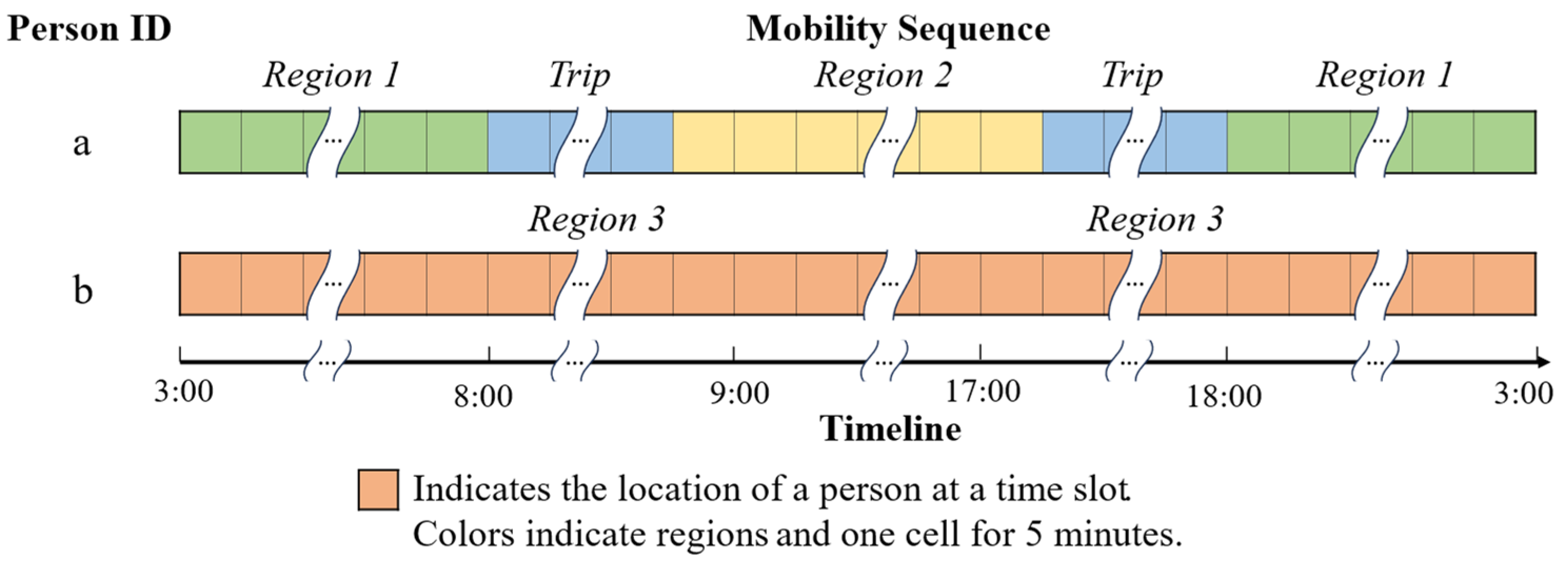
3.2. Construction of Daily Mobility Sequences

The whole survey area is divided into 342 regions for 2008 (as shown in Figure 2), and the division is kept the same for other years. These regions are the spatial units for people’s locations. Regions outside the survey area are treated as another region. A day is segmented into 288 slots (5 min for each slot), and for each person, we assign each slot as the person’s location during that 5-minute interval. If the person was traveling during the interval, the slot is assigned as “Trip”. In this manner, one mobility sequence is constructed for one person with a length of 288. Figure 3 shows two examples of mobility sequences. In the original datasets, 0.79% of stays and 4.69% of trips last for less than 5 min, and they are at the risk of being ignored. On the other hand, increasing the temporal granularity increases the computation time significantly. Considering the above, the length of the slot is set to be 5 min.

3.3. Spatial Datasets and Data Preprocessing

Two additional datasets, namely, the Land Use Mesh data (the dataset is publicly available at: https://nlftp.mlit.go.jp/ksj/gml/datalist/KsjTmplt-L03-b-v3_1.html (accessed on 5 April 2023)) and Land Price data (the dataset is publicly available at: https://nlftp.mlit.go.jp/ksj/gml/datalist/KsjTmplt-L01-v3_1.html (accessed on 5 April 2023)), are used. For the first dataset, the map is divided into 100 m × 100 m cells, and the land use type is provided for each cell.

Table 2. Details of land use types.

Land Use Type	Subtype	Description
Farm and forest	Farmland	Wet, dry, swampy lotus fields and rice fields.
	Other farmland	The land used for growing wheat, upland rice, vegetables, grassland, etc.
	Forest	The land densely populated with perennial vegetation.
Empty	Empty	Wastelands or land with cliffs, rocks, perennial snow, etc.
Building	Buildings	Residential or urban areas where buildings are densely built up.
	Other constructions	The land for an athletic field, airport, baseball field, school, harbor area, etc.
Road	Road	Road or railway.
Water	River and lake	Artificial lakes, natural lakes, ponds, fish farms, etc.
	Waterfront	Areas of sand, rubble, and rock bordering the beach.
	Sea area	Including hidden rocks and mudflats in the sea.

shows the five classes of land uses and their details. Neighborhood characteristics have effects on individual travel behaviors, while forests and rivers that are far away from residential areas may have little impact on people’s mobility patterns. Thus, when preparing the land use for each region, cells within one kilometer of the constructed areas (the “Building” type in Table 2) are taken into account. Using the second dataset, prices per square meter for a large number of houses are available. The land value is further normalized so that the average value over all regions is one for each year to eliminate the effect of inflation over the years. From the two datasets, we obtained the proportions of land use types and the average land value for residential houses in each region. In addition to land use and land value, three other factors are taken into account. Using the PT data, the average family size (i.e., the number of people in a family) is aggregated for each region; integrating person trip survey data and the land use data, population density in the constructed area (the “Building” type in Table 2) for each region is calculated. Following previous studies [5,29], people are classified into four groups based on their age and occupation: workers and colleague students, household wives/husbands and the unemployed, high school students, and children under fifteen years old. The proportion of each age–occupation group in each region is aggregated.

To summarize, five feature values are prepared for each region: (1) the proportions of land use types, as listed in Table 2, (2) average family size, (3) population density, (4) average land value, and (5) the proportions of people in different age–occupation groups. The five regional characteristics may have important impacts on daily mobility. First, land use and family structure have been shown to have critical impacts on mobility patterns, and they are reflected by the first two factors. Second, population density and land value can be indicators of the accessibility to various facilities, transportation services, and the city center. Thus, they may have potential effects on population movements. Third, previous studies [5,29] have revealed that people from different age–occupation groups show different activity–travel patterns and their proportions should have impacts on the mobility patterns in a region. For each region, the above statistics are called the contextual factors in the following sections. They are used as inputs in the models for mobility generation/prediction.

4. A Transformer-Based Model for Mobility Generation and Prediction

In this section, we introduce a model that generates/predicts mobility patterns accounting for contextual factors (e.g., land use, land value). The region (i.e., the location) in the mobility sequences is a categorical variable, and when transformer models or RNN models (such as LSTM) are applied, it should be embedded into a numerical vector. In other words, regions should be converted into vectors representing the information from the regions. They are key components for transformer models. When there is only one scenario (one-year data in this study), the conversion can be performed with conventional embedding methods, and the vector representations are fixed. In our case, as contextual factors of any region have varied over the years, the vector representing a target region should vary with contextual factors, not only those of the target region but also those of other regions, either close or far away. This characteristic enables the constructed model to predict the mobility patterns in a new scenario, responsive to the changes in contextual factors in any region. After regions are embedded, conventional generation architectures can be applied.

To convert a region (categorical variable) and its contextual factors (numerical variables) into a vector, the self-attention mechanism is applied. As an important part of the transformer model, the self-attention mechanism identifies the importance of different elements on the target element and outputs a comprehensive feature for the target element. It captures the relationship between elements (i.e., regions in this study) and thus is suitable for our conversion task. After regions are represented by vectors, the conventional Generative Pre-trained Transformer model (commonly called the GPT model) takes such vectors as input and generates/predicts mobility patterns. Here, a masked self-attention mechanism is integrated using the GPT model. The framework of the model is illustrated in Figure 4. It includes one self-attention part for embedding (i.e., for the conversion from regions and factors to vectors) and one GPT model (i.e., for the generation of mobility sequences). The two parts are connected, and the parameters of them are trained together.

Compared with other deep learning approaches (e.g., RNN), the proposed framework has several advantages. First of all, most deep learning approaches (including the one proposed in this paper) synthesize mobility sequences by predicting locations one by one. In other words, the i-th location (i.e., location at the i-th time slot) is predicted based on previous locations from the first to the i−1-th. Information from vector representations of previous locations is the input to predict the next location. In our model, the vector representation of any region (location) is created considering regional attributes from all other regions using the self-attention embedding module. Thus, the prediction of the next location is responsive to not only the regional factors of the previous regions but also any region in the study area. On the other hand, most existing models do not have such a feature, where the next location is predicted based on only regional features of previous locations. Second, the GPT model enables us to understand how the predictions are made to a certain level, as shown in Section 5.4.2. The two components of the model are detailed in the next two subsections.

4.1. The Self-Attention Mechanism for Embedding

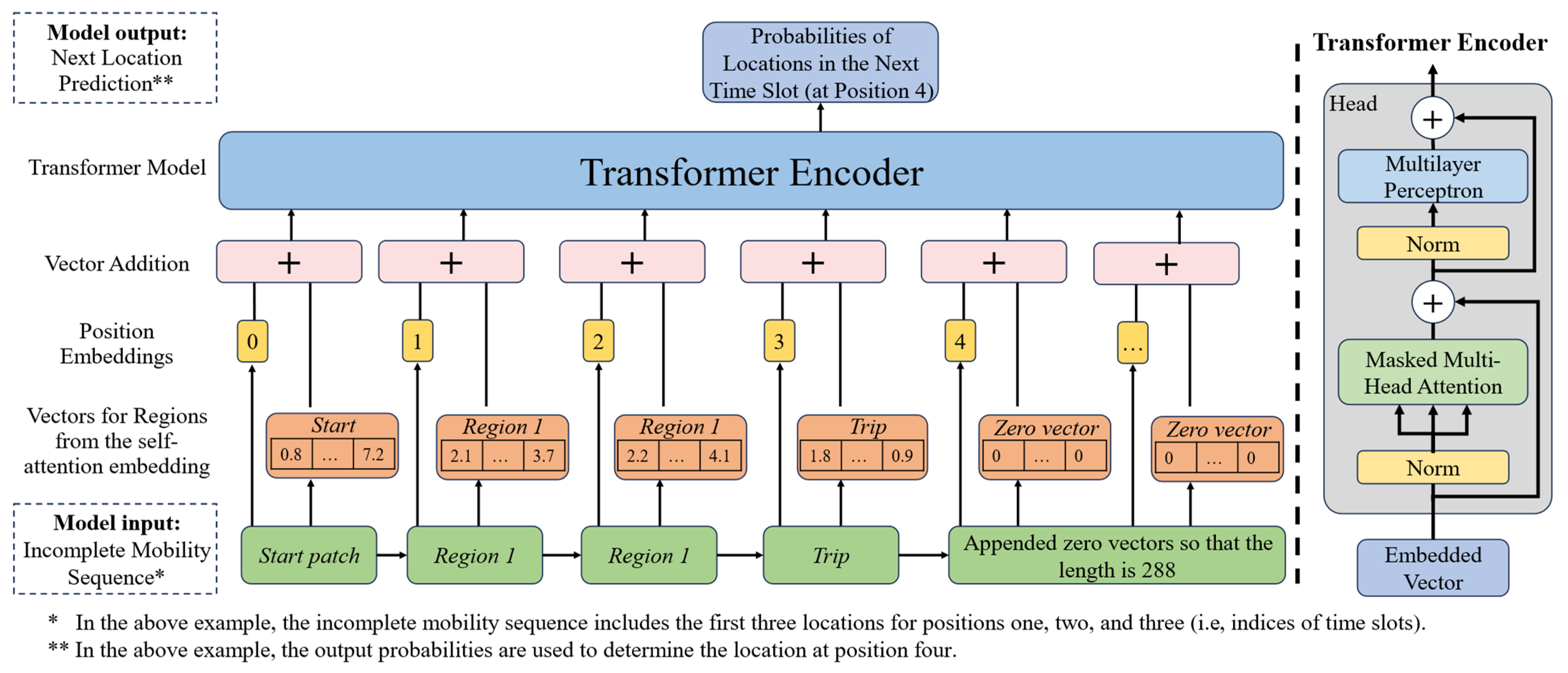
For any year $y$, the self-attention mechanism uses three matrices: $Q_y$, $K_y$, and $V_y$. They are commonly named queries, keys, and values. In the following, we will introduce how $Q_y$ is constructed from regional features. For $K_y$ and $V_y$, the construction methods are basically the same. In the following equations, capital letters indicate matrices, while lowercase letters indicate vectors.

Region is a categorical variable (regions are represented by region ID), and any region has numerical features (i.e., contextual factors) that vary over the years. For any region $i$ ($i=1,2,\dots$), we denote its numerical features in year $y$ as $x_{i,y}$. The self-attention module first converts the categorical variable and the numerical features into two vectors of the same length, $d$:

$$q_{c,i}=E_{c,Q}\left(i\right),E_{c,Q}\in {\mathbb{R}}^{n\times d},q_{c,i}\in {\mathbb{R}}^{1\times d}$$

(1)

$$q_{f,i,y}=x_{i,y}{E}_{f,Q},x_{i,y}\in {\mathbb{R}}^{1\times l},E_{f,Q}\in {\mathbb{R}}^{l\times d},q_{f,i,y}\in {\mathbb{R}}^{1\times d}$$

(2)

where $E_{c,Q}\left(i\right)$ is the $i$-th element of the region-embedding matrix, which is a vector (i.e., $q_{c,i}$) of length $d$ representing the categorical variable for region $i$; $n$ is the number of regions; $x_{i,y}$ is the numerical feature of length $l$; and $E_{f,Q}$ is a 2-D matrix of size $l\times d$, which projects $x_{i,y}$ into a vector of length $d$. $E_{c,Q}$ and $E_{f,Q}$ are parameters that will be learned for constructing queries (i.e., $Q$). $q_{c,i}$ and $q_{f,i,y}$ are then added into a vector:

$$q_{i,y}=q_{c,i}+q_{f,i,y},q_{i,y}\in {\mathbb{R}}^{1\times d}$$

(3)

where $q_{i,y}$ is called the “query” element in the self-attention mechanism. For $n$ regions, the query elements are stacked together to form the queries, $Q_y$, a 2-D matrix of size $n\times d$. Using the same procedure, but replacing ($E_{c,Q}$, $E_{f,Q}$) with ($E_{c,K}$, $E_{f,K}$) and ($E_{c,V}$, $E_{f,V}$), we obtain the “keys” matrix, $K_y$, and the “values” matrix, $V_y$, for the self-attention mechanism. Ideally, we want $E_{c,Q}$, $E_{c,K}$, and $E_{c,V}$ to account for regional characteristics that are not included in the contextual factors, such as some regional-specific conventions or correlations that do not vary over the years. $E_{f,Q}$, $E_{f,K}$, and $E_{f,V}$ are intended to account for numerical (i.e., contextual) factors input into the model. Using $Q_y$, $K_y$, and $V_y$, the self-attention model then outputs the vector matrix representing all regions:

$$R_y=\mathrm{s}\mathrm{o}\mathrm{f}\mathrm{t}\mathrm{m}\mathrm{a}\mathrm{x}\left(\frac{Q_y{K}_y^T}{\sqrt{d}}\right)V_y,Q_y,K_y,V_y\in {\mathbb{R}}^{n\times d},R_y\in {\mathbb{R}}^{n\times d}$$

(4)

where $R_y$ is a matrix of size $n\times d$, and each row is a vector representing a region, which varies with the contextual factors of all regions. In addition, regions outside the survey area are treated as one region and its contextual factors in a certain year are set to the average value of contextual factors of all regions in the year. Travel behavior (“Trip”) is treated as a region. Its contextual factor is set to be a zero vector. Since travel behavior may have a relationship with regional attributes in a year, it is processed in the same manner as regions, and its vector representation is included in $R_y$. Moreover, when generating mobility sequences, there is a start patch according to which the first location is generated. The start patch is also treated as a region class. Since the probability of the first location should vary with the features of different regions, the representation vector of the start patch is also calculated using the above procedure. Its contextual factor is set to be a zero vector of length $d$, and the final vector representation is also one row in $R_y$. In conclusion, there are 345 region vectors in $R_y$ (i.e., $n$ = 345), including 342 vectors for regions in Figure 2, one vector for regions outside the survey area, one for the travel behavior, and one for the start patch.

The matrix $R_y$ can be used as the vector representation of regions, the travel behavior, and the start patch. To include more complicated patterns, in our study, $R_y$ is further linearly projected twice, and the final projected matrix (also of size $n\times d$) is the matrix representing regions, travel, and the start patch. In addition, the dimension of value elements (that form $V_y$) can be different from that of the query/key elements (that form $Q_y$ and $K_y$). For simplicity, we use the same dimension (i.e., $d$) for all of them.

Moreover, the self-attention model could include multiple “patterns” of relationships between regions by generating multiple $R_y$ matrices using different parameter settings of ($E_{c,Q}$, $E_{f,Q}$), ($E_{c,K}$, $E_{f,K}$), and ($E_{c,V}$, $E_{f,V}$). The $R_y$ matrices could be concatenated to a 2-D matrix of size $n\times \left(hd\right)$, where the number of parameter settings (patterns) is $h$.

4.2. The GPT Model

When the vector representations of regions are obtained, we apply the conventional GPT model for mobility generation. Figure 5 shows the architecture of the GPT model. For an incomplete mobility sequence of length $m$, the vector representations of its regions (region vectors hereafter) from Section 4.1 are prepared first. Second, the positions of regions ($1,2,\dots ,288$) on the sequence (i.e., time) are embedded into vectors of length $d$ (position vector hereafter), the same as the length of region vectors. The position vectors and region vectors are added (“Vector Addition” in Figure 5), creating $m$ vectors of length $d$. The series of vectors is appended with zero vectors so that there are 288 vectors of length $d$ (if the start patch is included, there are 289 vectors). They are the standard input into the transformer model (“Transformer Encoder” in Figure 5), which outputs the probability of the location at the next time slot (i.e., the $m+1$ slot). The structure of the transformer encoder is on the right-hand side. Interested readers may refer to the work by Vaswani et al. (2017) [30] for more details on the transformer model and the self-attention mechanism. When generating mobility sequences, the start patch is input into the model, and the probabilities of locations at time one are calculated. The first location is randomly selected based on the probabilities. The start patch and the first location are then input into the model, and the probabilities of the next locations are the outputs. After random selection on the second location, the start patch and the two locations are input into the model. By iterating the above steps 288 times, one mobility sequence is constructed, and more can be generated using the same procedure.

The grey block in Figure 5 is also called a head. It can be duplicated in parallel, as well as stacked, multiple times to increase the complexity of the model. The number of parallel duplication of heads is the same as the number of parameter settings (i.e., $h$) in Section 4.1, and different heads receive different vector representations of regions ($R_y$ matrix) and position vectors. The number of layers of heads (stack) is denoted by $L$ hereafter. $h$, $L$, and $d$ are three hyperparameters that determine the complexity of the model.

5. Experiments and Results

The model is trained using datasets from 1978 to 1998. Datasets are generated for 1978, 1988, 1998, and 2008 with different contextual factors for different years. The generative power of the model is evaluated by comparing the similarities between the real and generated datasets from 1978 to 1998. Generation results for 2008 are examined for the prediction power of the model because the 2008 data are not used during the training.

5.1. Setup and Evaluation Metrics

The five factors for each region mentioned in Section 3.3 are concatenated into a vector of length $l$ and serve as the input to the self-attention model for region embedding. The three hyperparameters, $h$, $L$, and $d$, are set to be 3, 3, and 24, respectively (i.e., three heads, three layers, and twenty-four dimensional vectors for queries, keys, and values). These hyperparameters are set with multiple experiments so that the increase in them does not lead to significant improvements in terms of the generation results. The model is trained until the loss is small enough and additional training does not improve the model performance on the training dataset (i.e., the 1978–1998 data).

To evaluate the mode performance, we also apply an LSTM-based model to generate and predict mobility data. As stated in Section 2.2, the LSTM model is one of the widely adopted frameworks for mobility generation. However, most existing models for mobility synthetization do not consider contextual factors and thus cannot be used for mobility prediction given different scenarios (i.e., different settings of contextual factors). To make a fair comparison, the vector representation for a region used in the LSTM-based model is created using the contextual factors of this region (using a linear transformation) and a categorical embedding. This enables the LSTM model to predict mobility patterns for new cases. The dimension of vector representations of regions, which is also the number of input features of the LSTM model, and the number of features in the hidden state of the LSTM model are set to 64. The number of recurrent layers in the LSTM model is set to 3. Our multiple experiments indicate that larger LSTM models show slightly better performance on the training datasets but worse performance in predicting the 2008 mobility. Thus, larger models are not used.

In line with existing studies, three aggregate statistics are used to evaluate the generation accuracy: the distribution of the number of trips, the distribution of the number of distinct regions visited, and the distribution of travel time for travelers. However, these three measurements can be insufficient. Even if aggregated statistics are perfectly synthesized, the generated datasets could be potentially very different from the original ones. Following Wang and Osaragi (2022) [5], the sequential characteristics are evaluated for the generated datasets. Sequential characteristics indicate which regions are traveled by people in which order, which is evaluated by counting the number of distinct region sequences. A region sequence is similar to a mobility sequence, as defined in Section 3.2, but the duration of stays and trips are ignored. For instance, the two examples in Figure 3 are converted to be the two region sequences: (1) $region1\to trip\to region2\to trip\to region1$ and (2) $region3$. For the first sequence, the start times and durations of trips/stays (temporal information) are discarded. Different people may have the same region sequences, and the number of distinct region sequences is counted for the real and the generated datasets. The count of region sequences is a stricter metric than aggregated statistics. A region sequence generally has fewer counts if it includes more trips, and the counts of sequences may vary for several orders of magnitude. Thus, it is improper to plot all the distinct region sequences on the same plot. We classify them into three types: region sequences with no trip (i.e., people stay in the same location for the whole day, Type 1 hereafter), region sequences with two trips whose start regions are the same as end regions (Type 2), and other region sequences (Type 3). The results are compared separately.

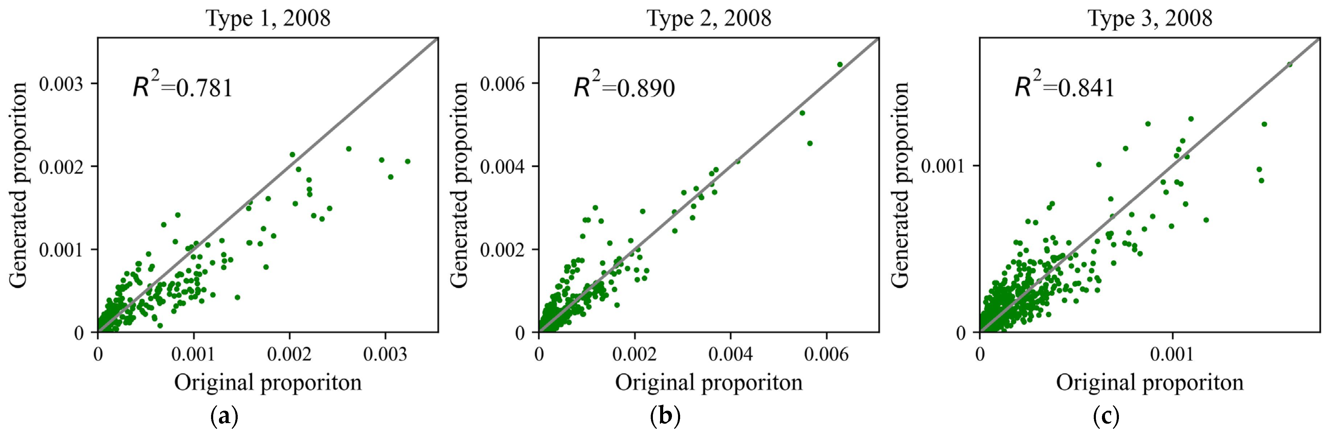
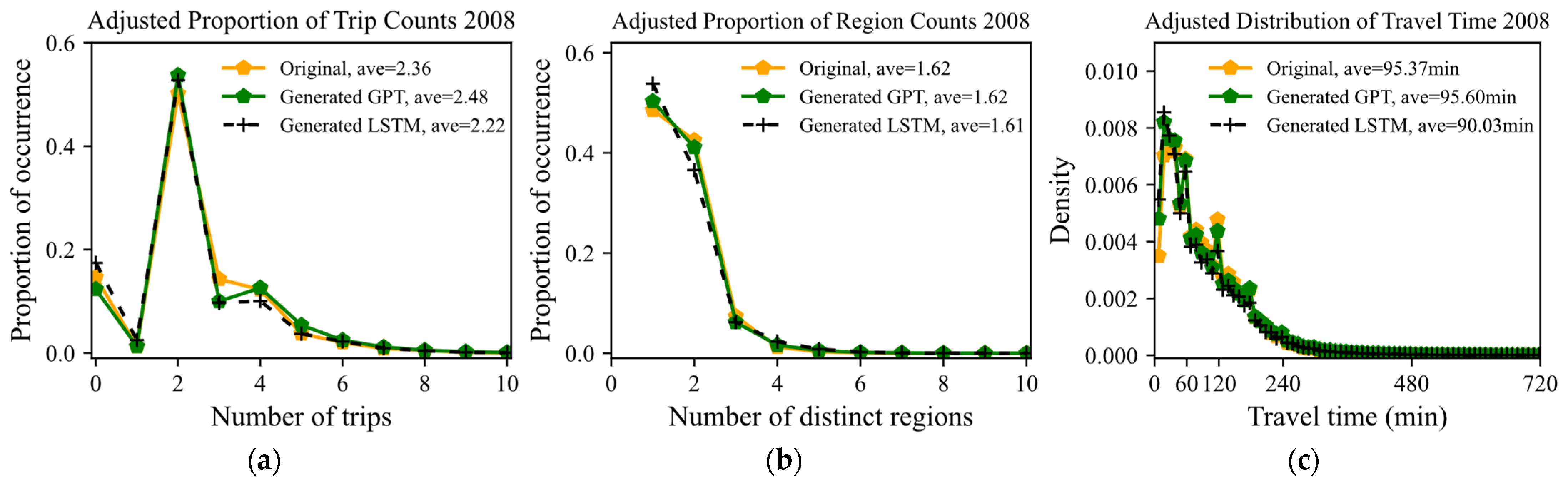
5.2. Evaluation of the Generation Power

Generation power is examined by comparing the real and generated mobilities for 1978, 1988, and 1998. Figure 6 shows the aggregated statistics for the original datasets and the generated datasets using the transformer-based (GPT in Figure 6) and the LSTM-based (LSTM in Figure 6) models. Figure 7 shows the sequential evaluation (i.e., comparison of the real and generated region sequences) for 1978–1998 for the transformer-based model. To save space, the same evaluation for the LSTM-based model is shown in Appendix A (Figure A1).

Regarding the distribution of trip counts (i.e., figures at the top of Figure 6), the generated results are good for both models. The proportion of people with four trips is underestimated by a tiny amount using the transformer-based model, while that of two trips is undervalued using the LSTM model. The average values reproduced with the transformer model are slightly more accurate than the LSTM model. Overall, the distribution of the number of trips seems to be stable from 1978 to 1998. In terms of the distribution of the number of distinct regions visited (figures in the middle), the transformer model seems to outperform the LSTM model. From 1978 to 1998, the percentage of individuals who visited only one location dropped from 60% to 55%, while that of people who visited two locations increased from 33% to 39%. Consequently, the average number of regions visited ascended from 1.50 to 1.54. This variation is captured with the transformer model. On the other hand, the LSTM model does not seem to have learned the differences precisely, as evidenced by the unvarying generations of distributions and average values over the years. The distribution of travel time for travelers (figures at the bottom) varied over time. Short-time daily travel declined, and the average daily travel time rose. The distribution of travel time is replicated using the two models, while the transformer-based makes a better prediction of the average values than the LSTM-based model. In terms of the sequential evaluation in Figure 7, it can be observed that all types of region sequences are well-reproduced, especially for Type 1 and Type 2. These observations suggest that the generation power of the transformer-based model is satisfactory. The comparison of $R^2$ values in Figure 7 and Figure A1 indicates that the transformer-based model outperforms the LSTM-based model.

5.3. Evaluation of the Prediction Power

Figure 8 (for the two models) and Figure 9 (for the transformer model) show the aggregated distribution of three measurements and the sequential evaluation for 2008. The sequential evaluation for the LSTM-based model for 2008 is shown in Figure A2 in Appendix A. At first glance, the generation of aggregated statistics (Figure 8) is not bad. In terms of the sequential evaluation (Figure 9 and Figure A2), compared with those in Figure 7 and Figure A1, there are significant differences between the real and generated region sequences, especially for Type 1 and Type 2 sequences.

From the sequential evaluation, the difference between the real and generated datasets is remarkable. This suggests that the two models are not capable of predicting what regions are traveled by people in what order. Thus, the estimated Origin–Destination matrix using such data can be significantly different from reality. A further analysis shows that the proportions of people being in different regions at the start time (3:00 a.m.) are different from the real data. In other words, the probabilities for locations at time one are incorrectly predicted when the start patch is input into the model. If we knew the start location of people (at 3:00 a.m.), better predictions could have been made. Researchers have developed various models to predict the distribution of the nighttime population with high accuracy, and such information could be one of the scenario settings for mobility prediction. Given the nighttime population (i.e., the distribution of people at 3:00 a.m.), the generated mobility data can be modified. We assign each mobility sequence a weight such that the proportions of people in different regions at time one agree with the real data. For a mobility sequence $s$, the weight assigned to it is:

$$w\left(s\right)=\frac{M_{s\left(1\right)}/M}{M_{s\left(1\right)}^{\prime }/M^{\prime }}$$

(5)

where $w\left(s\right)$ is the weight assigned to sequence $s$; $s\left(1\right)$ is the first location of sequences $s$; $M_{s\left(1\right)}$ is the number of original sequences whose first location is $s\left(1\right)$; $M$ is the total number of original sequences; $M_{s\left(1\right)}^{\prime }$ is the number of generated sequences whose first location is $s\left(1\right)$; and $M^{\prime }$ is the total number of generated sequences. Sequences with the same start location are assigned the same weight. This operation is equivalent to specifying the probabilities of the regions at time one (i.e., the output probabilities when the start patch is the input) and generates mobility sequences accordingly. The evaluations of weighted mobility sequences are shown in Figure 10, Figure 11 (for the transformer-based model), and Figure A3 (in Appendix A for the LTSM-based model). For the sequential evaluation (Figure 11 and Figure A3), the accuracy is visually improved, and the transformer model performs better.

Noticeably, the proportion of people who visited one distinct region dropped (60%, 56%, 55%, and 49% for 1978, 1988, 1998, and 2008, respectively) and those who visited two regions increased (33%, 37%, 39%, and 43% for 1978, 1988, 1998, and 2008). The variations from 1978 to 2008 are significant. The transformer-based model synthetizes these attributes accurately, while the outputs of the LSTM-based model do not change much with contextual factors. The transformer model also performs better in terms of the generated distribution of travel time, especially the predicted average value for 2008 (Figure 10c). The sequential evaluations ($R^2$ values in Figure 11 and Figure A3) further validate its superiority. Such observations suggest that the transformer model has captured some essential relationships between inputs and outputs while the LSTM model has not. However, the reasons why the transformer-based model outperforms the LSTM-based model are not yet apparent. From Figure 6 and Figure 10, it can be observed that the average number of trips is stable over the years, while the average number of regions visited and the average travel time increased. This implies that the average trip distance has increased, probably due to the development of transportation services and the change in urban structures (related to urban land use and land value). One of the possible theories explaining the superior performance of the transformer model is that people’s travel behaviors originating from one region are not only related to the characteristics of the region but also to other regions nearby or even far away, as they can be potential destinations. The proposed transformer-based model captures such relationships with self-attention embedding and thus makes accurate predictions.

Despite the prediction accuracy, it is still in question if the transformer-based model has learned enough to predict mobility patterns given a new scenario. For the number of trips in Figure 10a, the proportion of people with three trips is underestimated. The generated distribution of trip counts for 2008 looks similar to those in 1978–1998, suggesting that the model made limited responses to the contextual factors in 2008. For distinct regions visited in Figure 10b, the pattern generated with the transformer model looks similar to the real pattern in 2008 and different from patterns in other years. This suggests that the model made an accurate extrapolation for the number of regions visited based on the contextual factors. For the distribution of travel time, the generated pattern is similar to that in 1998, and short daily travel times are overestimated. More datasets are needed to validate the prediction power.

5.4. Interpretation of the Transformer Model

In this subsection, we provide a deeper analysis of what the model has learned. Specifically, the spatial similarity and temporal relationship of daily mobility are evaluated.

5.4.1. Spatial Similarity of Regions

Vector representations for regions imply the meaning of regions (locations) for human daily mobility. We would expect that regions that are close, or regions that have similar accessibility to various facilities, should be represented similarly. We select nine regions, four from the city center (Chuo-ku, Tokyo; Chuo-ku, Chiba; Nishi-ku, Kanagawa; and Arakawa-ku, Tokyo) and five from the suburban areas (Hachioji, Tokyo; Tsukuba, Ibaraki; Oi-machi, Kanagawa; Hanyu-shi, Saitama; andAsahi-shi, Chiba) to analyze what was learned by the model. The $R_y$ matrices in Equation (4) are concatenated into a 2-D matrix of size $n\times \left(hd\right)$. For any of the selected regions, the cosine similarities between the vector representations (i.e., rows of the 2-D matrix) of the target region and other regions are calculated and visualized on the map for 1998. The results are shown in Figure 12. It can be observed that the vector representations of regions are similar to those of regions that are close to them. For a suburban region, its vector representation can be similar to those of other suburban regions, even if they are far away.

Using principal component analysis, vector representations are visualized in the 2-D space with the first two principal components (Figure 13). The colors indicate the distance between the region and the city center (the Tokyo Station). It is observed that regions close to the city center are on the right side and those far from the center are on the left. On the other hand, regions on the upper side are mostly on the east, while the lower side contains more on the west. Visually, regions seem to be evenly distributed, and no significant clusters are observed. This may imply that human mobilities in different regions mostly vary smoothly. The analyses of Figure 12 and Figure 13 suggest that the model learned the spatial structure of regions, which generally agrees with our common sense.

5.4.2. Temporal Relationship of Daily Mobility

The self-attention mechanism in the GPT model enables us to explore the relationship between the current location and previous locations by analyzing the attention matrix. Using a conceptually similar approach as [31], we examine the temporal relationship among people’s locations. Suppose that the input into the GPT model (after “Vector Addition” in Figure 5) is a sequence of vectors $Z_s\in {\mathbb{R}}^{N\times d}$, where $N$ is the number of vectors (equal to 289 in this study including the start patch) and $s$ indicates the sequence. In the transformer encoder (“Transformer Encoder” in Figure 5), $Z_s$ is projected to three matrices of size $N\times d$, namely, $Q_s$, $K_s$, and $V_s$:

$$\left[Q_s,K_s,V_s\right]=Z_{s}U,U\in {\mathbb{R}}^{d\times 3d},Q_s,K_s,V_S\in {\mathbb{R}}^{N\times d}$$

(6)

The attention matrix is:

$$A_s=\mathrm{s}\mathrm{o}\mathrm{f}\mathrm{t}\mathrm{m}\mathrm{a}\mathrm{x}\left(\mathrm{m}\mathrm{a}\mathrm{s}\mathrm{k}\left(\frac{Q_s{K}_s^T}{\sqrt{d}}\right)\right),Q_s,K_s\in {\mathbb{R}}^{N\times d}$$

(7)

The $i$-th row of $A_s$ indicates the “attention” paid to previous locations to predict the $i+1$-th location on sequence $s$. It indicates the weights of previous locations to predict the next location. The higher the value, the more attention is paid. For multi-head and multi-layer self-attention models, there is one attention matrix for each head on each layer. These attention matrices are summed into one matrix for the simplicity of interpretation. Since attention can be only paid to previous locations and the sum of attention values equals one in each row of $A_s$, locations early in the day have fewer previous locations and thus more attention (weights) to each of the previous locations. For a fair comparison, each row is weighted with the average attention (value) for previous locations. Figure 14 shows the average weighted attention matrix for randomly selected 10,000 mobility sequences. Attention is usually paid to locations that are temporarily nearby, as the values are higher near the diagonal. This might be because people are likely to stay in the same place for consecutive time slots, and thus the current location is powerful in predicting the next location. To predict locations from 8:00 to 15:00, the location around 4:30 and the locations after 8:00 are paid the most attention. Locations at night (after 18:00) are mostly predicted by the location around 4:30 and locations after 15:00. The model paid little attention to locations in the morning (from 6:00 to 12:00) when predicting night locations, probably indicating the weak correlation between them. It should be noted that low attention values to some time slots do not always imply low temporal correlations between the target and these slots—it only suggests that the model made the prediction based on little information from these slots. We expect that the model should generally pay more attention to time slots with high temporal correlations, but not necessarily.

Vector representations of time slots (i.e., position vectors) are input into the model to predict future locations. When making predictions for the next location, much of the attention is paid to previous time slots that are nearby. If two time slots are represented by similar vectors (position vectors), we would expect that their following locations might be similar (but not necessarily). To justify that the model has learned something reasonable, the temporal similarity in daily mobility is examined by investigating the vector representations of time slots (i.e., the position vector). Figure 15 shows the cosine similarities between position embeddings. The vector representations for time slots nearby are similar, probably suggesting their consecutive locations are similar. This agrees with the fact that most stay last for more than one time slot. The embeddings at nighttime (from 21:00 to 6:00) are similar to each other, indicating that people’s locations after these slots (perhaps several slots later than them) are likely to be the same. Visually, there seem to be several time blocks that have higher similarities for time slots within them (black boxes in Figure 15): 6:00 to 8:00, 9:00 to 12:00, 13:00 to 17:00, and 18:00 to 24:00. Their consecutive slots are likely to correspond to the daily time before work/school in the morning, during morning work/school, during afternoon work/school, and in the evening. The high embedding similarity suggests that people are likely to be at the same location during these periods. In addition, vectors for time slots from 7:00 to 9:00 are similar to those even for slots in the afternoon, suggesting that destinations for morning trips are likely to be the same for the location during the daytime. The above analysis provides intuition about what might have been learned by the model, which mostly agrees with our experience. Since we cannot yet fully understand the transformer model and the model may not capture everything correctly, the above inferences should be validated with other statistical methods.

6. Discussion and Conclusions

In this paper, we applied the transformer-based model to learn human daily mobilities using 1978–1998 data. The model includes one self-attention mechanism to output vector representations for regions and one GPT model that takes these vectors as input and outputs daily mobility patterns. The performance of the model is evaluated using aggregated statistics (i.e., the distribution of the number of trips, distinct regions visited, and travel time) and sequential characteristics. Our evaluations indicate that the generation and prediction powers of the model are satisfactory and superior to an LSTM-based model. Analyses of the results for 1978–1998 suggest that the model generated daily mobility with high accuracy. Regarding the prediction for 2008, the three aggregated measurements are well reproduced, but the sequential characteristics are different from the real data. After applying weights to mobility sequences so that the generated number of people in each area at nighttime (i.e., 3:00 a.m.) agrees with the real data, significant improvements are observed in terms of sequential characteristics. This observation suggests that if the start location could be correctly predicted, higher prediction accuracy would be achieved. This also implies that the vector representation of the start patch is not well-learned, and perhaps more contextual factors or other learning algorithms should be used. In addition, the predicted frequency of trips and the distribution of travel time for 2008 look similar to those from the training data, while the distribution of distinct regions visited is well-reproduced for 2008 and is different from other years. This indicates that the model made some reasonable predictions based on the contextual factors, but not comprehensively. It is worth noting that the model was trained using only 3-year data (three contextual factor settings), and its full prediction power may not be unlocked due to the limitation of datasets. If more datasets were available, the prediction accuracy could be improved, and deeper evaluations could be made.

Moreover, by evaluating the vector representations of regions and positions (i.e., time slots), the spatial structures of regions, as well as the temporal relationship of mobility, seem to have been learned by the transformer model. The learned structure basically agrees with our common sense. Interpretations from the self-attention mechanism are unique to the transformer model, and further analyses can be conducted using other formations of the model. This suggests the promising potential of using the model for mobility modeling and probably knowledge extraction.

Previous studies have used various deep learning frameworks to generate human mobility patterns, and synthetic datasets were mostly evaluated with several aggregate statistics. Our study shows that aggregated statistics can be limited. For example, three aggregate measurements are well reproduced for the 2008 data (Figure 8) while the sequential features (at a “more disaggregate level”) can be remarkably different from reality (Figure 9) if the weighting procedure is not applied. On the other hand, the accurate synthetization of sequential characteristics could be critical when constructing the Origin–Destination matrix for traffic analysis. This work shows that, when mobility data are generated and evaluated, metrics that reveal more detailed spatial–temporal characteristics could be helpful for a comprehensive evaluation.

There are several future topics for this study. First of all, one of the purposes of generating synthetic data is to share mobility data while protecting individual privacy. Although the generation power is high, there is still a question of to what extent privacy is protected. This will be examined in future studies. Second, since there are only three years of data for training the model, the learning ability cannot be investigated comprehensively. If sufficient data are available, a universal model might be constructed for mobility generation and prediction under a wide range of scenario settings.

References

1. Kapp, A.; Hansmeyer, J.; Mihaljević, H. Generative Models for Synthetic Urban Mobility Data: A Systematic Literature Review. ACM Comput. Surv. 2023, 56, 93:1–93:37. [Google Scholar] [CrossRef]
2. Ahmed, B. The Traditional Four Steps Transportation Modeling Using a Simplified Transport Network: A Case Study of Dhaka City, Bangladesh. Int. J. Adv. Sci. Eng. Technol. Res. 2012, 1, 19–40. [Google Scholar]
3. Mladenovic, M.; Trifunovic, A. The Shortcomings of the Conventional Four Step Travel Demand Forecasting Process. J. Road Traffic Eng. 2014, 60, 5–12. [Google Scholar]
4. Mo, B.; Zhao, Z.; Koutsopoulos, H.N.; Zhao, J. Individual Mobility Prediction: An Interpretable Activity-Based Hidden Markov Approach. arXiv 2021, arXiv:2101.03996. [Google Scholar]
5. Wang, W.; Osaragi, T. Daily Human Mobility: A Reproduction Model and Insights from the Energy Concept. ISPRS Int. J. Geo-Inf. 2022, 11, 219. [Google Scholar] [CrossRef]
6. Rasouli, S.; Timmermans, H. Activity-Based Models of Travel Demand: Promises, Progress and Prospects. Int. J. Urban Sci. 2014, 18, 31–60. [Google Scholar] [CrossRef]
7. Bhat, C.R.; Guo, J.Y.; Srinivasan, S.; Sivakumar, A. Comprehensive Econometric Microsimulator for Daily Activity-Travel Patterns. Transp. Res. Rec. 2004, 1894, 57–66. [Google Scholar] [CrossRef]
8. Nurul Habib, K.; El-Assi, W.; Hasnine, M.S.; Lamers, J. Daily Activity-Travel Scheduling Behaviour of Non-Workers in the National Capital Region (NCR) of Canada. Transp. Res. Part A Policy Pract. 2017, 97, 1–16. [Google Scholar] [CrossRef]
9. Liu, P.; Liao, F.; Huang, H.-J.; Timmermans, H. Dynamic Activity-Travel Assignment in Multi-State Supernetworks under Transport and Location Capacity Constraints. Transp. A Transp. Sci. 2016, 12, 572–590. [Google Scholar] [CrossRef]
10. Miller, E.J.; Roorda, M.J. Prototype Model of Household Activity-Travel Scheduling. Transp. Res. Rec. 2003, 1831, 114–121. [Google Scholar] [CrossRef]
11. Drchal, J.; Čertický, M.; Jakob, M. Data-Driven Activity Scheduler for Agent-Based Mobility Models. Transp. Res. Part C Emerg. Technol. 2019, 98, 370–390. [Google Scholar] [CrossRef]
12. Allahviranloo, M.; Recker, W. Daily Activity Pattern Recognition by Using Support Vector Machines with Multiple Classes. Transp. Res. Part B Methodol. 2013, 58, 16–43. [Google Scholar] [CrossRef]
13. Hesam Hafezi, M.; Sultana Daisy, N.; Millward, H.; Liu, L. Framework for Development of the Scheduler for Activities, Locations, and Travel (SALT) Model. Transp. A Transp. Sci. 2022, 18, 248–280. [Google Scholar] [CrossRef]
14. Hafezi, M.H.; Liu, L.; Millward, H. Learning Daily Activity Sequences of Population Groups Using Random Forest Theory. Transp. Res. Rec. 2018, 2672, 194–207. [Google Scholar] [CrossRef]
15. Huang, D.; Song, X.; Fan, Z.; Jiang, R.; Shibasaki, R.; Zhang, Y.; Wang, H.; Kato, Y. A Variational Autoencoder Based Generative Model of Urban Human Mobility. In Proceedings of the 2019 IEEE Conference on Multimedia Information Processing and Retrieval (MIPR), San Jose, CA, USA, 28–30 March 2019; pp. 425–430. [Google Scholar]
16. Sakuma, Y.; Tran, T.P.; Iwai, T.; Nishikawa, A.; Nishi, H. Trajectory Anonymization through Laplace Noise Addition in Latent Space. In Proceedings of the 2021 Ninth International Symposium on Computing and Networking (CANDAR), Matsue, Japan, 23–26 November 2021; pp. 65–73. [Google Scholar]
17. Blanco-Justicia, A.; Jebreel, N.M.; Manjón, J.A.; Domingo-Ferrer, J. Generation of Synthetic Trajectory Microdata from Language Models. In Privacy in Statistical Databases; Domingo-Ferrer, J., Laurent, M., Eds.; Springer International Publishing: Cham, Switzerland, 2022; pp. 172–187. [Google Scholar]
18. Berke, A.; Doorley, R.; Larson, K.; Moro, E. Generating Synthetic Mobility Data for a Realistic Population with RNNs to Improve Utility and Privacy. In Proceedings of the 37th ACM/SIGAPP Symposium on Applied Computing, Virtual Event, 25–29 April 2022; Association for Computing Machinery: New York, NY, USA, 2022; pp. 964–967. [Google Scholar]
19. Badu-Marfo, G.; Farooq, B.; Patterson, Z. Composite Travel Generative Adversarial Networks for Tabular and Sequential Population Synthesis. IEEE Trans. Intell. Transp. Syst. 2022, 23, 17976–17985. [Google Scholar] [CrossRef]
20. Rao, J.; Gao, S.; Kang, Y.; Huang, Q. LSTM-TrajGAN: A Deep Learning Approach to Trajectory Privacy Protection. In Proceedings of the International Conference Geographic Information Science, Seattle, WA, USA, 3–6 November 2020. [Google Scholar]
21. Jiang, W.; Zhao, W.X.; Wang, J.; Jiang, J. Continuous Trajectory Generation Based on Two-Stage GAN. In Proceedings of the Thirty-Seventh AAAI Conference on Artificial Intelligence and Thirty-Fifth Conference on Innovative Applications of Artificial Intelligence and Thirteenth Symposium on Educational Advances in Artificial Intelligence, Washington, DC, USA, 7–14 February 2023; AAAI Press: Washington, DC, USA, 2023; Volume 37, pp. 4374–4382. [Google Scholar]
22. Cao, C.; Li, M. Generating Mobility Trajectories with Retained Data Utility. In Proceedings of the 27th ACM SIGKDD Conference on Knowledge Discovery & Data Mining, Singapore, 14–18 August 2021; Association for Computing Machinery: New York, NY, USA, 2021; pp. 2610–2620. [Google Scholar]
23. Solatorio, A.V. GeoFormer: Predicting Human Mobility Using Generative Pre-Trained Transformer (GPT). In Proceedings of the 1st International Workshop on the Human Mobility Prediction Challenge, Hamburg, Germany, 13 November 2023; pp. 11–15. [Google Scholar]
24. Corrias, R.; Gjoreski, M.; Langheinrich, M. Exploring Transformer and Graph Convolutional Networks for Human Mobility Modeling. Sensors 2023, 23, 4803. [Google Scholar] [CrossRef]
25. Lee, M.; Holme, P. Relating Land Use and Human Intra-City Mobility. PLoS ONE 2015, 10, e0140152. [Google Scholar] [CrossRef]
26. Kim, H.; Sohn, D. The Urban Built Environment and the Mobility of People with Visual Impairments: Analysing the Travel Behaviours Based on Mobile Phone Data. J. Asian Archit. Build. Eng. 2020, 19, 731–741. [Google Scholar] [CrossRef]
27. Lee, B.A.; Oropesa, R.S.; Kanan, J.W. Neighborhood Context and Residential Mobility. Demography 1994, 31, 249–270. [Google Scholar] [CrossRef] [PubMed]
28. Osaragi, T.; Kudo, R. Enhancing the Use of Population Statistics Derived from Mobile Phone Users by Considering Building-Use Dependent Purpose of Stay. In Geospatial Technologies for Local and Regional Development; Kyriakidis, P., Hadjimitsis, D., Skarlatos, D., Mansourian, A., Eds.; Springer International Publishing: Cham, Switzerland, 2020; pp. 185–203. [Google Scholar]
29. Wang, W.; Osaragi, T. Generating and Understanding Human Daily Activity Sequences Using Time-Varying Markov Chain Models. Travel Behav. Soc. 2024, 34, 100711. [Google Scholar] [CrossRef]
30. Vaswani, A.; Shazeer, N.; Parmar, N.; Uszkoreit, J.; Jones, L.; Gomez, A.N.; Kaiser, Ł.; Polosukhin, I. Attention Is All You Need. In Advances in Neural Information Processing Systems; Curran Associates, Inc.: Red Hook, NY, USA, 2017; Volume 30. [Google Scholar]
31. Dosovitskiy, A.; Beyer, L.; Kolesnikov, A.; Weissenborn, D.; Zhai, X.; Unterthiner, T.; Dehghani, M.; Minderer, M.; Heigold, G.; Gelly, S.; et al. An Image Is Worth 16 × 16 Words: Transformers for Image Recognition at Scale. arXiv 2020, arXiv:2010.11929. [Google Scholar]
Figure 1. Examples of trips in Person Trip survey data.
Ijgi 13 00035 g001
Figure 2. Regions surveyed (spatial units) for person trips.
Ijgi 13 00035 g002
Figure 3. Examples of mobility sequences.
Ijgi 13 00035 g003
Figure 4. Overall architecture of the generation model.
Ijgi 13 00035 g004
Figure 5. Architecture of the GPT model.
Ijgi 13 00035 g005
Figure 6. Evaluation of the number of trips (proportion of trip counts), the number of distinct regions visited (proportion of region counts), and travel time for travelers. “ave” in the legend indicates the average value, and the bin size of travel time is 10 min. (a) 1978, (b) 1988, and (c) 1998.
Ijgi 13 00035 g006
Figure 7. Sequential evaluation of three types of region sequences using the transformer-based models. (a) Results for 1978, (b) results for 1988, and (c) results for 1998.
Ijgi 13 00035 g007
Figure 8. Evaluation of aggregated statistics for 2008. (a) The number of trips, (b) the number of distinct regions visited, and (c) travel time for travelers.
Ijgi 13 00035 g008
Figure 9. Sequential evaluation of the three types of region sequences using the transformer-based model for 2008. (a) Type 1 sequences, (b) type 2 sequences, and (c) type 3 sequences.
Ijgi 13 00035 g009
Figure 10. Evaluation of aggregated statistics for 2008 with weighted mobility sequences. (a) The number of trips, (b) the number of distinct regions visited, and (c) travel time for travelers.
Ijgi 13 00035 g010
Figure 11. Sequential evaluation of the three types of region sequences using the transformer-based model for 2008 with weighted mobility sequences. (a) Type 1 sequences, (b) type 2 sequences, and (c) type 3 sequences.
Ijgi 13 00035 g011
Figure 12. Cosine similarity of vector representations between the target region and other regions for 1998. Red pentagons are the target regions and green dots are the centroids of building areas for other regions. (a) Nishi-ku, Kanagawa, (b) Chuo-ku, Tokyo, (c) Chuo-ku, Chiba, (d) Hachioji-shi, Tokyo, (e) Arakawa-ku, Tokyo, (f) Tsukuba-shi, Ibaraki, (g) Oi-machi, Kanagawa, (h) Hanyu-shi, Saitama, and (i) Asahi-shi, Chiba.
Ijgi 13 00035 g012
Figure 13. Visualization of the first two principal components for vector representations for 1998.
Ijgi 13 00035 g013
Figure 14. Average weighted attention to previous locations (x-axis) to predict the next (y-axis).
Ijgi 13 00035 g014
Figure 15. Cosine similarity between position vectors. Four black boxes indicate four time intervals: 6:00 to 8:00, 9:00 to 12:00, 13:00 to 17:00, and 18:00 to 24:00.
Ijgi 13 00035 g015