Optimisation Model for Spatialisation of Population Based on Human Footprint Index Correction

Abstract

The availability of high-precision population distribution data is crucial for urban planning and the optimal allocation of resources. To address the limitations of the random forest model in addressing spatial heterogeneity during population spatialisation and the potential for features to be lost or distorted between scale changes, which can result in excessive spatialisation error, this study proposes an optimised population spatialisation model based on the modification of the Human Footprint Index (HFI). A hierarchical feature coding method is used to reduce cross-scale distribution errors. The Human Footprint Index (HFI) was then constructed by selecting a total of seven characteristic factors in five areas, namely, electricity, land use intensity, built environment, transport accessibility, and the level of economic development, which then corrects random forest predictions. The resulting dataset for Suzhou demonstrates the following: (1) the R² of the HFI-corrected data reaches 92.8%, with an accuracy of 92.3% in medium-density areas, significantly outperforming the single random forest model (81.6%) and WorldPop (69.3%) in overall accuracy; (2) the Pearson correlation coefficient for the HFI-corrected data is 0.96, higher than that of WorldPop (0.94) and RFPop (0.91), further validating the model’s accuracy; and (3) the hierarchical coding method reduces cross-scale errors, improving accuracy by five percentage points.

1. Introduction

Census data serve as an important resource for scholarly research and societal advancement. However, their low spatial and temporal resolution makes it challenging to meet the needs of spatial analyses [1]. By contrast, population spatialisation is capable of providing multi-scale population distribution data, which lends support to a variety of spatial analyses and model applications through integration with spatial ecological, social, and economic data [2]. The fundamental concept of demographic spatialisation is the establishment of correlations between supplementary data and population figures at the level of administrative units, subsequently transferring this information to a grid scale to generate highly accurate population distributions [3,4]. The aforementioned data have a plethora of applications in urban planning, resource allocation, environmental protection, and other fields [5,6,7].

The utilisation of global and regional fine-grained population grid datasets has become a prevalent practice in both research and applications [8]. The most commonly used global datasets include GPW, LandScan, and WorldPop, which provide the basis for global population studies [9,10,11]. In recent years, a series of nationwide population grid datasets have been established in China, following the advancement of census and geographic information technology. For example, Xu Xinliang et al. produced a kilometre grid dataset of the spatial distribution of China’s population [12], while Chen et al. developed the 100 m population raster data of China’s seventh population census [13]. However, these datasets are deficient in terms of spatial resolution and update frequency when dealing with urban areas or areas with high population concentration. This makes it challenging to reflect population dynamics in real time, which in turn limits their applicability in rapidly developing urban environments.

With regard to population spatialisation methods, traditional techniques such as area weighting [14] and spatial interpolation [15] are subject to constraints. The current state of the art has facilitated the widespread realisation of population spatialisation across disciplines, with theoretical approaches from a number of disciplines, including demography, geography, economics, urban planning, and environmental science, being integrated. Researchers have introduced multi-source data, such as nighttime lighting, land use, points of interest (POI), and so forth, in conjunction with models such as multiple regression, random forest, and integrated learning, with the objective of enhancing the accuracy of population spatialisation [16,17,18,19]. Nevertheless, the straightforward mapping that directly assigns the population of administrative units to grid units frequently neglects the intricacies between disparate scales, resulting in considerable inaccuracies. There are two main factors contributing to this discrepancy. Firstly, geographic features and human activities may exhibit notable differences at varying spatial scales. Secondly, population distribution is frequently influenced by a complex interplay of factors, which can be readily simplified or overlooked during scale conversion. In light of these considerations, Wu et al. put forth the PAG-SA approach, which accounts for the grading and spatial correlation of grid attributes [20]. Similarly, Mei et al. proposed the CSFC method for cross-scale feature construction [3].

This study proposes a hierarchical feature coding method based on previous research, which fuses multi-source information and reduces errors in the cross-scale process by constructing consistent classification criteria for multi-scale raster data. This approach more effectively captures the hierarchical structure of the data, enhances feature expression, and improves the accuracy of population spatialisation.

Furthermore, the random forest model has been extensively employed in population spatialisation studies in recent years, offering the benefits of preventing overfitting, addressing noise and outliers, and enhancing prediction accuracy [21,22,23]. However, it should be noted that random forests have certain limitations in terms of their ability to deal with spatial heterogeneity and to capture spatial autocorrelation. In particular, random forest models typically assume a fixed relationship between input features and output results, which may vary across spatial units due to differences in geographic features and human activities. This static assumption constrains the model’s capacity to adapt flexibly to spatial heterogeneity, which may result in suboptimal predictions in regions characterised by significant heterogeneity. Secondly, the random forest model is unable to utilise spatial neighbourhood information and spatial autocorrelation effectively, which are crucial for capturing the complexity of population distribution within regions. The resolution of these issues of spatial heterogeneity represents a crucial avenue for enhancing the precision and reliability of population spatialisation studies.

The Human Footprint Index (HFI) was initially proposed by Sanderson et al. [24] as a means of quantifying the impacts of human activities on the ecological environment through a range of spatial factors [25,26]. In recent years, researchers have adapted the HFI constructors to align with the specific characteristics and issues inherent to the study area in question. For instance, Gillian et al. selected factors such as population density, urban extent, and transport accessibility [27], whereas Camilo A. et al. focused on land use intensity and habitat fragmentation, among other factors [28]. In China, Dong et al. incorporated additional factors, including plot aspect ratio and habitat quality, to identify artificial ecological surfaces [29]. At present, there are no studies that have reached a sufficient level of maturity to utilise HFI for the optimisation of population spatialisation.

This study introduces socio-economic and built environment factors into the traditional HFI construction. The HFI is then used to correct the population distribution weights obtained from random forests, fully accounting for the interactions of various types of factors. This approach enables the random forest model to overcome its limitations in capturing regional spatial differences and enhance its applicability in complex spatial environments. This contributes to more accurate predictions of population spatial distribution, enabling policymakers to identify potential high-density areas and low-density gaps during regional development. Consequently, it aids in optimising resource allocation, formulating differentiated regional policies, promoting green and low-carbon urban development, and providing a data foundation to guide sustainable development efforts.

In conclusion, this study integrates diverse data sources and proposes a hierarchical feature coding method to process feature data and mitigate cross-scale errors. This method is then applied to the random forest model to obtain the predicted weights of the spatial distribution of population. Furthermore, five pertinent variables, namely land use intensity, power facility level, transport accessibility, socio-economic level, and the built environment, are selected for incorporation into the Human Footprint Index (HFI). The weights are then corrected by the HFI. As a case study, the final generated spatial distribution dataset of the population in Suzhou City in 2020 with a 100-metre resolution is validated to demonstrate a high level of accuracy.

2. Study Area and Data Sources

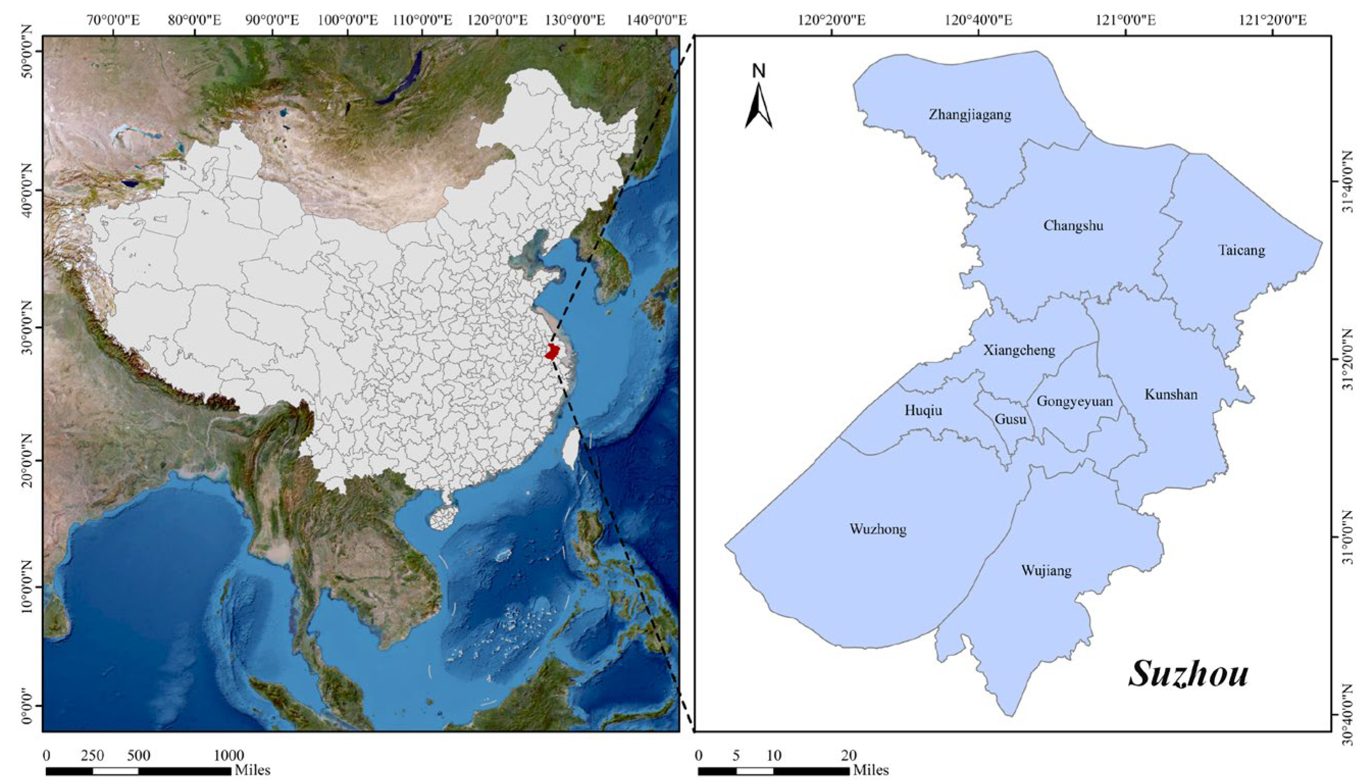
2.1. Overview of the Study Area

Suzhou City is located in the Yangtze River Delta region, in Eastern China. It lies in the southeastern part of Jiangsu Province and benefits from a strategic geographic location with excellent transportation connections. The study area is situated within an economically developed region, characterised by a rich natural resource base and a diversified economic landscape. The city of Suzhou is undergoing a rapid process of urbanisation, accompanied by a high population density, particularly in the urban area and the surrounding industrial parks, where a considerable number of people are concentrated. As illustrated in Figure 1, at the conclusion of 2020, Suzhou encompassed five districts, namely Gusu District, Huqiu District (Hi-Tech District), Wuzhong District, Xiangcheng District, and Wujiang District, in addition to the Suzhou Industrial Park. Furthermore, four county-level cities were under the indirect administration of Zhangjiagang, Changshu, Taicang, and Kunshan. The city is comprised of 42 streets and 52 townships.

2.2. Data Sources

In consideration of the limitations of data availability, this study is based on the seventh population census data of Suzhou City. The focus is on the collection of POI data that reflect the characteristics of population distribution in Suzhou City, as well as data on nighttime lighting, land use, settlements, roads, GDP, and building footprints that indicate the intensity of human activities. For a comprehensive list of data sources, please refer to

Table 1. Basic data sources.

Data	Data Type	Resolution	Data Source
Population Data	Tables	/	District/County Level: The Seventh National Census Bulletin of Suzhou Street Level: China Population Census Data by Township, Town, and Street 2020
Administrative Boundary	Vector (Side)	/	Jiangsu Provincial Department of Natural Resources
POI	Vector (Point)	/	Goldmap
Land use	Raster	30 m	China Multi-period Land Use/Cover Remote Sensing Monitoring Data (CNLUCC)
Night Lights	Raster	500 m	Resources and Environment Data Centre
Roads	Vectors (lines)	/	OSM datasets
Settlements	Vector (Side)	/	Resources and Environment Data Centre
Building Footprint Data	Vector (Side)	/	3D-GloBFP
GDP	Raster	1 km	Resources and Environment Data Centre

.

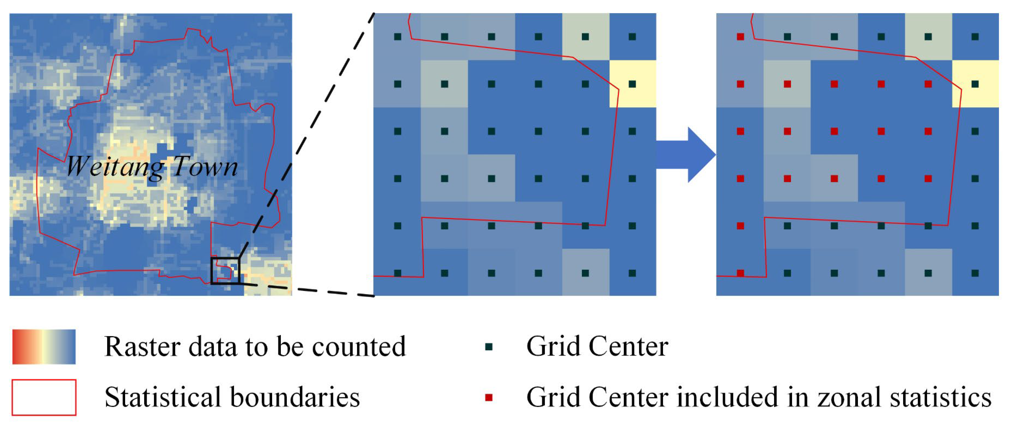
2.3. Data Processing

Given the inconsistency of the adopted data in terms of projection, resolution, and spatial extent, it is necessary to pre-process the original data before proceeding with the production of the dataset. This study ensures data consistency by applying various interpolation methods and high-precision coordinate transformations, minimizing the negative impact of conversion on model accuracy. Based on a literature-supported analysis [30,31], a 100 m resolution was selected for this study as it balances spatial accuracy and practical applicability, effectively capturing population clustering and spatial relationships, and aligns with international datasets like WorldPop to facilitate comparison and validation. All data were resampled to this resolution, with appropriate interpolation methods used to minimize spatial information loss: nearest-neighbour interpolation was applied to land use data to prevent mixed, unrealistic categories, while bicubic interpolation was used for GDP and nighttime light data to preserve detail and ensure smooth transitions. Additionally, the projection coordinates were uniformly converted to the Albers equal-area projection, suitable for the Chinese region, to reduce geometric distortion and coordinate shifts, thereby improving model accuracy.

3. Methodology

The objective of this study is to construct an optimised population spatialisation model by combining the Human Footprint Index (HFI) and the hierarchical feature coding method. This approach is intended to enhance the accuracy of population prediction in areas with different population densities. In particular, the study initially collates pertinent demographic and spatial data for Suzhou City. Following this, a kernel density analysis of the POI data is conducted, after which a hierarchical feature coding method is employed to process the input POI features. This is performed in order to more effectively capture the complexity of the population distribution within different regions. The initial predicted population spatial distribution weights were obtained through the application of a random forest model. To address the issue of data smoothing that is often associated with random forest, the study considers the characteristics of human activities within the study area and constructs HFI to correct these data, thereby reflecting the impact of human activities on population distribution. The final step is to evaluate the efficacy of the proposed model in enhancing prediction accuracy. This is achieved by comparing it with the traditional random forest model and the international public dataset (WorldPop). The technology roadmap is illustrated in Figure 2.

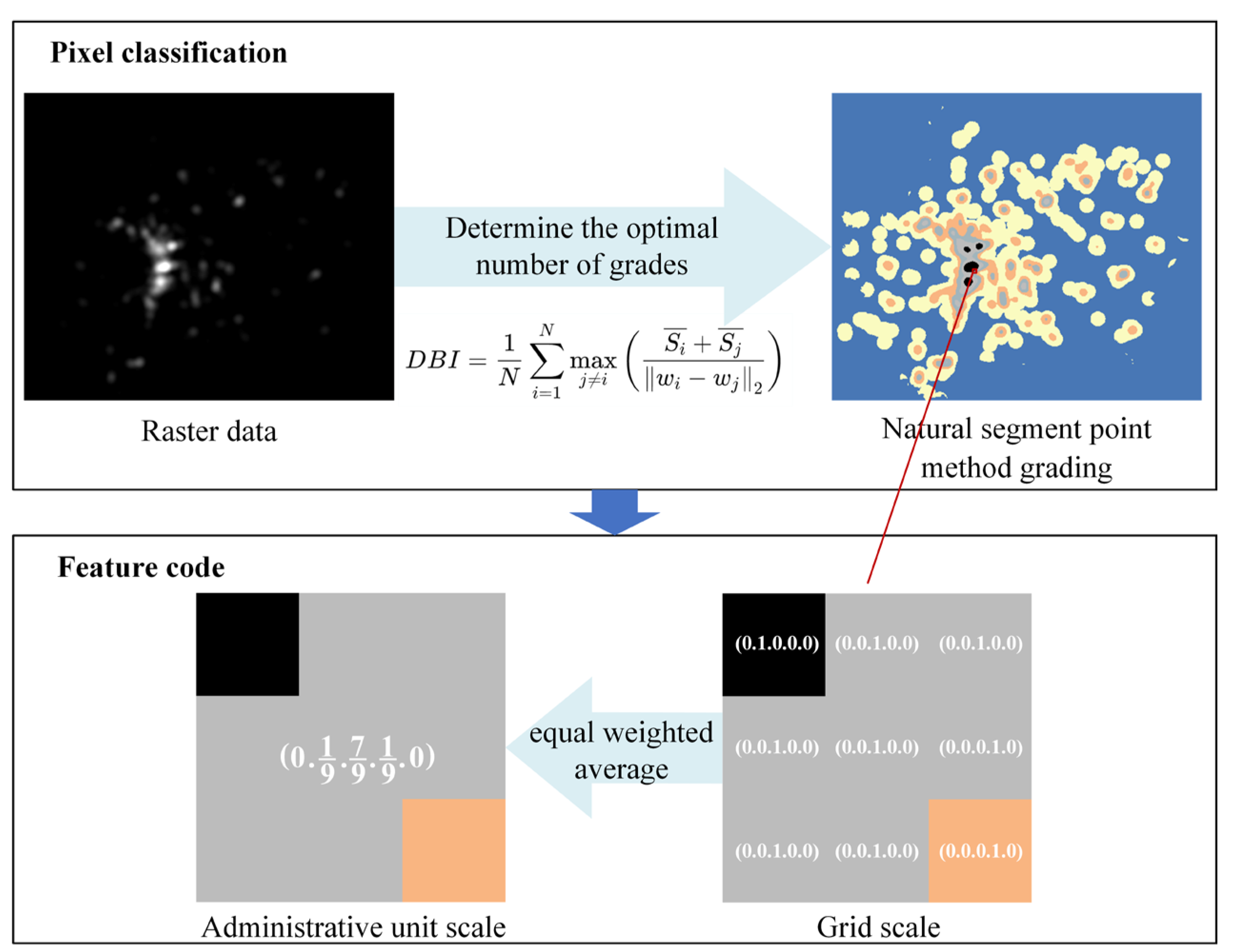
3.1. Hierarchical Feature Coding

In the context of population spatialisation, direct data assignment is often associated with significant errors, particularly at larger spans of scales (e.g., from administrative units to grid cells). The majority of traditional random forest-based population spatialisation studies input features directly into the model, which often results in the simplification of data and the loss of pertinent information. To address this issue, this study proposes an innovative hierarchical feature coding method to effectively handle complex spatial data.

The fundamental principle of hierarchical feature coding is the establishment of consistent classification criteria for raster data at varying scales, thereby facilitating the integration and unified analysis of multi-scale information. The process of hierarchical feature coding enables the capture of the multi-level structure of the data in greater detail by dividing the original features into multiple classes. The natural breaks method can divide intervals based on the internal characteristics of the data, effectively highlighting regions of natural clustering for high or low-frequency values, thus more accurately representing the distribution characteristics of different data. In particular, this study initially employs the natural breakpoint method to categorise feature values into k + 1 levels. This entails transforming continuous data into discrete and comparable levels through hierarchical processing. Subsequently, the optimal number of levels is determined using the Davies-Bouldin index (DBI). This process ensures variability and representativeness among the grades, thus enhancing the expressiveness of the features. The DBI is calculated in accordance with the following equation:

$$DBI={\displaystyle \frac{1}{N}}\sum _{i=1}^N{max}_{j\ne i}\left({\displaystyle \frac{\overline{S_i}+\overline{S_j}}{{∥w_i-w_j∥}_2}}\right)$$

(1)

where N is the total number of clusters, i, j are the cluster numbers, $S_i$, $S_j$ are the dispersion within clusters i and j, respectively, and $w_i$, $w_j$ are the centre of mass of the ith and jth cluster, respectively.

In accordance with the aforementioned methodology, the features are encoded in accordance with the established hierarchical classification, the resulting hierarchical results are represented in the form of feature vectors, which are then made available to the machine learning model, and finally, these feature vectors are employed as inputs to the random forest model. In summary, if the grid value is associated with the kth rank, the feature value is assigned a value of 1 at the kth rank encoding of the corresponding feature vector and a value of 0 at the other rank encodings. For example, the natural breakpoint method classifies the feature data into four ranks, plus one additional rank, resulting in a total of five ranks. The five ranks are as follows: 0, (0, 0.45), [0.45, 2.27), [2.27, 13.47), and [13.47, 455.46]. The grid with a value of 16.25 is designated as grid I. The corresponding feature vector of grid I is encoded as (0, 0, 0, 0, 1). A schematic diagram of the hierarchical feature coding method is provided in Figure 3 for reference.

3.2. Random Forest

The random forest (RF) algorithm is a commonly used machine learning method for classification and regression tasks, classified as an ensemble learning technique. Its core principle is to improve model performance by creating numerous decision trees and combining their predictions. The random forest algorithm comprises several key steps. (1) Bootstrap sampling: During the training process, random forest randomly draws multiple subsets from the training data by means of bootstrap sampling (i.e., sampling with replacement), and each subset is utilised to train an individual decision tree. This implies that the training data for each tree are not identical. (2) Random selection of features: in the process of splitting each decision tree, rather than utilising all the features to identify the optimal splitting point, a subset of features is randomly selected from the full set for the purpose of splitting. This has the effect of reducing the correlation between features and thus improving the model’s ability to generalise. (3) Integrated decision-making: in classification tasks, random forest determines the final category through a majority voting process; in regression tasks, the prediction is calculated as the mean.

The primary parameters associated with random forests include the following:

(1)

n_estimators: This parameter defines the number of trees in the forest. Increasing the number of trees improves model stability and accuracy, but also increases computation time. A balance must be struck between performance and efficiency.

(2)

max_depth: This controls the maximum depth of each tree, preventing excessive growth and overfitting. Deeper trees capture more details but may lead to overfitting, while shallower trees may underfit the data.

(3)

max_features: This determines how many features to consider for each split. A lower value reduces feature correlation between trees, improving diversity and reducing overfitting, but may also decrease model accuracy if set too low.

(4)

min_samples_split: This sets the minimum number of samples required to split a node. A higher value results in simpler trees by preventing splits in nodes with few samples, thus reducing overfitting, but might also make the model too simplistic.

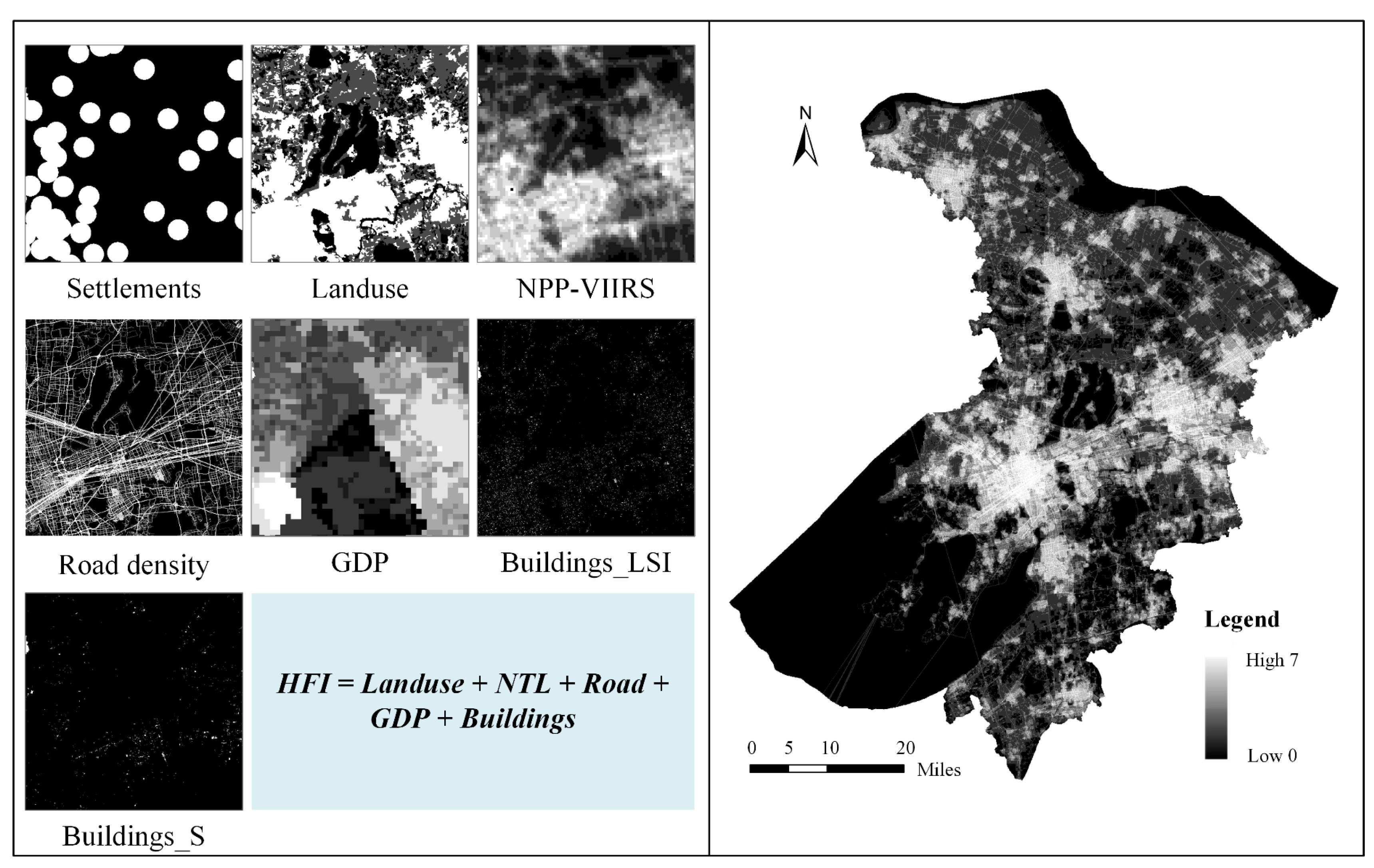
3.3. Human Footprint Index

The Human Footprint Index is a quantitative index for evaluating the intensity of human activities. The construction factors of this index are often optimised according to different research purposes and the characteristics of the study area in question [32]. In this study, seven factors were chosen based on existing research and the characteristics of human activities in the study area, focusing on how the intensity of human activity influences the spatial distribution of the population in Suzhou. These factors were selected from five aspects, namely land use, power facilities, traffic accessibility, socio-economic level, and building environment. The seven factors are settlement, land use, night lighting, road density, GDP, building area, and building shape index. The Human Footprint Index of Suzhou was constructed at a 100 m resolution. The raster of each data type was reassigned points on a 0–10 scale according to the different evaluation methods. The Human Footprint Index (HFI) was constructed by weighting the seven factors after resampling and reclassification to reflect the intensity of human activities. This was then used to correct the weights of the spatialisation of the population. The HFI is calculated using the following formula:

$$HFI=Landuse+NTL+Road+GDP+Buildings$$

(2)

where HFI denotes Human Footprint Index, Landuse denotes Land Use Intensity, NTL denotes Night Time Lighting Intensity, Road denotes Road Impact, GDP denotes Socio-Economic Level, and Buildings denotes Built Environment.

3.4. Weighting Corrections and Population Distribution

3.4.1. Weight Correction

The indiscriminate assignment of weights to each empty pixel by random forest, coupled with its reduced sensitivity to spatial heterogeneity, gives rise to significant errors in the prediction results. In order to accurately identify areas with no human distribution and simultaneously correct the population distribution weights of other locations, this study employs HFI data to rectify the predicted weight layer in accordance with the premise that the intensity of human activities is positively correlated with the population distribution. This entails adjusting the weights of locations where the HFI is 0 and applying the formula to modify the weights of other locations. The correction formula is as follows:

$$w_{pixel\text{\_}j}*=w_{pixel\_j}\times {\left({\displaystyle \frac{{HFI}_{pixel\_j}}{{HFI}_{max}}}\right)}^{\theta }\times \gamma$$

(3)

where $w_{pixel\_j}*$ is the weight after correction, $w_{pixel\_j}$ is the weight before correction, ${HFI}_{pixel\_j}$ is the HFI value of grid j, ${HFI}_{max}$ is the largest HFI value of all the corrected grids, and $\theta$ is the tuning parameter, which controls the effect of HFI on the result of the correction; $\gamma$ represents the coefficient that adjusts and constrains the range of correction weights.

3.4.2. Population Decomposition

In this study, the census data were decomposed from the district and county scale to the grid scale using the corrected weights with the following formula:

$${POP}_{pixel\_j}={POP}_{district\_i}\times {\displaystyle \frac{w_{pixel\_j}}{w_{district\_i}}}$$

(4)

where ${POP}_{pixel\_j}$ represents the projected population of grid j, ${POP}_{district\_i}$ represents the census population of district I, $w_{pixel\_j}$ refers to the population weight of grid j, and $w_{district\_i}$ represents the sum of the population weights of all the grids in district i to which grid j belongs.

3.5. Validation of Accuracy

In the absence of a definitive pixel-level population dataset, the total predicted population is validated by comparing it with the census data for each street. The study first uses zonal statistical tools to aggregate the gridded population data into vector boundaries at the street level, as illustrated in Figure 4.

Based on this foundation, the accuracy of the predicted dataset is validated using the following indicators: mean absolute error (MAE), which shows the average difference between predicted and actual values; root mean square error (RMSE), which quantifies prediction errors; coefficient of determination (R²), indicating how well the model explains data variation; mean relative error (MRE), which captures the relative difference between predictions and actual values [16,33]; and Pearson correlation coefficient, which measures the strength and direction of the relationship between predictions and actual values [34]. The calculation formulas for each indicator are as follows:

$$MAE={\displaystyle \frac{1}{n}}\sum _{i=1}^n\left|Predic{t}_i-Rea{l}_i\right|$$

(5)

$$RMSE=\sqrt{{\displaystyle \frac{1}{n}}\sum _{i=1}^n{\left(Predic{t}_i-Rea{l}_i\right)}^2}$$

(6)

$$R^2=1-{\displaystyle \frac{\sum _i{\left(Rea{l}_i-Predic{t}_i\right)}^2}{\sum _i{\left(Rea{l}_i-\overline{Real}\right)}^2}}$$

(7)

$$MRE={\displaystyle \frac{1}{n}}\sum _{i=1}^n\left|{\displaystyle \frac{Predic{t}_i-Rea{l}_i}{Rea{l}_i}}\right|$$

(8)

$$Pearson={\displaystyle \frac{\sum ({Predict}_i-\overline{Predict})({Real}_i-\overline{Real})}{\sqrt{\sum ({Predict}_i-\overline{Predict}{)}^2\sum ({Real}_i-\overline{Real}{)}^2}}}$$

(9)

where $Predic{t}_i$ represents the predicted population of street i, $Rea{l}_i$ represents the census count of street i, $\overline{Real}$ is the mean population across all streets, and n denotes the total number of streets.

4. Experiments and Results

4.1. Random Forest-Based Weight Prediction

A Point of Interest (POI) represents location and attribute information about various facilities within a city. The distribution density and agglomeration trends of POIs can effectively indicate population aggregation patterns. POI data offer several advantages, including easy access, detailed current information, large volumes, and high positioning accuracy, which help overcome traditional data limitations such as low spatial accuracy and long updating periods [2]. This makes POI data essential for population spatialisation. After data cleaning, this study extracted 13 types of POI data related to population distribution using kernel density analysis. The POI types and their rationale are presented in

Table 2. POI types and reasons for selection.

Category	POI Type	Reason for Selection
Daily Life	Dining	Reflects basic living needs and daily activities, effectively representing population aggregation and activity frequency.
	Shopping
	Accommodation Services
	Life Services
Business	Business and Residential Areas	Primary venues for economic activity in densely populated areas, influencing population distribution and movement.
	Financial and Insurance
Transportation and Public Facilities	Transportation Facilities	Provides regional accessibility and convenience, directly affecting population spatial distribution and activity patterns.
	Public Facilities
Education and Culture	Science, Education, and Cultural Facilities	Concentrated in population-dense areas, reflecting the distribution of social and cultural activities.
Health and Medical Care	Medical Care	Core to residents’ daily health needs, often located in densely populated areas, directly impacting population spatialisation.
Recreation and Tourism	Sports and Leisure	Attracts large numbers of residents and tourists, reflecting spatial distribution in leisure and tourism activities.
	Scenic Spots
Government and Social Organisations	Government Agencies and Social Organisations	Centres of regional social and administrative activities, directly influencing social structure and population density.

. A hierarchical feature coding method was then used to obtain POI feature vectors at both grid and administrative unit scales.

For the analysis, the 13 types of POI features from 10 districts in Suzhou City were used as training samples in the random forest model, with the features divided into training and testing sets. Considering model accuracy, generalisation capability, and computational efficiency, the random forest parameters were set as follows: n_estimators was set to 100 to balance stability and computational cost; max_depth was set to None to allow the model to capture complex data patterns, with experiments confirming no overfitting risk; max_features was left at the default to ensure random feature selection during splits, enhancing model robustness; and min_samples_split also used the default to prevent overly small sample nodes, improving model performance. These parameter settings ensured a balance between model accuracy and efficiency, strengthening prediction stability and generalisation. Using administrative boundary data from Suzhou, a 100 m × 100 m grid was established, and feature statistics were calculated based on this grid. The trained random forest model was then applied to predict population weights for each grid cell.

4.2. Construction of the Human Footprint Index

As a significant indicator of the impact of human activities on the environment, the Human Footprint Index is a key element in the analysis of population distribution. In consideration of the characteristics of the study area and the manner of human activities, this study has selected the following seven factors for the construction of the Human Footprint Index. In accordance with the methodologies employed in existing studies on diverse factors [35], the present study initially reclassified the seven types of factors following resampling. In accordance with the various methodologies employed, the factors were assigned a score on a scale of 0–10, with a higher score denoting a greater intensity of impact resulting from human activities.

(1)

Land use

Land use is an important factor that reflects the level of human activity. Although some scholars posit that all populations are situated within built-up areas, this study, in examining land use data, suggests that there may be instances where this is not the case. In particular, this study assigns scores based on land types: 10 points for building land, 3 for agricultural land, 2 for grazing land, 1 for forestry, and 0 for all other categories.

(2)

Settlements

Settlements where people live and work indicate human activity intensity and thus population distribution. In accordance with Sanderson et al.‘s methodology for assigning values to settlements, the study assigns a score of 8 within the boundaries of settlements [24,36] and a score of 0 for other areas.

(3)

Night lights

Nighttime lighting reflects population distribution at night and captures human activity changes, especially in rapidly urbanising areas. DN values in the nighttime lighting data are processed, assigning 0 to rasters with DN values of 0 and scores from 1 to 10 to those with DN values greater than 0, based on deciles.

(4)

Roads

The relationship between roads and population distribution is close, as road accessibility often promotes population clustering and movement. When considering road impacts, existing studies typically create buffers and assign subjective values based on road grade and distance from the centreline [37,38]. This subjectivity can introduce inconsistencies, potentially leading to inaccurate representations of road influence on population distribution. To address this, this study uses road density to evaluate the impact of road classifications on population distribution patterns, while also considering road grade. Referring to related studies and the road classifications in Gaode Maps, OSM road data were refined and reclassified, with different weights assigned according to road type (see

Table 3. OSM road classification method and weight assignment.

Road Type	OSM Classification	Weight
Elevated and Express Roads	motorway, motorway_link, trunk, trunk_link	1.0
Main Roads	primary, primary_link, secondary, secondary_link	0.8
Secondary Roads	tertiary, tertiary_link	0.6
Branch Roads	residential, unclassified	0.4
Internal Roads and Others	footway, pedestrian, cycleway, steps, bridleway, path, track, living_street, service	0.2

for specific classifications and values). The weighted road density was then converted to raster data, processed similarly to nighttime light data. This weighted approach, combining road density with road grade, more comprehensively accounts for road functionality and importance, supporting a more objective construction of the Human Footprint Index.

(5)

GDP

GDP reflects a region’s economic activities and is closely related to land use, resource consumption, and population distribution. Including GDP in the Human Footprint Index (HFI) provides insights into the impact of economic development on environmental pressure and population distribution. The assignment method is similar to that used for nighttime lights data.

(6)

Building area

The floor space of a given area can be used as a proxy for the degree of urbanisation and the space occupation of human activities. It can, therefore, be employed as an effective indicator of the development and use of land by human beings, and thus of the spatial distribution pattern of the population. The method of assignment is also that of nighttime lights data.

(7)

Building Shape Index

The Building Shape Index is used to evaluate the complexity of building forms and their spatial efficiency, calculated as the ratio of a building’s perimeter to its area. Integrating this index into the Human Footprint Index provides a clearer picture of natural resource consumption and the ecological impact of human activities, as it reflects building layout and density. The assignment method mirrors that used for nighttime lights data.

Based on the above methodology, the 100 m Human Footprint Index dataset of Suzhou City was constructed as shown in Figure 5.

4.3. Spatialisation of Population Data Based on HFI Correction

Given the low sensitivity of random forests to spatial heterogeneity, which may result in the smoothing of the data, this study considered the impact of human activities on population distribution in the study area. To this end, Equation (3) was employed to correct the weighting layer predicted by random forests. In particular, the study assigns the grid with no human activities a value of zero and makes several attempts to determine the optimal weight adjustment parameter, represented by a value of 1.5, and the proportionality constant, represented by a value of 1. This method entails the redistribution of the population from the administrative unit scale to the grid scale, thereby facilitating the spatialisation of the population in Suzhou City based on the correction of HFI (HFIPop).

To further test the accuracy of the proposed method, this study conducted a population spatialisation experiment based on the traditional random forest method (RFPop) as well as a population spatialisation experiment based on the HFI correction without hierarchical feature coding method (NoHFEPop). The results were then subjected to analysis in comparison with the international public dataset WorldPop. The final population spatialisation results for Suzhou are presented in Figure 6.

The graphical analysis reveals that the population of Suzhou City is concentrated in the city centre, forming four distinct high-density nuclei: Gusu District, Yangshe Town (Zhangjiagang City), Qinchuan Street (Changshu City), and Yushan Town (Kunshan City). While the spatial patterns of the three datasets are similar, notable differences exist. The population dataset based on the traditional random forest model (RFPop) exhibits low spatial heterogeneity and excessive smoothness, hindering its ability to distinguish high-density areas and inter-regional differences. In contrast, the WorldPop dataset, though it shows some overall spatial characteristics, is relatively homogeneous and fails to reflect actual human activities and population aggregation, missing subtle distinctions between urban and suburban regions.

HFIPop, by incorporating human activity intensity corrections, effectively captures the spatial heterogeneity of population distribution, addressing the RF model’s shortcomings. For example, it accurately identifies population distribution in peripheral suburbs like Bixi Street and Taoyuan Town, delineating high-density kernels in Gusu District and Yangshe Town, while RFPop fails to capture these nuances. The smoothing nature of RFPop reduces spatial heterogeneity, impairing its reflection of actual distribution characteristics. Although WorldPop provides a broad spatial perspective, its homogeneity limits its effectiveness in portraying the impact of human activities. In comparison, HFIPop enhances the ability to discern contrasts between urban and suburban areas and illustrates the influence of human activities on population aggregation patterns. In summary, HFIPop offers superior spatial resolution and more precise population projections than RFPop and WorldPop.

4.4. Accuracy Validation and Result Analysis

4.4.1. Accuracy Comparison Validation

The accuracy of the HFIPop, RFPop, NoHFEPop, and WorldPop datasets is validated using the following equations: (5)–(9), respectively. The results demonstrate that the HFIPop dataset exhibits a high level of prediction accuracy, with an R² value of 0.928 and a MAPE of 16.75%. The specific results are presented in

Table 4. Comparison results of the accuracy of each type of dataset.

	HFIPop	RFPop	NoHFEPop	WorldPop
MAE	17,587.54220	29,121.32409	22,989.21765	38,288.72771
RMSE	27,446.31164	42,138.12982	36,129.38270	56,855.34566
R2	0.92839	0.81681	0.87829	0.692692533
MAPE	16.75170	25.32145%	21.46892%	29.20127102%
Pearson	0.96364	0.90820	0.936877	0.93634

.

Based on the results presented in Table 4, the HFIPop model demonstrates a marked improvement in performance across several key metrics compared to RFPop, NoHFEPop, and WorldPop. Specifically, HFIPop exhibits a significantly lower Mean Absolute Error (MAE) of 17,587.54 and Root Mean Square Error (RMSE) of 27,446.31, relative to the higher error values observed for RFPop (MAE: 29,121.32, RMSE: 42,138.13), NoHFEPop (MAE: 22,989.22, RMSE: 36,129.38), and WorldPop (MAE: 38,288.73, RMSE: 56,855.35). These results suggest that HFIPop is more precise in spatialising population data, capturing fine-grained variations with reduced prediction errors. Moreover, the R² value for HFIPop (0.9284) is notably higher than that of RFPop (0.8168), NoHFEPop (0.8783), and WorldPop (0.6927), indicating a stronger capacity for explaining the variance in the population distribution. Furthermore, the MAPE for HFIPop (16.75%) outperforms that of RFPop (25.32%), NoHFEPop (21.47%), and WorldPop (29.20%), suggesting that HFIPop not only achieves higher accuracy but also offers a more stable performance across different population density zones.

In addition to these error metrics, the Pearson correlation coefficients further underscore the robustness of the HFIPop model in capturing the underlying spatial patterns of the population distribution. The Pearson correlation for HFIPop (0.9636) is substantially higher than those for RFPop (0.9082), NoHFEPop (0.9369), and WorldPop (0.9363), which indicates a stronger linear relationship with the actual population data. This enhanced correlation reflects HFIPop’s superior capacity to align with the real-world distribution of the population, validating its effectiveness in population spatialisation. Collectively, these findings highlight the substantial improvements in prediction accuracy, error reduction, and spatial pattern alignment that HFIPop achieves by integrating HFI correction and hierarchical feature coding, positioning it as a more reliable and scientifically rigorous tool for population spatialisation in complex geographical contexts.

4.4.2. Validation of Partitioning Accuracy

In order to explore the applicability of the method proposed in this study in different population density regions, the K-Means clustering method is employed to divide the streets of Suzhou City into three types of population density zones: high, medium, and low. Furthermore, the differences in the performance of the HFIPop, RFPop, and WorldPop datasets in these zones are validated. The results are presented in Figure 7, which demonstrates that there are notable discrepancies in the performance of each model across different population density regions.

In the low- and medium-density regions, the HFIPop model demonstrates superior performance across several key metrics. Notably, the MAE and RMSE values of HFIPop in both regions (low: 11,782.29 and 17,036.44; medium: 21,946.35 and 33,278.59) are substantially lower than those of RFPop and WorldPop, indicating a more accurate prediction of population distribution. The MAPE for HFIPop in both low- (19.46%) and medium- (15.53%) density regions is also markedly lower than that of RFPop and WorldPop, reflecting better consistency in percentage error. Moreover, the R² values of HFIPop in these regions (low: 0.83; medium: 0.92) are higher than those of the competing models, demonstrating HFIPop’s superior ability to explain the variance in population distribution. The Pearson correlation coefficients of HFIPop in the low- and medium-density regions (0.93 and 0.96, respectively) further support this, indicating a stronger linear relationship with the actual population data compared to RFPop and WorldPop. In contrast, in the high-density region, while the MAE and RMSE of HFIPop (14,632.35 and 21,156.01) remain lower than those of WorldPop (65,991.97 and 74,109.70), they are slightly higher than RFPop’s values (14,268.37 and 23,286.11), indicating a more balanced performance. Despite this, HFIPop’s MAPE (9.33%) remains lower than WorldPop’s (48.54%), emphasizing its superior accuracy in high-density areas. The R² value of HFIPop in the high-density region (0.78) is significantly higher than that of WorldPop (−1.72), suggesting that HFIPop is more reliable in explaining population distribution in this region. Furthermore, the Pearson coefficient of HFIPop in the high-density region (0.99) is notably higher than both RFPop (0.98) and WorldPop (0.90), reinforcing the conclusion that HFIPop better captures the spatial distribution in high-density areas.

In summary, the method based on HFI correction and combined with hierarchical feature coding demonstrates enhanced stability and accuracy in low-, medium-, and high-density regions, particularly in low- and medium-density regions, thereby markedly enhancing the capacity to adapt to complex population distribution. This indicates that the HFI correction model has considerable potential for application in diverse population density regions and represents a more comprehensive and accurate model for population spatialisation optimisation.

5. Discussion and Conclusions

5.1. Adaptability of the Model to Different Regions

In low- and medium-density areas, models based on the Human Footprint Index (HFI) correction demonstrate strong performance due to their ability to effectively handle spatial heterogeneity. These regions are characterised by relatively dispersed human activity, posing a challenge for traditional random forest models that struggle to capture such complexity. By adjusting for variations in human activity intensity, the HFI correction model excels at identifying subtle aggregation effects, such as infrastructure, land use, and accessibility. These often overlooked but crucial features are key to accurately predicting population distribution in these areas. The model’s ability to account for these nuances and adapt flexibly to the varying population patterns in low-density regions significantly reduces prediction errors, yielding lower MAE and RMSE values compared to RFPop and WorldPop. The high R² and Pearson correlation further emphasize the model’s effectiveness in explaining population distribution disparities.

Conversely, in high-density regions, the relatively uniform geographical and functional characteristics result in persistently high population densities, and human activity becomes more complex and concentrated, leading to a saturation effect. In such areas, the performance gains of the HFI correction model diminish. Extreme population density, coupled with rapid urbanisation, complicates the model’s ability to capture the dynamic and diverse nature of human activity. While HFI correction can improve model performance across all density levels, its true potential is best realised in areas where human activity is more heterogeneous and less saturated. These findings suggest that while the HFI correction model can enhance performance in both low and medium-density areas, further refinement may be required to address the complexities of high-density regions, particularly through the integration of more dynamic and localised features that better capture the nuances of urbanised spaces.

5.2. Limitations and Future Outlook

Despite the demonstrated improvements, the HFI-modified population spatialisation optimisation model does have certain limitations, particularly in high-density and highly urbanised areas. As previously discussed, extreme population densities and the saturation of human activities in these regions pose significant challenges to the model’s ability to capture subtle variations in population distribution. Rapid urbanisation further complicates the model’s predictive accuracy, as population activity patterns are highly dynamic and not always fully represented by static indicators like the Human Footprint Index (HFI). This underscores the need for further refinement, specifically to improve the model’s adaptability to the complex dynamics of urbanised environments, where human activities are constantly shifting. Additionally, the model’s performance is heavily dependent on data quality and availability. In regions with sparse or low-quality data, the model’s ability to generate accurate population predictions may be constrained. It is crucial to explore more stable and high-quality data sources and to deeply mine the information they provide.

Looking ahead, future research should focus on addressing these challenges by integrating more detailed, adaptable, and dynamic human activity indicators. This may involve incorporating more detailed functional zoning data, real-time mobility data (such as Baidu Huiyan data, mobile signal data, etc.) to better capture the evolving population dynamics in different spatial contexts. For urban areas, it may be beneficial to introduce targeted urban intensity indices as new correction factors, further enhancing the model’s ability to represent rapid changes in urban environments and spatial heterogeneity. For regions outside of China, due to differences in socio-economic factors and urbanisation patterns, data adaptation based on local land use types, economic activity densities, and other factors may be required. Additionally, improving the model’s parameter adaptability, considering resolution optimisation for specific sub-regions, or utilizing more computationally powerful models (e.g., CNNs) will help optimize its performance in diverse environments, making it a more reliable tool for urban planning, resource allocation, and policy-making. Another important direction for future work is to establish regional data-sharing mechanisms, which will facilitate the widespread application of this model in different geographic areas. Strengthening user training and developing more intuitive user interfaces will also be crucial for promoting the model’s practical application in urban management and planning. Ultimately, integrating socio-economic factors, environmental data, and more dynamic urban indicators will be key to refining the model and improving its accuracy, providing a more comprehensive and adaptable tool for urban management in various contexts.

5.3. Conclusions

The population spatialisation optimisation model proposed in this study, based on the Human Footprint Index (HFI) correction and combined with hierarchical feature coding, demonstrates notable advantages in different population density regions. The study’s findings can be summarised as follows:

(1)

The coefficient of determination (R²) for the HFI-corrected population spatialisation dataset of Suzhou City is 92.8%, reflected an improvement of 11 percentage points over the random forest model alone and 23 percentage points compared to the WorldPop dataset. The Pearson correlation coefficient of 0.96 further confirms its strong alignment with actual population data.

(2)

The HFI-corrected optimisation model is particularly effective in medium-density areas, achieving an accuracy of 92.3% and a Pearson correlation of 0.96. This suggests the model effectively captures the complex relationship between human activities and population distribution, particularly in dispersed regions.

(3)

The hierarchical feature coding methodology significantly reduces inaccuracies in population spatialisation across different scales, increasing the model’s precision by an additional five percentage points and enhancing its overall applicability and reliability.

References

1. Dmowska, A.; Stepinski, T.F. A High Resolution Population Grid for the Conterminous United States: The 2010 Edition. Comput. Environ. Urban Syst. 2017, 61, 13–23. [Google Scholar] [CrossRef]
2. Zhao, S.; Liu, Y.; Zhang, R.; Fu, B. China’s Population Spatialization Based on Three Machine Learning Models. J. Clean. Prod. 2020, 256, 120644. [Google Scholar] [CrossRef]
3. Mei, Y.; Gui, Z.; Wu, J.; Peng, D.; Li, R.; Wu, H.; Wei, Z. Population Spatialization with Pixel-Level Attribute Grading by Considering Scale Mismatch Issue in Regression Modeling. Geo-Spat. Inf. Sci. 2022, 25, 365–382. [Google Scholar] [CrossRef]
4. Bao, W.; Gong, A.; Zhao, Y.; Chen, S.; Ba, W.; He, Y. High-Precision Population Spatialization in Metropolises Based on Ensemble Learning: A Case Study of Beijing, China. Remote Sens. 2022, 14, 3654. [Google Scholar] [CrossRef]
5. He, M.; Xu, Y.; Li, N. Population Spatialization in Beijing City Based on Machine Learning and Multisource Remote Sensing Data. Remote Sens. 2020, 12, 1910. [Google Scholar] [CrossRef]
6. Zhao, M.; Cheng, W.; Zhou, C.; Li, M.; Wang, N.; Liu, Q. GDP Spatialization and Economic Differences in South China Based on NPP-VIIRS Nighttime Light Imagery. Remote Sens. 2017, 9, 673. [Google Scholar] [CrossRef]
7. Dong, C.; Zhang, Y.; Kang, F. Renkou Kongjianhua Jishu; China Population Publishing House: Beijing, China, 2024; ISBN 978-7-5101-8908-1. [Google Scholar]
8. Leyk, S.; Gaughan, A.E.; Adamo, S.B.; De Sherbinin, A.; Balk, D.; Freire, S.; Rose, A.; Stevens, F.R.; Blankespoor, B.; Frye, C.; et al. The Spatial Allocation of Population: A Review of Large-Scale Gridded Population Data Products and Their Fitness for Use. Earth Syst. Sci. Data 2019, 11, 1385–1409. [Google Scholar] [CrossRef]
9. Zhao, Y.; Li, Q.; Zhang, Y.; Du, X. Improving the Accuracy of Fine-Grained Population Mapping Using Population-Sensitive POIs. Remote Sens. 2019, 11, 2502. [Google Scholar] [CrossRef]
10. Stevens, F.R.; Gaughan, A.E.; Linard, C.; Tatem, A.J. Disaggregating Census Data for Population Mapping Using Random Forests with Remotely-Sensed and Ancillary Data. PLoS ONE 2015, 10, e0107042. [Google Scholar] [CrossRef]
11. Ye, T.; Zhao, N.; Yang, X.; Ouyang, Z.; Liu, X.; Chen, Q.; Hu, K.; Yue, W.; Qi, J.; Li, Z.; et al. Improved Population Mapping for China Using Remotely Sensed and Points-of-Interest Data within a Random Forests Model. Sci. Total Environ. 2019, 658, 936–946. [Google Scholar] [CrossRef]
12. Xu, X. China Population Spatial Distribution Kilometer Grid Dataset. Data Registration and Publishing System of Resource and Environmental Science Data Center of Chinese Academy of Sciences. 2017. Available online: http://www.resdc.cn/DOI/DOI.aspx?DOIid=32 (accessed on 2 March 2024).
13. Chen, Y.; Xu, C.; Ge, Y.; Zhang, X.; Zhou, Y. A 100 m Gridded Population Dataset of China’s Seventh Census Using Ensemble Learning and Big Geospatial Data. Earth Syst. Sci. Data 2024, 16, 3705–3718. [Google Scholar] [CrossRef]
14. Goodchild, M.F.; Lam, N.S. Areal Interpolation: A Variant of the Traditional Spatial Program. Geo-Process. 1980, 1, 297–312. [Google Scholar]
15. Tobler, W.R. Smooth Pycnophylactic Interpolation for Geographical Regions. J. Am. Stat. Assoc. 1979, 74, 519–530. [Google Scholar] [CrossRef]
16. Guo, W.; Zhang, J.; Zhao, X.; Li, Y.; Liu, J.; Sun, W.; Fan, D. Combining Luojia1-01 Nighttime Light and Points-of-Interest Data for Fine Mapping of Population Spatialization Based on the Zonal Classification Method. IEEE J. Sel. Top. Appl. Earth Obs. Remote Sens. 2023, 16, 1589–1600. [Google Scholar] [CrossRef]
17. Zhang, Y.; Wang, H.; Luo, K.; Wu, C.; Li, S. Study on Spatialization and Spatial Pattern of Population Based on Multi-Source Data—A Case Study of the Urban Agglomeration on the North Slope of Tianshan Mountain in Xinjiang, China. Sustainability 2024, 16, 4106. [Google Scholar] [CrossRef]
18. Liu, L.; Cheng, G.; Yang, J.; Cheng, Y. Population Spatialization in Zhengzhou City Based on Multi-Source Data and Random Forest Model. Front. Earth Sci. 2023, 11, 1092664. [Google Scholar] [CrossRef]
19. Wang, M.; Wang, Y.; Li, B.; Cai, Z.; Kang, M. A Population Spatialization Model at the Building Scale Using Random Forest. Remote Sens. 2022, 14, 1811. [Google Scholar] [CrossRef]
20. Wu, J.; Gui, Z.; Shen, li.; Wu, Y.; Liu, H.; Li, R.; Mei, Y.; Peng, D. Population Spatialization by Considering Pixel⁃Level Attribute Grading and Spatial Association. Geomat. Inf. Sci. Wuhan. Univ. 2022, 47, 1364–1375. [Google Scholar] [CrossRef]
21. Tan, M.; Liu, K.; Liu, L.; Zhu, Y.; Wang, D.; Min, T.; Kai, L.; Lin, L.; Yuanhui, Z.; Dashan, W. Spatialization of population in the Pearl River Delta in 30m grids using random forest model. Progress. Geogr. 2017, 36, 1304–1312. [Google Scholar] [CrossRef]
22. Guo, Y.; Li, X. Spatiotemporal changes of urban construction land structure and driving mechanism in the Yellow River Basin based on random forest model. Prog. Geogr. 2023, 42, 12–26. [Google Scholar] [CrossRef]
23. Qiu, G.; Bao, Y.; Yang, X.; Wang, C.; Ye, T.; Stein, A.; Jia, P. Local Population Mapping Using a Random Forest Model Based on Remote and Social Sensing Data: A Case Study in Zhengzhou, China. Remote Sens. 2020, 12, 1618. [Google Scholar] [CrossRef]
24. Sanderson, E.W.; Jaiteh, M.; Levy, M.A.; Redford, K.H.; Wannebo, A.V.; Woolmer, G. The Human Footprint and the Last of the Wild. BioScience 2002, 52, 891. [Google Scholar] [CrossRef]
25. Hua, T.; Zhao, W.; Cherubini, F.; Hu, X.; Pereira, P. Continuous Growth of Human Footprint Risks Compromising the Benefits of Protected Areas on the Qinghai-Tibet Plateau. Glob. Ecol. Conserv. 2022, 34, e02053. [Google Scholar] [CrossRef]
26. Tapia-Armijos, M.F.; Homeier, J.; Draper Munt, D. Spatio-Temporal Analysis of the Human Footprint in South Ecuador: Influence of Human Pressure on Ecosystems and Effectiveness of Protected Areas. Appl. Geogr. 2017, 78, 22–32. [Google Scholar] [CrossRef]
27. Woolmer, G.; Trombulak, S.C.; Ray, J.C.; Doran, P.J.; Anderson, M.G.; Baldwin, R.F.; Morgan, A.; Sanderson, E.W. Rescaling the Human Footprint: A Tool for Conservation Planning at an Ecoregional Scale. Landsc. Urban. Plan. 2008, 87, 42–53. [Google Scholar] [CrossRef]
28. González-Abraham, C.; Ezcurra, E.; Garcillán, P.P.; Ortega-Rubio, A.; Kolb, M.; Bezaury Creel, J.E. The Human Footprint in Mexico: Physical Geography and Historical Legacies. PLoS ONE 2015, 10, e0121203. [Google Scholar] [CrossRef]
29. Dong, C.; Qi, S.; Dai, Z.; Qiu, X.; Luo, T. Research on Accurate and Effective Identification of Ecosystem Surface Based on Human Footprint Index. Ecol. Indic. 2024, 162, 112013. [Google Scholar] [CrossRef]
30. Dong, N.; Yang, X.; Cai, H.; Huang, D. Suitability Evaluation of Gridded Population Distribution: Acase Study in Rural Area of Xuanzhou District, China. Acta Geogr. Sin. 2017, 72, 2310–2324. [Google Scholar] [CrossRef]
31. Luo, Y.; Dong, C.; Zhang, Y. Study on the Method of Evaluating the Suitable Grid for Population Spatialisation. J. Geo-Inf. Sci. 2023, 25, 896–908. [Google Scholar] [CrossRef]
32. Duan, Q.; Luo, L. Summary and Prospect of Spatialization Method of Human Activity Intensity: Taking the Qinghai-Tibet Plateau as an Ex- Ample. J. Glaciol. Geocryol. 2021, 43, 1582–1593. [Google Scholar] [CrossRef]
33. Chen, M.; Xian, Y.; Huang, Y.; Zhang, X.; Hu, M.; Guo, S.; Chen, L.; Liang, L. Fine-Scale Population Spatialization Data of China in 2018 Based on Real Location-Based Big Data. Sci. Data 2022, 9, 624. [Google Scholar] [CrossRef] [PubMed]
34. Wu, X.; Wang, H.; Zhao, A.; Xie, Y. Spatialization Research on Shanghai′s Population Based on Multi-Source Data and XGBoost Model. Geomat. Spat. Inf. Technol. 2024, 47, 33–36. [Google Scholar]
35. Duan, Q.; Luo, L. A Dataset of Human Footprint over the Qinghai-Tibet Plateau during 1990–2015. China Sci. Data 2020, 5, 303–312. [Google Scholar] [CrossRef]
36. Luo, L.; Duan, Q.; Wang, L.; Zhao, W.; Zhuang, Y. Increased Human Pressures on the Alpine Ecosystem along the Qinghai-Tibet Railway. Reg. Environ. Chang. 2020, 20, 33. [Google Scholar] [CrossRef]
37. Qu, Z.; Zhao, Y.; Luo, M.; Han, L.; Yang, S.; Zhang, L. The Effect of the Human Footprint and Climate Change on Landscape Ecological Risks: A Case Study of the Loess Plateau, China. Land 2022, 11, 217. [Google Scholar] [CrossRef]
38. Ayram, C.A.C.; Etter, A.; Díaz-Timoté, J.; Buriticá, S.R.; Ramírez, W.; Corzo, G. Spatiotemporal evaluation of the human footprint in Colombia: Four decades of anthropic impact in highly biodiverse ecosystems. Ecol. Indic. 2020, 117, 106630. [Google Scholar] [CrossRef]
Figure 1. Overview of the study area.
Ijgi 13 00429 g001
Figure 2. Technology roadmap.
Ijgi 13 00429 g002
Figure 3. Schematic diagram of hierarchical feature coding method.
Ijgi 13 00429 g003
Figure 4. Diagram of zonal statistical workflow.
Ijgi 13 00429 g004
Figure 5. Schematic diagram of the construction of the Human Footprint Index.
Ijgi 13 00429 g005
Figure 6. Spatialised dataset of population in Suzhou based on HFI correction (HFIPop). (A) is the spatialisation of the population dataset based on the Human Footprint Index correction (HFIPop), (B) is the spatialisation of population dataset based on traditional RF model projections (RFPop), and (C) is the WorldPop dataset).
Ijgi 13 00429 g006
Figure 7. Comparison of the accuracy of the precision partitions of each dataset. (a) Comparison of MAE for different models, (b) Comparison of RMSE for different models, (c) Comparison of R² for different models, (d) Comparison of MAPE for different models, (e) Comparison of Pearson for different models.
Ijgi 13 00429 g007aIjgi 13 00429 g007b