Pre-Dam Vltava River Valley—A Case Study of 3D Visualization of Large-Scale GIS Datasets in Unreal Engine

Abstract

This article explores the potential of the Unreal Engine as a tool for creating realistic 3D visualizations of large-scale areas (1000 km² and more) using GIS datasets. Unlike small-scale visualizations, large-scale visualizations are rare and often not public, which presents significant problems since they present different challenges and require different approaches. This article presents several relevant scientific studies and projects that have successfully used game engines for similar purposes. This case study focuses on the computational techniques used in Unreal Engine for the 3D visualization of GIS data and the potential application of Unreal Engine in large-scale geo-visualizations. It explores the potential for using GIS data within a game engine, including plug-ins that provide additional functionality for working with GIS data, such as the Vitruvio plug-in to implement procedural modeling of buildings. The case study is applied to GIS datasets of the historical Vltava Valley covering an area of 1670 km² to demonstrate the unique challenges of using Unreal Engine to create realistic visualizations of large-scale historical landscapes. The resulting visualizations are presented. The practical application of this research provides insights into the potential of the Unreal Engine as a tool for creating realistic 3D visualizations of large-scale historical areas.

1. Introduction

This article deals with the recreation of 3D GIS visualization of the historic pre-dam Vltava River valley in Unreal Engine. The original GIS visualization and all the data used comes from the project DH23P03OVV055 Vltava II—Transformations of the Historical Landscape, the River as a Link and a Barrier, hereafter referred to as Project Vltava, which is part of the Czech Ministry of Culture’s NAKI program (Program to Support Applied Research and Development of National and Cultural Identity). One of the goals of the Vltava Project was to create a 3D visualization of the Vltava River valley as it looked before the construction of the Vltava cascade, which took place between 1930 and 1992. This was achieved using the ESRI GIS platform. The visualization used period maps as the primary data source for creating the digital terrain model (DTM) and modeling buildings and other objects based on land use information. Furthermore, photographs, plans, drawings, and other materials aided in the reconstruction period. This resulted in the creation of a DTM with an area reaching almost 1700 km², procedurally created models for more than 28,000 buildings, more than 10 million trees covering forests, and manually modeled significant buildings (churches, castles, etc.). More information on the NAKI program and Vltava projects can be found on the Czech Ministry of Culture’s website or related articles [1,2,3,4,5,6]. The goal of this article, however, is to present the process used to recreate the exact 1670 km² visualization with the same GIS data using Unreal Engine 5 (hereafter referred to as UE) in the form of a case study, focusing on the differences in the handling and processing of large-scale GIS data and showcasing the differences between the workflows and the resulting GIS and UE visualizations.

This case study is firstly motivated by previous work on the Vltava project, where the original GIS-based visualization of the whole 1670 km² of the Vltava River valley was created. Since the resulting visualizations were used in local exhibitions by organizations, such as museums tied to or located around the Vltava River, being seen by hundreds if not thousands of people monthly, we (the team behind the projects Vltava and Vltava II) wanted to improve the reach of said visualizations with the primary aim of younger people by using new technologies (such as AR and VR) and up-to-date graphical presentation. For this reason, multiple small-scale visualizations of the UE were created. These were combined with VR to create flythroughs, which were very well received by the public (both older and younger generations) during the project’s vernissage. To follow this success, the author of this paper decided to explore the possibilities of recreating the whole 1670 km² of the Vltava River valley in UE to find out if such large-scale visualization is even possible with the current hardware. If this is successful, it will open the gates for other large-scale projects and further the development of geo-visualizations using the newest technologies present in game engines.

However, creating 3D visualizations of large-scale landscapes, such as counties, valleys, or plains, using GIS data presents significant challenges regarding computer hardware requirements. These projects can span tens, hundreds, or even thousands of square kilometers and require a substantial amount of processing power (CPU and GPU), RAM space to process, and storage space to store the vast amount of data necessary to generate the 3D models, create the visualization, and view the finished product [7]. However, since the introduction of the first microprocessors in the 1970s, CPU and GPU performance has followed an exponential growth trend known as Moore’s Law. Over the past few decades, this prediction has resulted in an astonishing improvement in computing power [8,9]. For example, in 2022, NVIDIA released a new GPU, the RTX 4090, which brought a 60% performance increase over the previous generation released in the same year, the RTX 3090-Ti. Furthermore, improvements in manufacturing technology allow for the manufacturing of system memory and storage with significantly greater capacity, such as in 2023, when the first 192 GB RAM kits were released, bringing a 50% increase in maximum RAM capacity previously possible on personal computers. This constant computation performance uplift increases in capacity, and the introduction of new technologies has enabled the renaissance of old technologies previously limited by processing power and memory constraints [10]. Some of these technologies, such as ray tracing [10,11], can be found in Game Engines, previously barred behind unattainable (or expensive) hardware demands. Furthermore, many new technological advancements were made within game engines, such as in 2022, when Nanite and Lumen were introduced with the Unreal Engine version 5.0 (UE5).

These advances have led to the increased usage of game engines, owing to the more accessible high-performance hardware and the new and old technologies that game engines offer. Game engines are powerful software frameworks initially designed for creating interactive video games that have transcended their gaming origins to become essential platforms for rendering and simulating complex virtual environments. By leveraging advanced graphics rendering capabilities, physics simulations, and scripting systems, game engines empower geomatic practitioners to construct captivating and realistic visual representations of spatial data. In this context, game engines serve as a bridge that unites gaming technology and geospatial science, offering a flexible and dynamic medium for exploring, analyzing, visualizing, and communicating intricate mathematical concepts within geomatics [12,13]. Game engines provide developers with tools, libraries, and resources to create and develop video games or interactive virtual experiences. These engines are designed to handle various aspects of game development, including graphics rendering, physics simulations, input handling, audio playback, and scripting [14,15,16]. Furthermore, Virtual Reality (VR), whose concepts date back to the 1960s, enables users to immerse themselves in a virtual environment, providing a highly realistic and engaging experience [17,18]. Although the creation of VR apps is not limited to game engines, it is deeply intertwined with them [19]. Thanks to these advancements, game engines began to see greater use outside of game-making [20], first for smaller and less graphically intensive projects (such as [7]) and now even large-scale and graphically intensive projects [21,22].

However, the second motivation specific to the creation of this article is the fact that there are very few documented large-scale visualization projects (area of 1000 km² or more) and even fewer visualization projects that are open source and contain any resemblance to a methodology that could be described as standard practice or methodology for visualizing such large areas. This can be showcased in the project Rome Reborn, initiated in 1996, which aimed to create a highly detailed and accurate 3D reconstruction of Rome during different periods, allowing viewers to explore and experience the ancient city virtually. The visualizations of Rome Reborn depict different periods in Rome’s history, from the first settlement in the late Bronze Age (ca. 1000 B.C.) to the early Middle Ages (ca. A.D. 550). Each period showcases a city’s architectural evolution and urban development. The project utilized a combination of historical research, archaeological data, and advanced digital technologies to recreate Rome’s architecture, streets, and landmarks. Various software tools were employed to create the visualizations, including 3D modeling software such as 3DS Max and Maya and procedural modeling techniques using CityEngine [23,24,25]. The use of game engines came with the Rome Reborn 3.0 in 2018. However, with it, the project shifted from free to download to a paid model available at flyoverzone.com (accessed on 23 July 2024), and no more information about the project was published. Other large-scale visualization projects, such as virtualangkor.com (accessed on 23 July 2024), do not publish any usable methodology information to recreate such visualizations either [22,26]. Sadly, it seems that today, such a fate, where research/visualization methods used in large-scale visualization projects are never published, retrospectively locked, or removed, is standard practice. Since there are not many such large projects, to begin with, this creates a gap in the literature regarding large-scale visualizations and their specific needs, as well as different methods and data. For this reason, this article focuses on individual methods tested and used for visualizing the large-scale landscape of the Vltava River valley, covering 1670 km² using standard GIS data and data formats as used in the Vltava Project (the original GIS visualization was previously described in the article [1]) to provide basic practices and methodology for visualizing large-scale areas in game engines to advance their usage beyond small-scale visualizations.

2. Methodology

The literature review showed that game engines are increasingly being used to create realistic visualizations of landscapes. However, it also found that such projects that visualize geospatial data often only provide the resulting visualization without access to the input data and without or with minimal information on how exactly that data was prepared and processed within game engines [21,22,23,24,26,27]. This results in a gap in the literature, which the following chapters will try to rectify by focusing on all the missing information regarding the visualization process.

This chapter aims to provide a deeper understanding of the visualization process using UE. This will be accomplished by addressing the hardware and software requirements based on the data from the Vltava project and the scope of the Vltava River valley by describing the used GIS data, its origins, used software and plugins by delving into the recreation of the 3D visualization of Vltava River valley in Unreal Engine in detail with focus on practices for importing and processing GIS data in UE, techniques for creating realistic-looking models, performance optimization techniques for ensuring a seamless viewing experience, and possibilities for sharing and or publishing of the resulting visualizations and lastly by focusing on the workflow of 3D visualization in general.

2.1. Used Hardware

To contextualize the different measures, observations, comparisons, and results of this study, it is essential to specify what hardware was used during the visualization of the Vltava River in UE.

For most of the testing and visualization work, the author’s personal computer (PC1) was used, which at the time was composed of some of the most powerful computer components available on the personal computer market, which, together with a large cash file, provided a performance and memory headroom that initially allowed working with the entire 1670 km² dataset for testing and more thorough experimentation without the need to focus on performance optimization. However, during the author’s doctoral internship at Adam Mickiewicz University in Poznań, a different computer setup (PC2) was used, which, although significantly weaker than PC1, was still composed of powerful components and represented more commonly used hardware.

The main difference is in the performance of the two computers (and their prices). The difference in graphics card performance, on average, is about 150%. The processors, Ryzen 9 and Core i9 have entirely different architectures with a performance difference of about 60%, depending on the tested application. The RAM had the same capacity but different speeds. Although using multiple computers in this case was only out of necessity, they were used to compare some of the tasks of creating the visualization and the hardware requirements of said tasks. The specific parameters of the computers used are listed in

Table 1. Used hardware.

Computer/Parameters	PC1—Personal	PC2—Poznań PL
CPU	AMD Ryzen 9 7950X3D	Intel Core i9 10940X
GPU	NVIDIA GeForce RTX 4090	NVIDIA GeForce RTX 3070
RAM	64 GB DDR5 6600 MHz CL32	64 GB DDR4 3200 MHz CL22

.

2.2. Used Software

The main software used to recreate the visualization of the Vltava River Valley was a game engine. Each game engine has strengths and features that cater to different development needs, allowing developers to choose the one that best suits their project requirements and expertise. For this purpose, only Unreal Engine and Unity were considered. Unity and Unreal Engine are increasingly being used outside the gaming industry for modeling, visualizations, and VR, and the high availability of learning materials also plays a role. The other engines are unsuitable for this type of work since they focus primarily on games and do not support GIS data [20,28,29,30]. Multiple comparative articles were consulted to establish differences between Unity and Unreal Engine and to obtain enough information to decide which to use.

The first difference between these two game engines is their ease of use. Unity is renowned for its user-friendly interface, making it accessible to developers at all levels. Its intuitive visual editor and component-based system simplify the creation of game logic, allowing beginners to become started quickly. Furthermore, Unity benefits from a large community and extensive asset store, providing tutorials, resources, support, and a wide range of pre-made assets, scripts, and plugins that can be easily integrated into projects. Unity also offers robust tools and features specifically designed for 2D game development, including sprite-based workflows, 2D physics, and a powerful animation system. However, Unity primarily focuses on traditional coding with C#, although it does provide a visual scripting system called Bolt. This means that developers who prefer visual scripting environments may require a more robust programming background. However, Unreal Engine has a steeper learning curve, especially for beginners or developers without prior experience. Its advanced features and complex systems may require more time and effort to fully grasp. However, Unreal Engine’s Blueprints visual scripting system allows developers to create and compile valid code without traditional coding, enabling designers and artists to implement mechanics and prototype ideas. Unreal Engine also has a sizable community and asset store. However, compared with Unity, these are smaller due to the aforementioned higher bar of entry and, thus, a lower number of smaller and individual developers [15,16,20,28,29].

The second significant difference is in the capabilities of each engine. Unreal Engine is known for its stunning visual capabilities and advanced rendering features. It excels in producing high-fidelity graphics, realistic lighting, and impressive visual effects, making it the preferred choice for creating visually captivating games and immersive experiences. In addition, Unreal Engine’s real-time rendering capabilities have gained recognition in the film and animation industries by offering virtual production setups and real-time visual effects. However, the Unreal Engine’s advanced rendering capabilities and graphical fidelity can demand higher system resources, necessitating the optimization of performance and frame rates. Furthermore, projects developed in Unreal Engine tend to have larger file sizes, impacting storage requirements and download times, particularly for projects targeting mobile platforms. Unreal Engine also offers built-in collaboration tools, allowing multiple developers to work on a project simultaneously and make real-time changes. Conversely, Unity excels in cross-platform development, supporting various platforms such as PCs, consoles, mobile devices, and web browsers. This compatibility allows developers to reach a broader audience and deploy games on multiple platforms relatively quickly. Although Unity may not match Unreal Engine’s graphical prowess in terms of advanced rendering and visual effects, it has made improvements. However, it still may not offer the same level of visual fidelity. Unity also lacks built-in tools for real-time collaboration among team members, often requiring external solutions or version control systems [15,16,20,28,29].

To choose which engine would recreate the visualization of the 1670 km² area of the Vltava River valley, all the abovementioned information, their sources, and public information about the game engines were accounted for. There were three reasons why the Unreal Engine was chosen as the main game engine:

Practical—Unreal Engine was already used within the Vltava project in the past [1]. As such, multiple project members can help improve or build upon this visualization of the UE in the future by adding VR controls. Furthermore, plugins used/bought for the previous use of the UE within the project can be reused in this case study, and vice versa.

Technical—Unreal Engine focuses more on realistic graphics, is better optimized for large worlds, and has lower programming knowledge/ability requirements.

Moral—In recent years, Unity’s leadership made multiple derogatory statements against its game developer community [31] and went forward with immoral retrospective installation fees, prioritizing monetization above everything else [32]. While these would not directly impact the Vltava project or this case study, and the retrospective fees have been changed (not removed), using Unity would mean indifference or outright support for such unacceptable behaviors.

UE has many versions (4.27–5.4), but this case study used version 5.2.1 because it is the newest version that the plugins used in this study support; moreover, this version uses Lumen global illumination technology by default. Outside the UE, GIS and 3D modeling software were also heavily used. The main GIS software used in this study was ArcGIS Pro and the 3D modeling software CityEngine, both of which fall under the ESRI software. These were used primarily because of the availability of licensing at the author’s institution and their previous use in the Vltava project. ArcGIS version 2.8 was used to generate the input data, and the updated version 3.2.1 was used to edit the input data further. CityEngine 2021.1 was used to create rule packages for procedural modeling. Lastly, GIMP 2.10.36 was used to edit DMT to be compatible with Unreal Engine. All the software and its versions that were used are summarized in

Table 2. Used software.

Name	Version	Software Type
Unreal Engine	5.2.1	Game engine
ArcGIS CityEngine	2021.1	3D modeling software
ArcGIS Pro	2.8.0; 3.2.1	GIS software
GIMP	2.10.36	Photoshop

.

Lastly,

Table 3. Used Plugins.

Plugin Name	Version
Vitruvio CityEngine Plugin	1.4
Landscape Pro 3—Automatic Natural Environment Creation Tool	-
Water	Experimental v0.1

lists plugins that were directly used while creating the 3D visualization of the Vltava River valley. Plugins tested but not used are mentioned in the text at the appropriate locations but are not part of this table.

2.3. GIS Data from Project Vltava

Two primary data sources were used to create a 3D visualization of the pre-dam Vltava River Valley in the Vltava project. One source was dedicated to land use information (use of land, locations of buildings, roads, etc.), and the other was dedicated to creating DTM. Other smaller sources, such as period photographs, local maps, and plans, were also used within Project Vltava, but not in this case study.

The first data set was created from scans of the Imperial obligatory imprints of the stable cadaster, shown in Figure 1a, which captures the land use information between 1821 and 1840. Roughly two cadastral areas on each side along the whole river valley (orange highlighted areas) were manually georeferenced, vectorized, and generalized. The final vectorization was then used as a source of land use data for the final visualization and as footprints for the creation of 3D models of buildings using procedural modeling. The final vectorization used in this case study is stored mainly as a geodatabase (*.gdb), and work data may be stored as shapefiles (*.shp) [1,3,6].

The second data set was created from the State Map 1:5000—Derived, released in the 1950s. This map is the oldest continuous source of historical height data depicting the whole river valley. It contains height contour lines, as shown in Figure 1b. Map lists containing the area around the Vltava River valley (orange highlighted areas) were chosen and vectorized using a semi-automatic vectorization method. This vectorization was then used with other sources of height data, such as individual height coordinates, local maps, river maps, and river elevation sections. These sources were combined and processed into one digital terrain model (DTM), which covers 1670 km² from the river’s spring to the border of Prag and is stored as a single GeoTIFF (*.tif) file [2,4,5,33].

2.4. Importing of GIS Data

The first step in creating visualizations in the UE is the importation of GIS data. This step may seem trivial, but it is the first step where problems occur because UE, by default, does not support standard GIS file formats. There are, however, multiple ways GIS data can be imported using external tools, plugins, and extensions. The most common ways to import GIS data are as follows:

(1)

Directly by dragging files into the content browser. This, however, only works for specific supported formats. This is comparable to ArcGIS Pro and imports data into the map from the catalog window (it may work simply by dragging files over or requiring a proper importing function to be used, even for supported formats).

(2)

Using the built-in plugin Datasmith, the official way to import data from outside the UE ecosystem. It works in two ways: as an extension of external software called the Datasmith Exporter or as a plugin for UE called the Datasmith Importer. The extension is mainly used with CAD and 3D modeling software to allow exporting models in formats that UE can work with, while the plugin version is for importing files with supported file formats into UE.

(3)

Using third-party plugins, such as Landscaping or TerraForm PRO. These plugins mainly add functionality to import DTM data to create landscape actors and GIS vector lines to create landscape splines or blueprints. The disadvantage of using such third-party plugins is that they are paid (bought using the Unreal Engine marketplace) and may not support future versions of UE.

Since UE cannot import GIS file formats immediately, and there seemed to be no Datasmith extension for GIS software, the third option was to find suitable plugins to import GIS data from the Vltava project into UE. Unreal Engine Marketplace was used to find such plugins. This official marketplace is available from web browsers and Epic Games Launcher. It allows the sharing and selling of assets, such as textures, models, animations, and code, that can be added to individual projects or installed in the engine.

Two plugins were tested: Landscaping and TerraForm PRO, both of which allow the import of vector data and DTM files. Landscaping is severely limited in coordinate systems since it only works with UTM-style coordinates. This caused the first problem of transforming all data into an appropriate coordinate system. Secondly, it took a long time to import DTM, up to several hours if importing the whole 1670 km² DTM (on the Poznań PC). Lastly, this plugin proved to be quite unstable when importing large datasets of vector data. TerraForm PRO offers the same functionality as that of Landscaping. The options and settings for importing DTM are comparable with those of the Landscaping plugin, with the advantage of not being limited to a specific CRS. Importing DTM using the default settings takes roughly 15 min, which is a significant improvement over the Landscaping plugin; however, there seems to be a major problem with the resulting coordinates of the DTM. The imported DTM is transformed to match the engine’s coordinate origin (X = 0, Y = 0, Z = 0), which means any attempts to import any other data outside TerraForm, for example, 3D models from SketchUp using Datasmith, will not match the imported landscape. There does not seem to be a way to avoid this behavior. This means that if data from different sources need to be imported using other methods, TerraForm PRO cannot be used. For these reasons, TerraForm PRO was rejected as a reliable form of importing GIS data for this study.

Fortunately, during the work inside CityEngine, it was discovered that this software, also used in the Vltava project for procedural modeling, contains an inbuilt Datasmith exporter not mentioned in the official Datasmith documentation. This was significant because CityEngine is an ESRI software, which allows it to import standard GIS data file formats and ESRI-specific GIS formats. These can then be exported in the Datasmith file format (*.udatasmith). This method allows the export of DTM, 3D models, and shapes (vector data) into the UE. Importing *.udatasmith files using Datasmith Importer inside UE looks fairly stable compared to using plugins such as Landscaping, which is reasonably fast. For example, importing 1670 km² of DTM with over 28,000 polygons took 2 min to complete. Furthermore, importing data using CityEngine does not cause the coordinate transformation present in the Landscaping and TerraForm PRO plugins, meaning it is possible to import and visualize data that are in its original S-JTSK/Krovak East North—EPSG:5514 coordinate system used in Czechia. This should be the case for most orthogonal metric coordinate systems. However, what was found later (during the iterative testing) were the limitations on the DTM pixel size. While the DTM is not limited in maximum size per se, the resolution must match the specific width and height values. To create a landscape in UE, the DTM raster must be divided into quads and components, effectively splitting the terrain into small pieces that UE works with. For the imported DTM to work without any further problems (stretched terrain around the outskirts of the DTM) and to later be able to match the terrain with raster masks, it is necessary to match the resolution of the imported DTM with the Overall Resolution calculated based on the number of quads and components displayed under the Landscaping mode while importing/creating a landscape. This will result in the need to use irregular decimal pixel resolution values for the DTM and, consequently, the raster masks (meaning that a pixel will not have 1 × 1 m resolution but must be, for example, 0.987 × 1.123 m).

After extensively testing all the methods and plugins mentioned above with data from project Vltava, an approach using the Datasmith exporter within CityEngine was chosen for this study. This was because of the ease of use, speed, and stability of the importing process while using CityEngine as a middleman for importing GIS data into UE. It is important to note that there are other ways to import GIS data, but the choice is heavily affected by the availability of licensing for CityEngine and ArcGIS Online. The options are CityEngine (licensed), ArcGIS Maps SDK for Unreal Engine to import maps and terrain directly from ArcGIS Online (licensed), and plugins such as TerraForm PRO (paid).

2.5. Preparation and Editing of GIS Data for Use in Unreal Engine

During the initial testing of the UE, it was found that most of the imported GIS data would need to be further edited in GIS to be usable or practical to use and work within the UE to create a 3D visualization of the Vltava Valley.

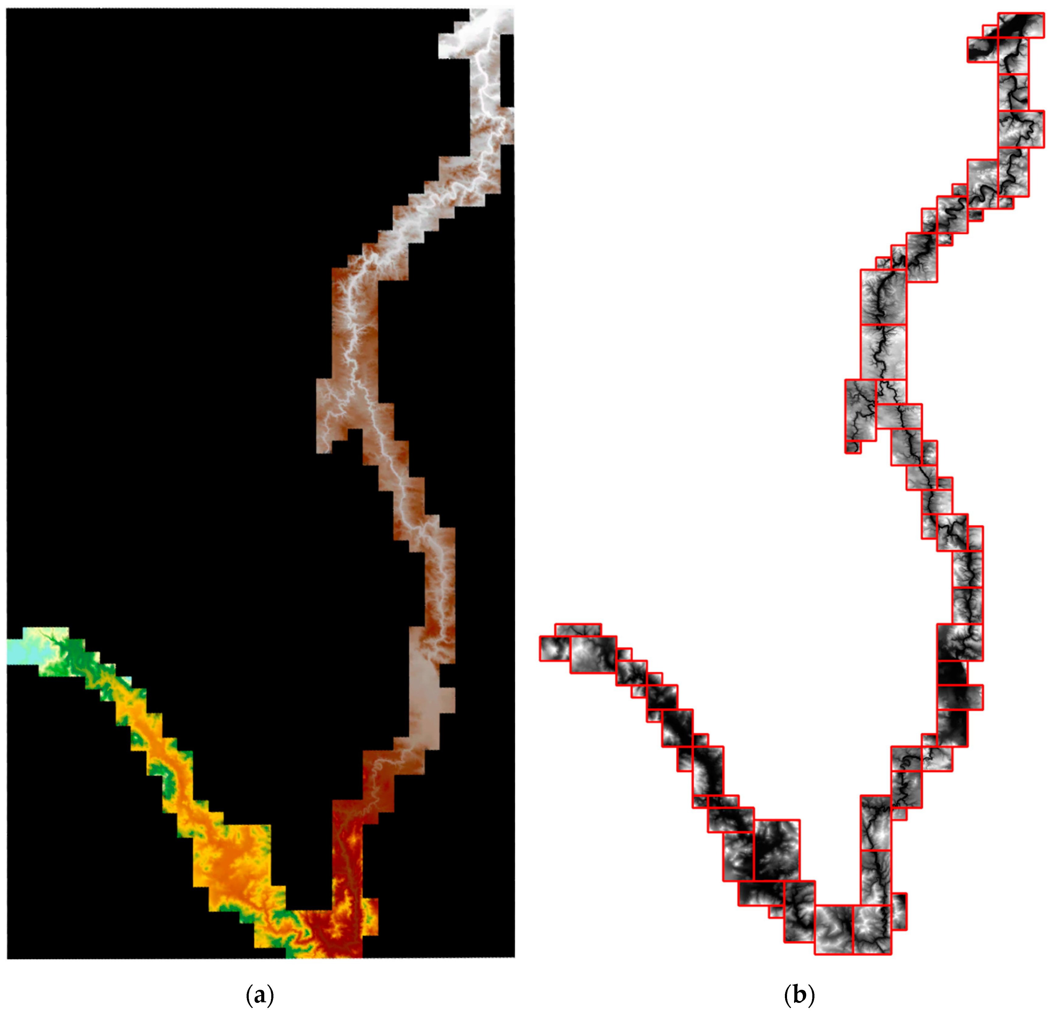
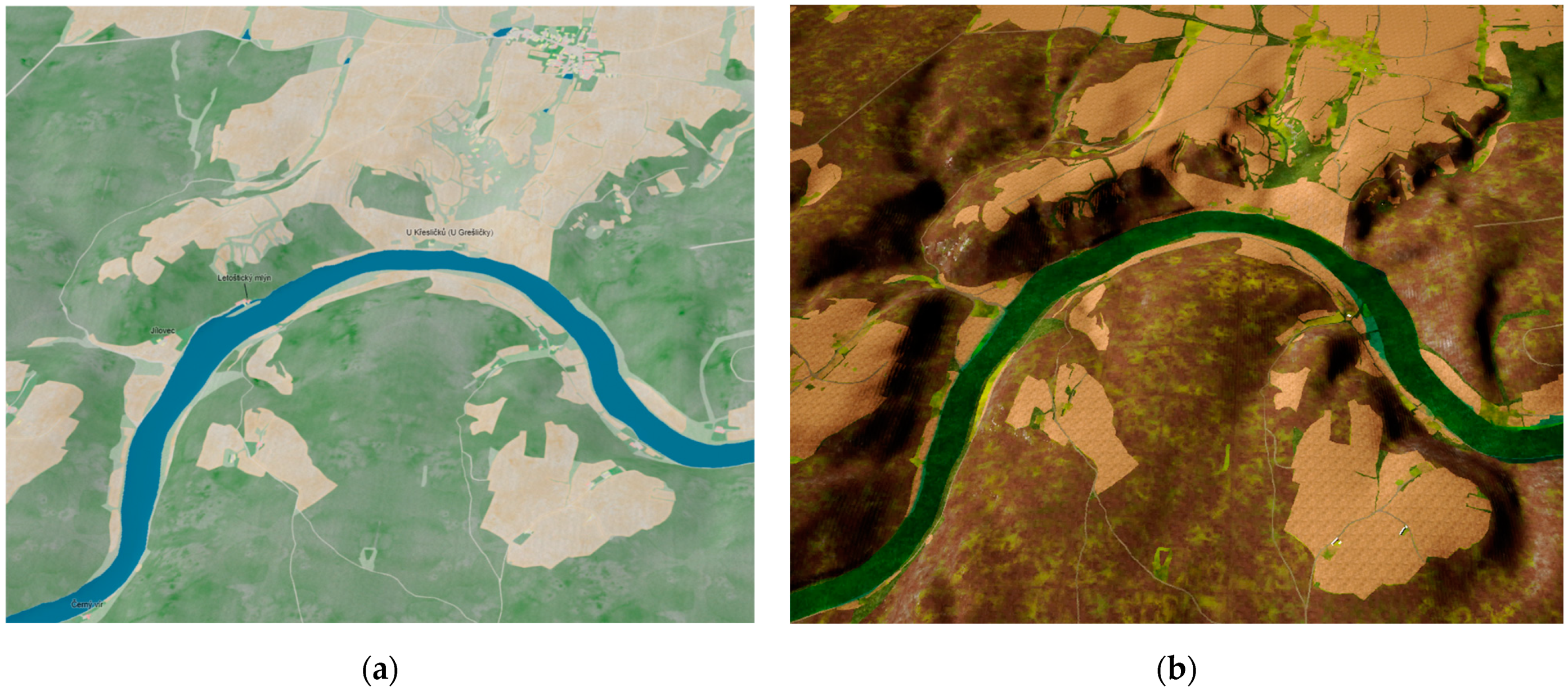
While the DTM raster file containing height data of the terrain can be imported as a single file, reducing the amount of data is necessary to create a more stable and less memory-demanding visualization in UE. As is displayed in Figure 2a, the original one-piece raster contains a large amount of no-data space represented by a black background. This black area is still composed of pixels with their positions and data values. The only difference is that the value is set to zero (or another arbitrary number), which GIS software would identify as such and would not display or use in calculations. This means that even though those areas do not contain usable data for terrain visualization, they still contain data, owing to how the raster data is saved. However, in UE and other non-GIS software, those pixels are taken at their face value, resulting in one big rectangular terrain with a size of over 12,700 km² (as in Figure 2a) compared to the 1670 km² of the area of Vltava valley shown in Figure 2b, and result in terrain being created in locations with no valuable data. This results in UE rendering the 12,700 km² area, significantly reducing performance and increasing hardware demands.

Because of how raster files are saved, the way to avoid empty (black) places is to split the original DTM raster into smaller rectangular rasters, where each raster fully contains part of the area of interest. The area of the DTM of Vltava Valley is primarily created based on SMO-5 maps and follows the shape of the SMO-5 rectangular map sheet layout. The original SMO-5 sheet division was not retained since it would create significantly more individual rasters, which would compound the amount of work needed, since for each terrain raster, there are an additional 14 raster masks of land use information (each land use has its raster: woods, fields, gardens, meadows, pastures, etc.). The division of the original raster into smaller rectangular pieces, which resulted in the creation of 68 individual rasters, is shown in Figure 2b. To divide the DTM, first, an outline of the area containing the Vltava River valley was created using the Raster Domain geoprocessing tool. This Outline was then manually divided into 68 rectangles. The individual rectangles were designed to use as few as possible, but made them similar in size, requiring some larger areas to be further split into smaller rectangles. The aim was to create rectangles covering the whole area, but not containing any areas outside the Vltava River valley. The final rectangles are shown in red in Figure 2b. The next step was to split the original DTM using the Split Raster geoprocessing tool. The resulting rasters were tested in UE, and through an iterative process of trial and error of partially building the visualization, the best parameters for the final raster attributes were found. First, it was found that there needs to be an overlap between the rasters to ensure the continuity of the terrain. However, the overlap should be as small as possible since, in the later stages of the creation of the visualizations, the procedurally created 3D objects like trees may become too dense in the areas of the overlap. Furthermore, due to the follow-up processes performed on top of the terrain, it was decided that the individual raster’s precision (pixel size) should be increased from 5 m to 1 m.

While this precision increase may seem counterproductive in terms of the reduction in memory demands of the visualization, the removal of the empty spots of terrain means the removal of more than 80% of the raster size, and together with the later use of World Partition, more than makes up for it. As is shown in

Table 4. Comparison of DMTs in the context of memory size.

Name	Area of DTM (km2)	Pixel Size (m)	LZW Compression Size (GB)	Uncompressed Size (GB)
Original DTM	12,705	5	0.263	1.89
Upscaled DTM	12,705	1	5.76	47.33
Upscaled 68 DTMs together	1670 +5 m overlaps	1	2.32	6.425
Upscaled 68 DTMs individually	Smallest = 5.07	1	0.00711	0.0193
	Largest = 75.3		0.103	0.287

, while the upscaled DTM takes 25 times more memory due to the increased pixel count, after removing the “no data” background, the size is only 3.3 times bigger than the original. On average, the file sizes of the 68 DTM pieces are in the tens of MB.

This is significant because later in the process of creating the scene in UE, a process called World Partition is used, which renders only objects near the camera/player position. This allows for the dynamic hiding (not rendering) of terrain, vegetation, buildings, and water bodies. However, the content present throughout the scene as one object, such as clouds, sky spheres, or rivers (if not split), will remain rendered. This can be further set for each individual object. This means that only a few of the 68 DTM pieces are rendered at a time, leading to lower memory usage than the single original DTM with a resolution of 5 m. The final 68 DTMs allow further use of world partition (tiling) in UE and, together with the outline polygon, are further used for editing and creating land use data.

Secondly, rasters used for importing terrain into UE through CityEngine should be a 32-bit float pixel type, which is significant information since the rasters used for terrain masks used for applying textures require different pixel types (16-bit unsigned). If the terrain raster had only 16 bit depth, the created terrain in UE would be made of flat pixels resembling stairs, creating an unsmoothed terrain model, which would require either a smoothing pass for the entire landscape in UE or recreation of the imported raster in GIS.

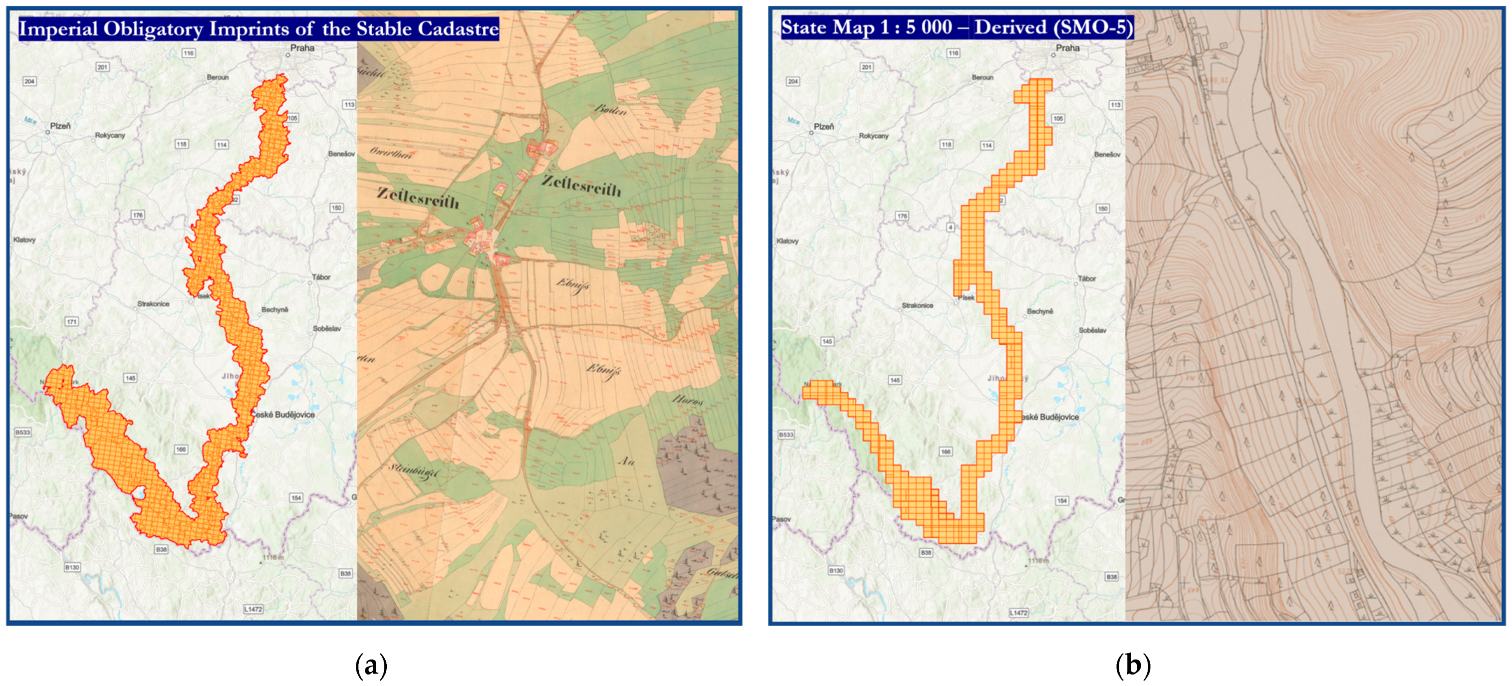
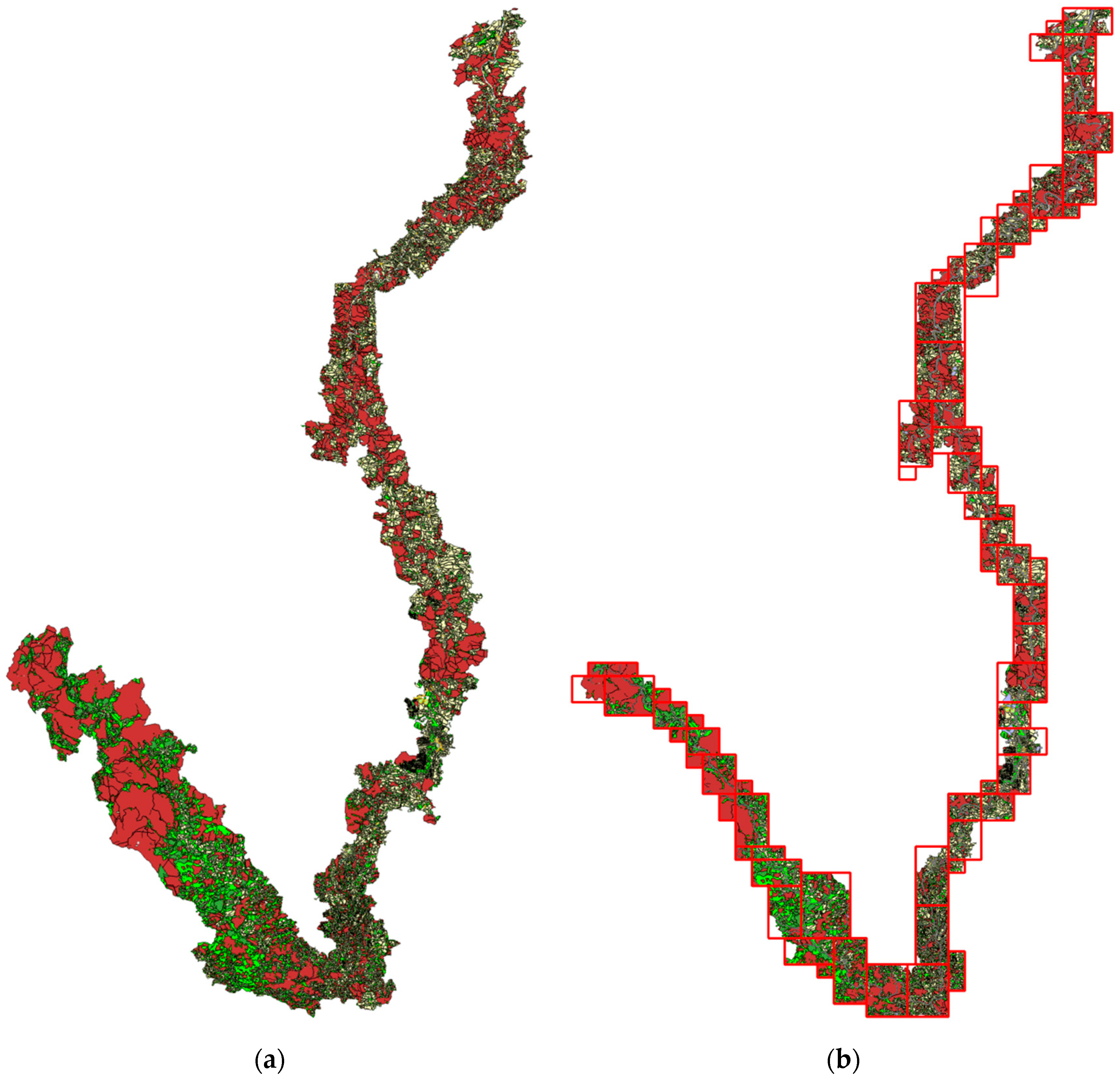
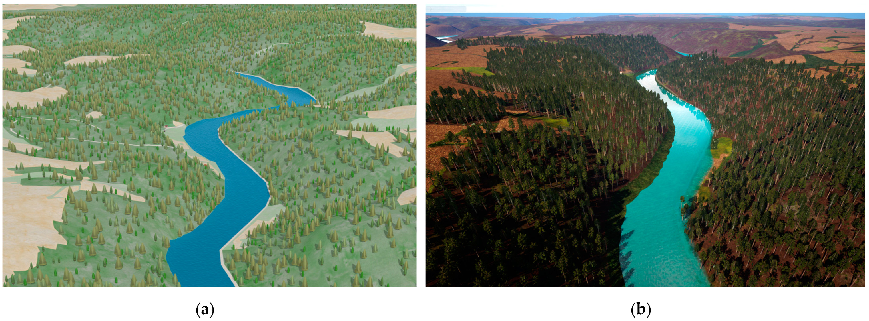
The second dataset was created by manual vectorization of scans of the Imperial obligatory imprints of the stable cadaster, which captures the land use information between the years 1821 and 1840. While in the original GIS visualization, the whole vectorization shown in Figure 3a was used owing to the global height layer available in ArcGIS Online, this layer is not available for use in UE. For this reason, the first change to the vectorization was to reduce its scope to match the area covered by the DTM, as shown in Figure 3b.

This was performed using the Clip geoprocessing tool with the DTM outline polygon shown in Figure 3b as the clipping feature layer. After reducing the land use layer to the area of DTM, the whole vector layer had to be converted to raster. This is because, while the UE can import and display vector data, it converts all polygons into 3D splines. This creates a vast number of actors, which causes performance issues. On top of that, they do not interact with the terrain in any way and cannot be used to visualize land use on the terrain. In comparison, in a 3D GIS scene, 2D layers are projected on top of the terrain, and with the help of Symbology, those layers can apply textures to parts of the terrain according to the land use information. In UE, however, the way to apply textures (in UE, called materials, which on top of textures contain further details regarding physics and lighting-related attributes) is vastly different; terrain (in UE, called landscape) can only have one single material assigned to a landscape. However, this material can be customized using a Blueprint visual scripting system to create multiple layers with different attributes that can be assigned to various landscape parts. This is available as a paint option, allowing manual landscape painting with these layers. However, to use them on a larger scale, an option to import the layer’s area in the format of raster masks must be used. This means that the whole set of land use data had to be converted into a raster form of the exact dimensions of the original landscape, and specific file formats with specific naming schemes had to be used to apply different textures to different areas, depending on the land use information.

Before converting land use data into raster form, it is essential to understand how the final raster is used during UE, so that it can be tailored and changed beforehand. Typically, rasters in UE are used in two ways: to import the landscape itself or to apply textures (materials) using landscape attributes like slope or aspect in raster format. These are then used to apply materials and create seamless material blending between the individual mask layers. The individual pixel values of the mask are either used as a value of fact (for example, slope values) or as a weight for material blending. This visualization uses a process similar to material blending in the importing sense. In this instance, land use rasters in the UE are applied to individual landscape parts as a raster mask. From this comes the first change made to the land use dataset: the aggregation of all separate areas of the same land use under one ID. The goal was to make all regions of the same land use look the same in terms of UE. Since there were no plans for material blending and there is no need for differencing between different areas with the same land use, having different values for each polygon represented in the final raster is unnecessary and may cause problems in UE when applying materials and working with tens of thousands of polygons in GIS (may) cause instability, errors when using geoprocessing tools, and other problems. For these reasons, all polygons of the same land use were aggregated (merged). After aggregating all the values of the dataset by the land use type into fourteen groups using the Select by attribute tool, and merging them, each land use record representing the individual way the land used was converted to an individual raster format, creating 14 rasters in total using the Polygon to Raster geoprocessing tool. However, some rasters, such as water bodies or buildings, were not used further since those were modeled in the final visualization in different ways. Another reason for the aggregation was that using the Polygon to Raster geoprocessing tool with selection as part of the input feature creates one raster for each selected polygon, creating thousands of rasters, which is unnecessary and unsuitable for further data processing.

What needs to be highlighted is the use of the Snap Raster option, which is mandatory at this point of the process because, without it, the output rasters would have different dimensions than the original DTM raster(s), where the areas on the edges of the processing extend may be cut out (for example, because there may not be any forest in the border areas during the creation of land use raster of forests), creating problems further down in the process where the final land use rasters would be difficult if not impossible to correctly align with the landscape in UE during the import of the land use rasters as raster masks.

What needs to be said is that there is a loss of geographic information during the process of converting vector data into raster masks. Although the loss can be reduced by creating rasters with smaller pixel sizes, this is unavoidable. With an area of 1670 km² multiplied by 14 different raster masks, going under a pixel size of 1 m is not feasible due to the sheer amount of space required. This means that details that are less than 1 m will be lost.

After creating the individual land use rasters displaying each land type (forests, fields, gardens, etc.) in this way for the whole Vltava River valley, they were each split to match the rectangular areas of the 68 DTM parts. The process for this further division was very similar to dividing the original DTM using the Split Raster geoprocessing tool. The difference here was the use of the Snap Raster option, where the rasters used for snapping were the individual 68 rasters, to ensure that the resulting land-use masking rasters would match the individual DTM rasters.

2.6. Work inside Unreal Engine

The first step in creating the visualization of the Vltava River valley in the UE was to import terrain rasters as a landscape. This was performed using the Datasmith Importer with CityEngine as a middleman. After the landscape layers were imported into UE and datasets were prepared in the GIS, further preparations on the UE side were necessary to import the land use data as raster masks. Firstly, to correctly display and work within UE, many settings needed to be tweaked/changed to ensure maximal visual quality and functionality of the used processes and, in general, help with creating the visualization both in UE editor and within the final visualization. The most required settings are mentioned further in the text at appropriate places. However, for ease of use and the ability to set everything beforehand, all used Editor Preferences and Project Settings are listed in

Table 5. Used Editor Preferences in UE.

Location	Name	Value
General—Experimental	Procedural Foliage	Enable

and

Table 6. Used Project Settings in UE.

Location	Name	Value
Engine—Rendering	Anti-Aliasing Method	TAA
Project—Packaging	Build Configuration	Shipping
Project—Maps and Modes	Default maps	Select the starting level name
Project—Supported Platforms		Windows
Project—Description	About, Displayed	Fill in information

. The remainder of this chapter describes the steps to prepare for the remaining data to be correctly imported and processed in the UE and the steps made within UE to create the final Vltava River visualization.

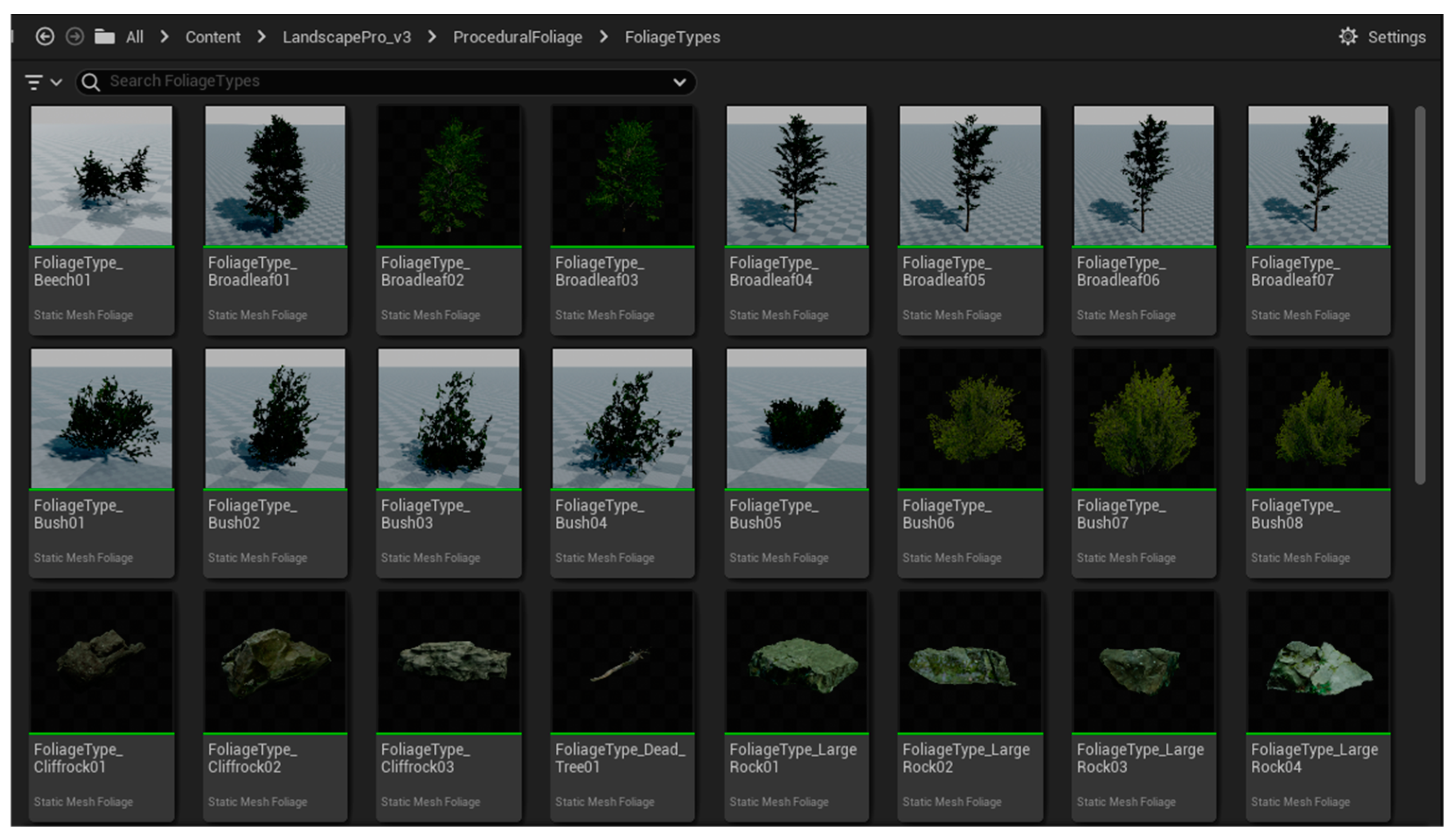
The first step is to display and use the land use data on top of the imported landscape. To do this, landscape layers within landscape material had to be defined. For this purpose, a plugin named Landscape Pro 3 was used. This plugin contains already-prepared materials for the landscape visualization and many textures, 3D models, actors, and other assets, as shown in Figure 4.

These were needed to visualize the land use information and procedurally generate grass, trees, rock formations, and other 3D models based on it to fill up the landscape and make it look organic, realistic, and detailed. 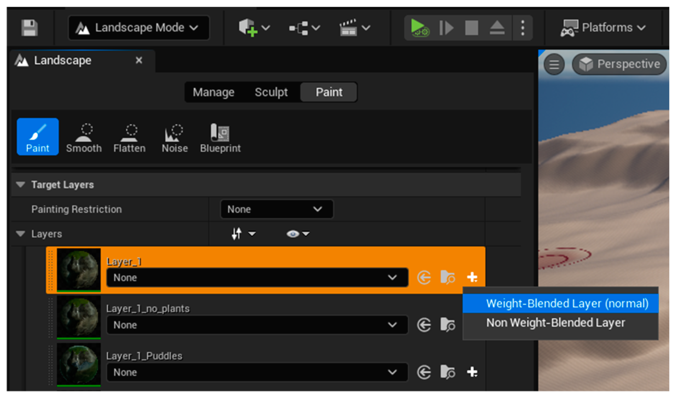After enabling the Landscape Pro 3 plugin, its landscape material was applied to the imported landscape by dragging the material file from the Content Browser plugin directory LandscapePro_v3 > Environments > Landscape to the landscape material attribute inside the landscape actor Details panel. This material file contains the definitions of each material layer, where each layer is composed of parameters, textures, normals, masks, and functions. These layers are then blended to create the final landscape material. Furthermore, this material file contains a Grass Output section that, depending on what layers are blended, procedurally generates ground foliage and 3D objects on top of the landscape. After applying the material, Layer Info must be manually created. To do so, the UE editor needs to be switched to Landscape Mode, and then under the Paint tab, for each layer, Layer Info must be created using the Create Layer Info (the + icon next to each layer) as shown in Figure 5.

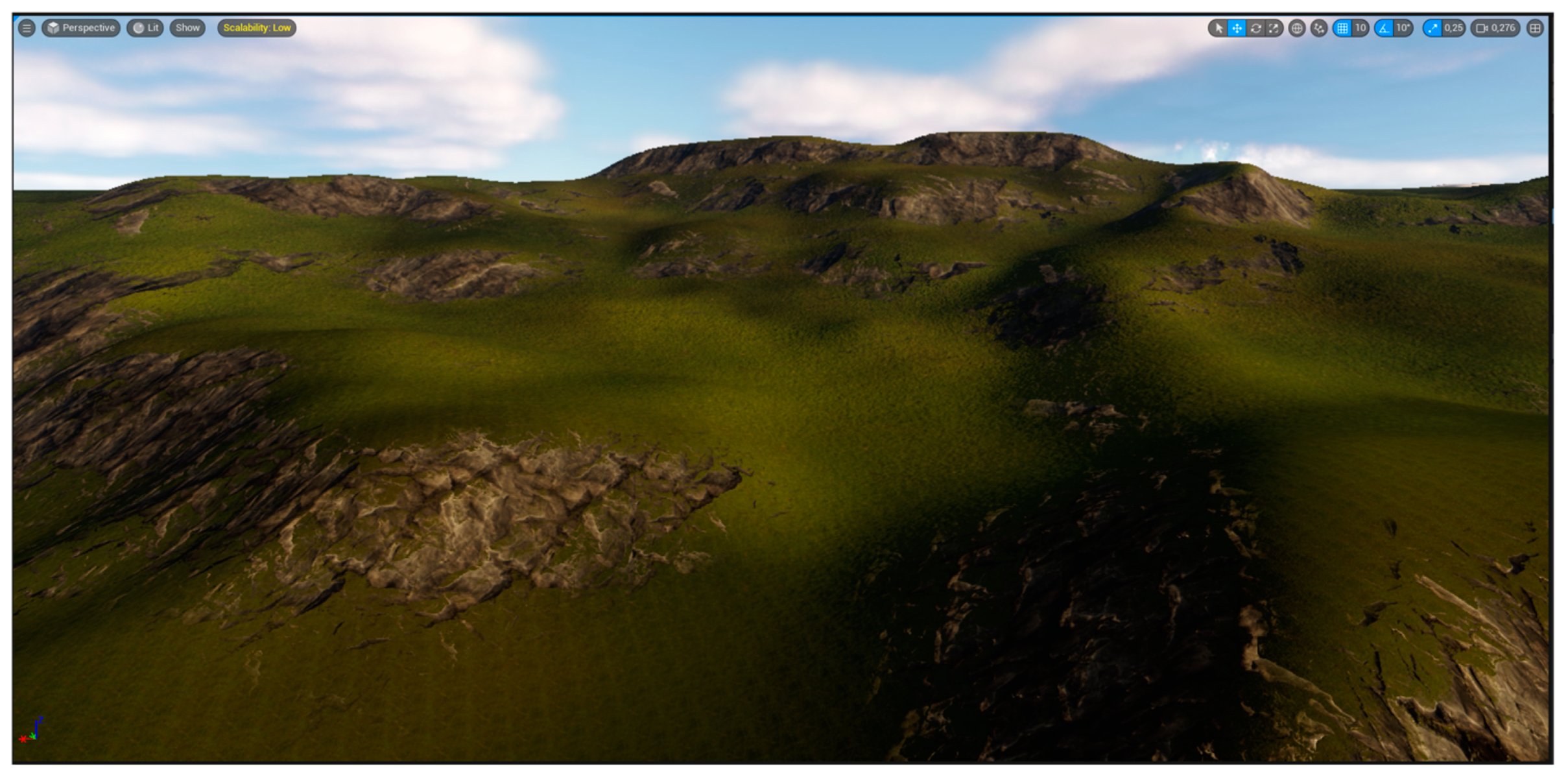
After the Layer Info is created, the base (first) layer will be applied to the selected landscape, which will result in textures being applied where primary terrain attributes like slope are taken into account to apply either rock or grass textures, as shown in Figure 6, together with procedurally generated foliage matching the texture.

Unlike the base layer, all the other layers (from layer two upwards) are not applied automatically and must be applied manually or imported as raster masks. For this, each layer needs its own Layer Info to be created. If a layer is missing Layer Info, the importing feature is greyed out and no import is allowed. The importing of layer masks is located under Landscape Mode in the Manage/Import tab. Each layer with Layer Info allows the importing of raster files as raster masks. Rasters must match specific requirements that are not readily apparent to be imported as layer masks. After all these requirements are met, the rasters can be imported as material layer masks, after which the layers are automatically applied, adding textures and generating foliage and other objects. The requirements are as follows:

The file format of the imported rasters needs to be RAW or PNG

The rasters must have a color depth of 16 bit (greyscale) with unsigned values

All imported rasters need to have unique names within their directory

No auxiliary files can be present in the same folder as the imported raster

Rasters must contain an alpha channel or the file format may not be recognized

Another step in the creation of landscape visualization is to fill it with content. In this case, it is vegetation and its procedural generation. This step is tightly tied to the landscape materials and material layers. The plugin used for their creation also contains procedural generation capabilities. In this case, the procedural generation of vegetation is accomplished in two ways: globally generating ground vegetation and objects on the whole landscape, and locally generating vegetation based on individual land use layers coverage.

The global procedural generation that applies to all the material layers is defined directly within the material layer. It aims to generate vegetation that fills the entire landscape depending on the layers used. The first layer is the base (main) layer for the whole landscape. It does not require location definition as the other layers do and is applied automatically after the material is assigned to the landscape. After the assignment, it applies textures and generates 3D vegetation to the landscape. The generated vegetation consists of small and tall grasses, flowers, bushes, wooden branches, and other ground foliage shown in Figure 7, which is fully animated.

Furthermore, vegetation placement considers the terrain slope and adjusts which and how dense vegetation will be generated. This process is fully automated and does not require any further actions. This base layer can be overlaid at specified locations with the other defined layers, such as layers representing forests, whose locations are imported as land-use raster masks. If the non-base material layers are applied over the base layer, a blend of those layers is created, resulting in the generation of foliage specific to the layers blend, as is defined in the Grass Output part of the material. This feature, however, is not used because of how the original land use data (vectorization created in GIS) was made. It does not contain any overlaps between individual entries, resulting in no possibility of such layers blending in UE outside the base grass layer.

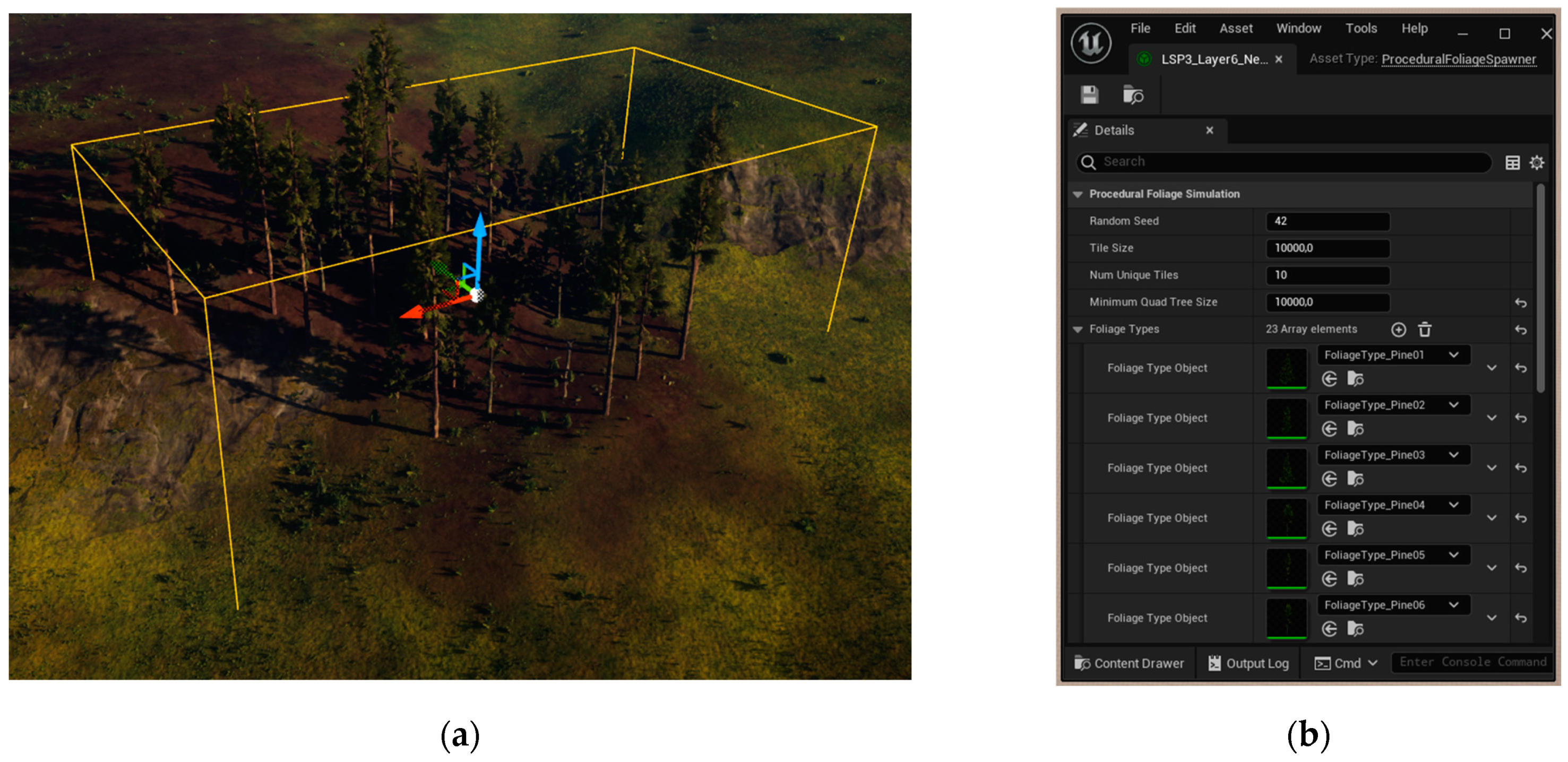
To procedurally generate any of the larger objects, such as broadleaf and needle trees, and rock formations, Procedural Foliage Spawner actors must be used. The spawner creates a bounding box, as shown in Figure 8a, that interacts with specific predefined material layers. This results in procedural generation being performed only on top of the matching material layer and within the bounds of the bounding box. 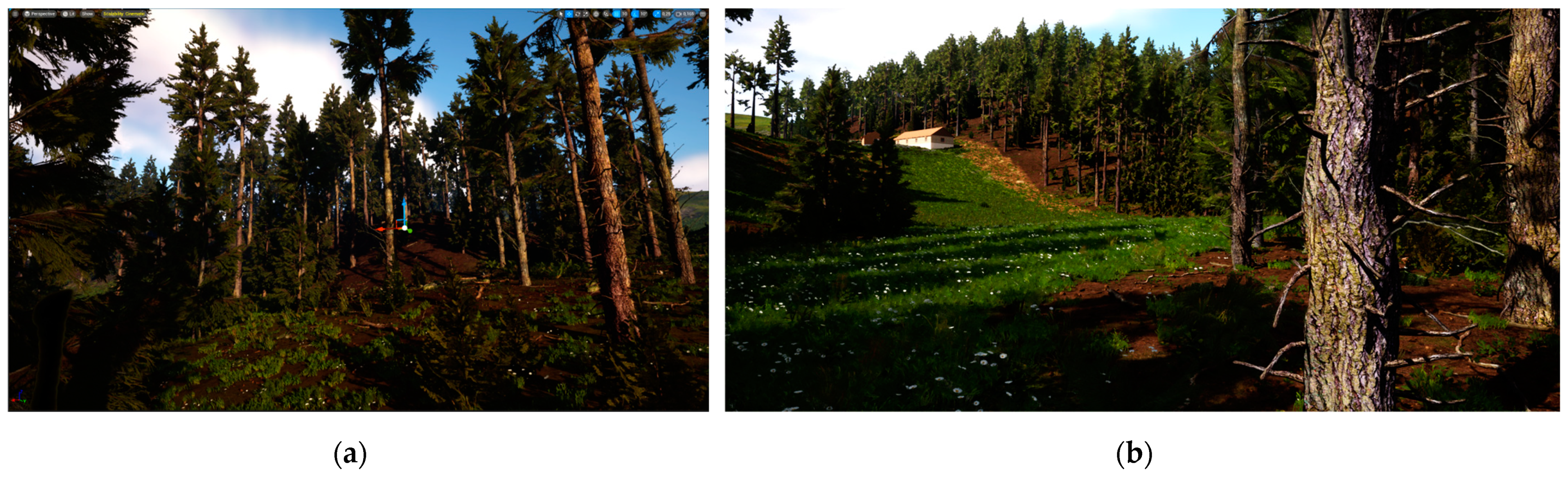Furthermore, the spawner controls which objects will be generated, as shown in Figure 8b. However, the Procedural Foliage option must first be enabled in the Editor Preferences to make procedural generation using the spawners work. Without it, the spawner actors cannot be added to the scene. Another tweaking was performed within the Project Settings, where the anti-aliasing method was changed to Temporal Anti-Aliasing (TAA) to remove flickering and shimmering effects from the animated foliage to create organic, realistic, and detailed foliage, as in Figure 9.

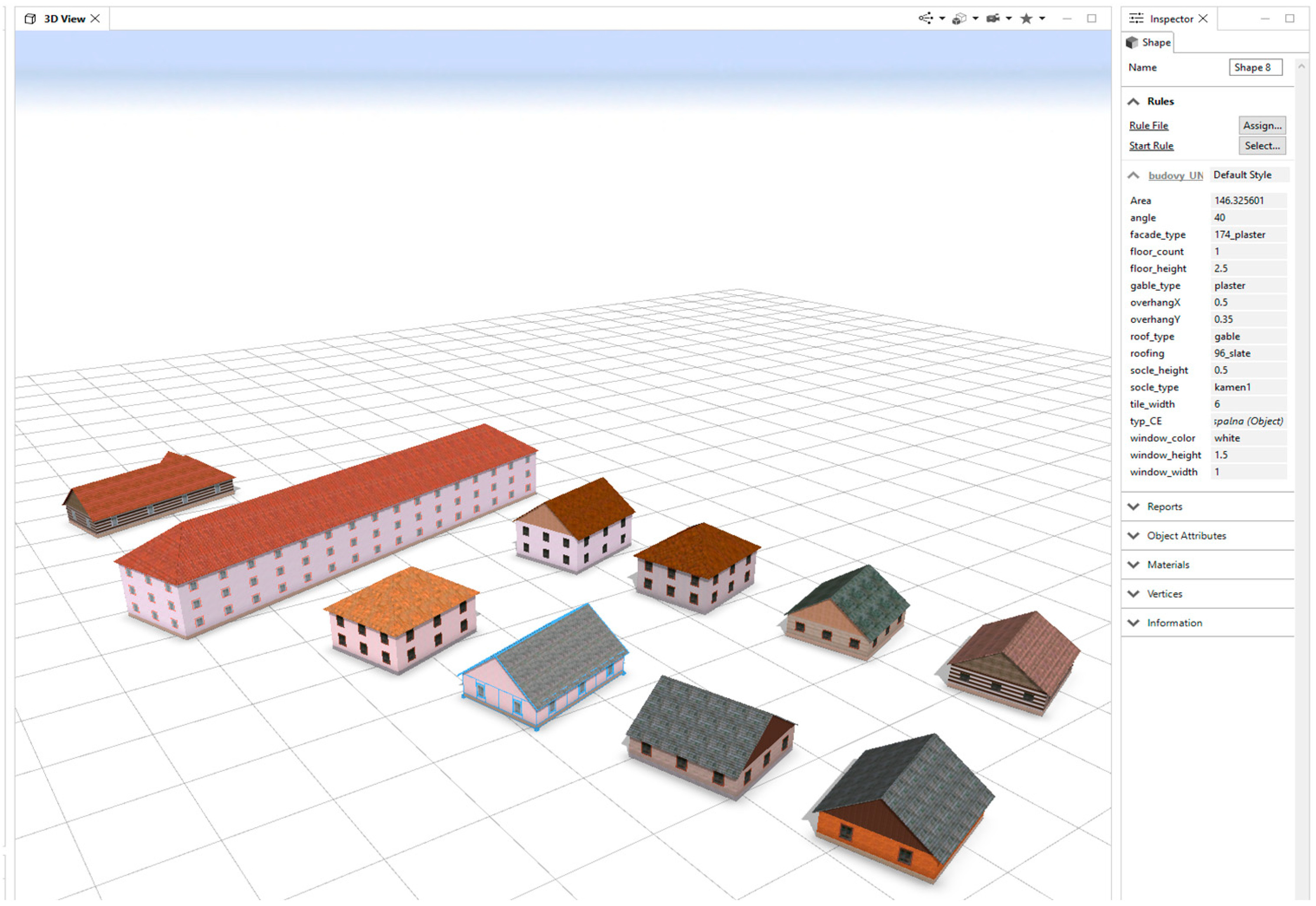
The primary method of creating 3D models of over 28,000 buildings was procedural modeling performed in CityEngine, as shown in Figure 10. However, these are not part of the input data for this case study since those models were only exported in a format compatible with ArcGIS Online at the time of their creation. Since one of this study’s goals is to recreate the Vltava Valley’s visualization, recreating those 28,000 models is also needed. The easiest way to create these models again is to use CityEngine and import them, either in the *.udatasmith format or any other format supported by UE (for example, glTF). However, because the case study aims to explore the usage of GIS data within UE, another solution has been used.

CityEngine is a 3D modeling software locked behind a license, but it has a freely downloadable software development kit, CityEngine SDK. This C++ API allows for implementing procedural modeling, as is used within CityEngine. Based on this SDK, a plugin for UE was developed, named Vitruvio. Vitruvio is free for personal, educational, and non-commercial use; however, as an input, Vitruvio requires Rule Packages (RPK), which are created in CityEngine and require a license [34,35]. While using Vitruvio, the procedurally created buildings remain procedural and can be changed easily with a parametric interface (height, style, and appearance). An RPK file includes assets and a CGA rule file that encodes an architectural style.

To use Vitruvio, polygons that represent the footprints of the modeled building must be imported into the UE. This is completed using CityEngine and the Datasmith Importer. This creates Actors for each imported polygon in the project. Once the polygons are imported, a new action menu option will appear: Select all viable initial shapes in the hierarchy. This will select all Shapes within the selected Actors, which can then be converted into Vitruvio Actors with the procedural modeling functionality. Before conversion into the Vitruvio Actor, the RPK file must be present within the project. To do so, the RPK file created in CityEngine must be dragged into the Content Browser. After selecting from the context menu, Convert to Vitruvio Actor and select the desired RPK file. All shapes will be converted to the Vitruvio Actor, and the original polygon will be modeled into the desired shape according to the RPK file, which, in this case, will be fully textured models of buildings.

3D modeling of over 21,000 buildings was quick and took a couple of minutes on both tested machines. This is comparable with procedural modeling performed in CityEngine. The process was also stable during testing, and repeated importing and procedural modeling were performed on both tested machines. After converting Shapes into Vitruvio Actors, it is possible to change the attributes used for procedural modeling using the Vitruvio Actor details inside the Vitruvio Component section under Attributes. The implementation is similar to procedural modeling in ArcGIS Pro, which is available under polygon symbology as an option under the fill symbol layer. Both methods use CityEngine RPK files to create models procedurally based on the polygon footprint. In both cases, each will have its attributes created based on the rule file that is part of the RPK. These attributes can be changed to edit the look of individual models. Neither of these implementations (UE or ArcGIS) allows for creating or editing the original rule file or alerting the original assets that are part of the RPK, which is limited only to CityEngine, in which the rule file was created. The UE version also contains more options related to physics and materials that are unique to game engines.

The last unique step for the UE is the conversion from Vitruvio Actors to Static Mesh Actors. This process preserves the changes made to Vitruvio Actors and saves procedurally modeled objects. Without this conversion, Vitruvio Actors would continue to exist until the project’s closure, after which they would cease to exist, and the original shapes would need to be imported again. During the conversion of Vitruvio Actors to Static Mesh Actors, a process of so-called Cooking is used. UE stores content assets in particular formats that it uses internally, such as PNG for texture data or WAV for audio. However, this content needs to be converted into different formats because the platform uses a proprietary format, does not support Unreal’s format used to store the asset, or a more memory- or performance-effective format exists. The process of converting content from an internal format to a platform-specific format, together with compiling shaders, is called cooking. This process can take longer with more complex assets (like meshes with lots of polygons, etc.) [36]. This process is conducted in the same way as the initial conversion, meaning that after selecting all Vitruvio Actors in the context menu, there will be a new option: Convert to static mesh actors. Unlike procedural modeling, this process can be volatile due to its very high hardware (memory) requirements, and the time needed is also severely longer, where finishing these conversions takes hours. Solutions to these problems are to split the number of Actors processed at a time into smaller chunks, in this case, 10,000 at one time, or to increase available memory either by installing more RAM or significantly increasing the size of the system’s virtual memory via increasing the page file size in Windows.

During model cooking, the CPU and memory are utilized significantly. While the CPU speeds things up, insufficient memory leads to a UE crash. Resource Monitor reveals that UE commits over 170 GB of memory just for itself at the time of cooking.

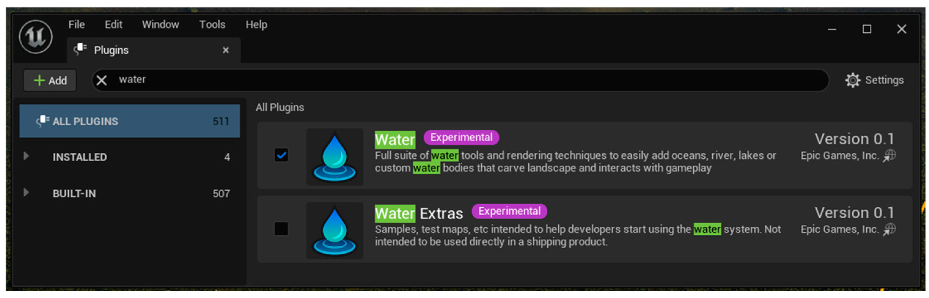
Another part of the visualization is creating water bodies. To add and work with water, a plugin of the same name, Water, is used. This plugin is built into the UE and is currently in the experimental version, as shown in Figure 11.

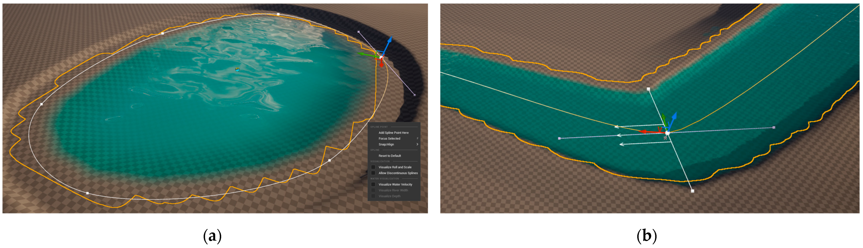
This plugin brings multiple types of water bodies to the UE. Still, only two are being used to visualize the Vltava Valley: Lake for modeling smaller water bodies like fish farms, water reservoirs, or ponds and River for modeling the Vltava River and smaller streams, as shown in Figure 12.

The simpler of the two is an Actor named Water Body Lake. This actor creates a lake defined by three Spline points with the possibility of adding additional spline points. These spline points are connected by arc-shaped curves whose attributes can be changed using the detail panel or graphical representations of these attributes directly in the editor scene. This actor is more straightforward than a river because a lake has only one height value (the lake must be flat). Specific attributes, like the speed of water flow, do not matter for small-scale water bodies, and there are significantly fewer attributes in general. By default, the lake actor contains the attribute option Affects Landscape, which allows the lake to interact with and change the landscape on which it is situated. While this feature can be disabled, it must be used since the smaller water bodies for which the actor Water Body Lake is used are not modeled within the DTM. In the original datasets, they are represented only by land-use vectorizations and consequently by texture (only their position is known). The lack of lake bottoms in DTM and their representation only in vectorization create additional problems. Since many water bodies contained in the land use vectorizations are made of sharp angles, which are significantly harder to achieve using the spline points, it is lengthy and complicated to perfectly match the position of the banks with the vectorization. Furthermore, the exact measurements of the bottom of these water bodies (depth, angle, etc.) are unknown, at least in the datasets used for this modeling. This results in higher creative freedom in how the water bodies are created; however, it is at the cost of historical accuracy and the accuracy of following the base GIS data, in this case, the vectorization of old maps.

The actor named the Water Body River is a more complex one. Like the lake actor, it creates a river defined by multiple spline points; however, these have many more associated attributes. Firstly, each spline point has its height (Z coordinate), making the manual creation of rivers more accurate but at the cost of the increased difficulty of working with the river actor. Furthermore, each spline point has its depth point, river width, flow orientation, and flow strength/speed. The actor Water Body River also contains the attribute option Affects Landscape; however, in the case of the Vltava River, the situation is reversed. Since the used DTM already includes the bottom of the river basin, there is no need to alert the terrain. Furthermore, doing so could lead to terrain continuity problems, where it could/would be challenging in specific spots to make the terrain changes made by the river actor unnoticeable and seamless with the original terrain. Another reason for not using the Affects Landscape option is that, by not using it, the whole workflow of creating rivers can be significantly simplified. Since the water level is always lower than the surrounding terrain and the bottom of the river is already modeled within the DTM, these attributes can be made purposefully larger to fill the river basin. This reduces the whole process of creating the river by removing the need to set up each single spline point with depth, width, and terrain angles to only create the individual spline points and set their location, which is already a significantly lengthy process considering the shape of the river and its length and the fact that the spline points are all created and positioned manually. However, a combination of both Affects Landscape options is used for creating streams according to individual stream locations and the terrain around them. Since these streams are substantially smaller than the Vltava River, using the Affects Landscape can help highlight the stream in the terrain. This is especially welcomed when physics-abiding water in the UE would not be usable to create such streams because of its location on flat or sloped terrain. Similar to the situation with lakes that are not modeled within the DTM, the position of the stream bed may not be modeled in the DTM. In certain instances where the stream is, for example, in the ravine, this may not be a problem, but a stream going through pasture or meadow may require the use of the Affects Landscape option not only to make the stream stand out, but also to be able to model the water correctly.

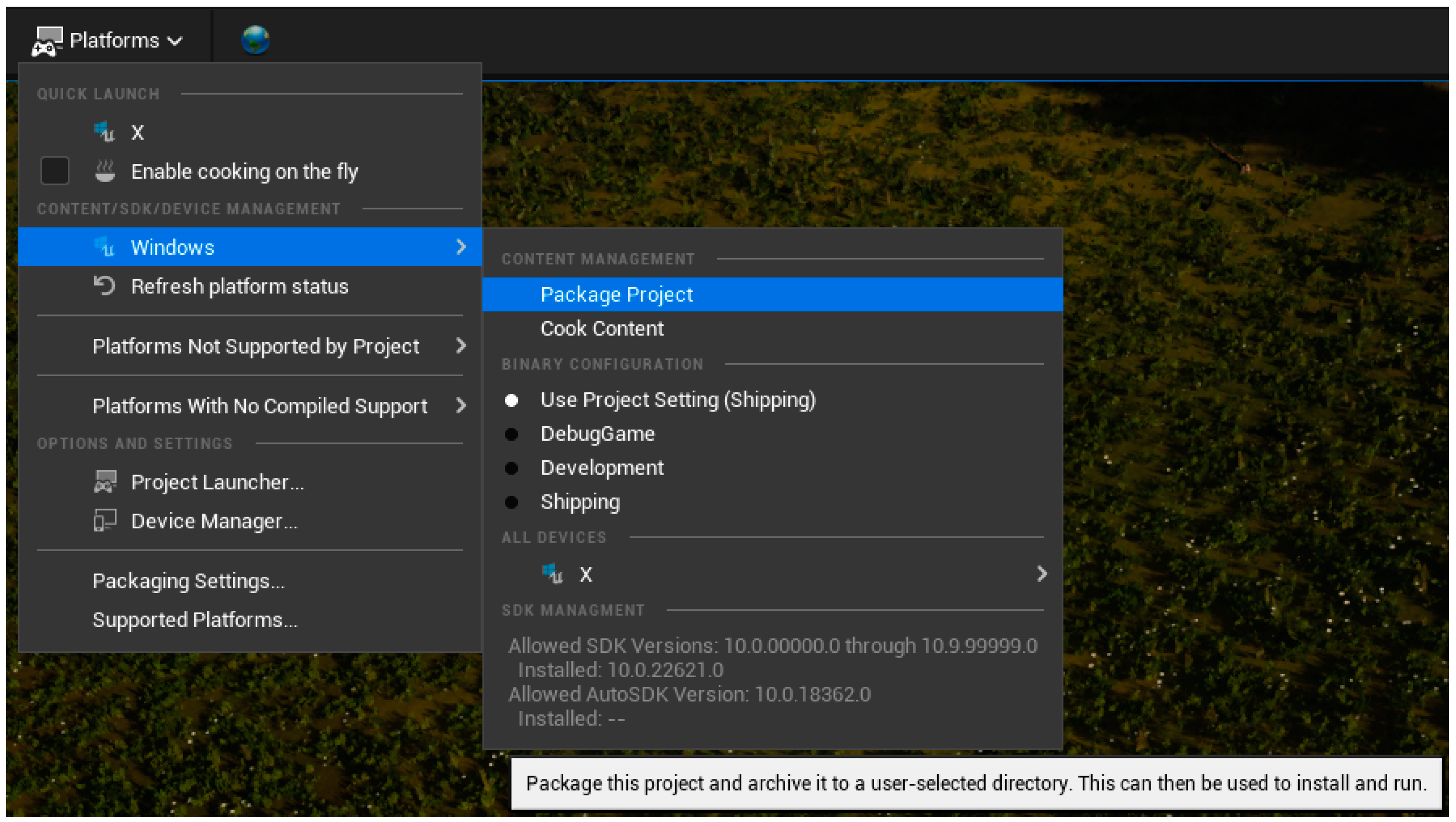
After the scene is filled with content, meaning it contains the finished landscape with applied material layers according to the land use information, with procedurally generated vegetation on top of it, all the water bodies, and the procedurally modeled buildings, the last step is to package the whole scene. Packaging a project is the final step, which allows the scene to be opened via an executable file and no longer requires UE to be installed. The first step in packaging the project is to fill out all the information in Project Settings under ProjectDescription, namely Project Display Title (also used by the operating system), publisher information if applicable, project version, and others. Next, choosing default maps (levels) to be opened in the Project—Maps and Models section is crucial. Lastly, the Build Configuration needs to be set to Shipping in the Project-Packaging section, allowing the opening of the final packaged project without needing UE. All other settings can be changed according to an individual project’s needs; however, they are left with default values for this study. After the project is set up for packaging, it can be selected from the main toolbar under the Platforms, as shown in Figure 13.

However, this step has an excellent potential to cause errors and failure. The most straightforward errors to solve are those related to the required SDKs, which can be fixed by installing and updating.NET Core 3.1, .NET 9.0, Windows SDK, and Visual Studio 2022. Another set of problems may arise from the deleted and unused content within the project. The packaging process packages all levels, including any (testing) unused levels. The problem is that they usually contain invalid references to deleted content, which will cause packaging to fail.

For this reason, it is essential to “clean up” the whole project before packaging, for example, using the Content Browser filtering option Not Used at Any Level. After all these steps are completed and potential errors are resolved, the project packaging process can be completed. It is important to note that the entire packaging process takes a significant amount of time and fully utilizes the computer CPU for compiling shaders and packing the project per the chosen options in ProjectPackaging within the Project Settings. After the packaging process, the application executable file and all packaged assets are created within the selected folder. This application opens up the previously set default level for the created visualization with basic movement and camera controls. Within the application, no further modifications to the visualization can be made (outside of programmed interactions); however, the project within UE can still be used and worked on, and a new version of the application can be packaged.

3. Results

This case study provides information that is usually missing for similar projects. It describes the used GIS data, its origins, used software and plugins, and delves into the recreation of the 3D visualization of the Vltava River valley in Unreal Engine in detail with a focus on practices for importing and processing GIS data in UE, techniques for creating realistic-looking scenes as shown in Figure 14, performance optimization techniques for ensuring a seamless viewing experience, possibilities for sharing and/or publishing of the resulting visualizations, and lastly by focusing on the workflow of 3D visualization in general. Furthermore, the results of this case study compare the individual parts of the visualization process, requirements, and suitability with the visualization created as part of the Vltava project using GIS software. This allows readers to understand better what processing and visualizing GIS data in UE entails and how it compares with GIS so that they may gain the basic knowledge to start creating visualization works in UE.

3.1. Summary of the Visualization Workflow

First, before any attempts to create the visualization in UE were made, the question of importing GIS data into the UE had to be answered. For this purpose, multiple ways to import GIS data were tested and discussed. While each way to import data has pros and cons, importing using CityEngine was used.

This method allows the import of all required GIS data types (3D models, rasters, landscape splines, etc.) with correct coordinates and relative positions to each other. This was the major problem with importing solutions using plugins, where the importing process transformed the data, which caused data types that were unsupported by the individual plugins to be imported separately.

After importing the first GIS datasets, the process of creating the Vltava River Valley visualization began by trying to work with all the unedited GIS datasets and using an iterative process of trial and error to progress further with the creation of the 3D scene in UE. Each hurdle in this process was then documented and, in many cases, resulted in the need to edit the base GIS data in GIS software to better suit the UE’s needs. The changes to the original GIS data can be summarized as optimization and functional changes. Optimization removes unnecessary data and primarily reduces memory usage in UE, while functional changes make the GIS data usable for use in UE.

The next part of the article aims to describe and explain each step required to create a basic visualization of the Vltava River valley. It began with the problem of using GIS vector data as a source of information for applying textures to the terrain in UE. In GIS, this is performed by simply projecting polygons onto the terrain with their symbology. However, the UE does not work this way. Instead, polygons must be applied as raster masks directly to terrain rasters. For this reason, the precision of these rasters had to be increased to allow smaller areas and details in the vectorization not to be lost during the conversion from vector polygons to raster pixels. These raster masks were then used for procedural modeling of vegetation using the plugin’s material. Another step was to create models of more than twenty thousand buildings by importing vector footprints and procedurally modeling them in UE via a plugin Vitruvio (based on CityEngine SDK) to test the plugin’s functionality and avoid problems with importing models.

One part of the visualization process is vastly different from the others: the creation of water bodies of rivers, lakes, and streams. Unlike the other parts of the visualization, which were at least partially automated, the water bodies were all created fully manually using the built-in plugin Water. This is the only part of the visualization that does not precisely follow the underlying GIS data. While there was an effort to follow the available underlying GIS data, due to the limitations of the manual creation of the water bodies, in many places, an approach based more on the visual aspect of this visualization was used, where the water line followed but did not fully match the original land use data. Furthermore, during the visualization process of some water bodies, the terrain had to be altered and remodeled since the DTM data were incomplete and did not contain the bottoms of water bodies like lakes.

The last part was the creation of an application that contains the visualization of part of the Vltava River valley outside of the UE editor. This was accomplished using project packaging with default settings for flyover controls. This was ensured due to the upcoming plans for this visualization to be used as a basis for further applications such as VR or prerecorded animations, which don’t use traditional controls (animations) or require specific hardware (VR).

3.2. Comparison of GIS and Unreal Engine Visualizations

One of the arguments for recreating Vltava River visualizations in UE was the possibility of achieving more realistic graphical fidelity. For this reason, this section contains image comparisons representing the resulting visualization created as part of the case study in Unreal Engine and images from the original GIS visualization from the exact locations, focusing on individual content types (terrain, vegetation, buildings, and water). For each of these comparisons, an explanation of the differences is provided.

The most basic comparison comes in the form of a distant view of the broader landscape. Figure 15a shows the final GIS visualization hosted on the project Vltava website. This GIS visualization uses bright colors to differentiate between different land use areas and lacks any form of shadow due to the static lighting directly above the scene. While this can be changed inside ArcGIS Online, the final visualization hosted on the project’s website does not have this feature. On the other hand, the image from UE uses more realistic textures, which are noticeably darker, and uses dynamic light that helps to define the terrain, as shown in Figure 15b.

While from the air, those visualizations look very similar; upon moving closer to the landscape, this changes drastically, as shown in Figure 16a. In GIS, the trees are simpler and behave differently in terms of LOD. In GIS, these trees use a simple model without regard to the distance rendered; however, density changes based on distance. On the other hand, in UE, the density remains the same, but the model changes based on distance, as shown in the second image of Figure 16b. The LOD in UE can be split into three levels: The closest trees have full details and shadows, trees further away are simplified and have the shadows removed, and trees in the far distance are removed.

In GIS, outside of the trees, which are disabled in the visualization by default, there is no other form of foliage or vegetation, and in general, GIS visualization is not optimized for up-close viewing. This is showcased in Figure 17a, where bare ground without any ground foliage and the pixelated division between two areas (forest road and meadow) can be seen. However, the UE visualization in Figure 17b is covered with details that are better suited for viewing from up to close.

While there is currently a problem in UE with distinguishing the borders between areas because of the use of rasters as raster masks for applying textures to the landscape, which may be apparent in specific situations, blending between neighboring areas is an advantage in others.

In terms of building models, there are only minor differences. From the above, the buildings seem the same, but up close, the models look better in UE, even though they are the same models created in the same way. This is showcased in Figure 18. The cause of this sudden upgrade in quality is unknown. However, a better rendering technique, shaders, shadows, or lighting may play a role. The only downgrade to the building models in UE comes in color due to different light settings, exposure, and texture attributes in UE.

4. Discussion

During the literature research, it was found that the majority of projects that visualize large landscapes (small projects workflow is unsuitable for large projects due to the differences in approach to optimization, unreasonable levels of manual work, hardware requirements, etc.) that were found during the literature research provide little or no data and data processing procedures and focus primarily on the introductory information and images of the final visualizations, which were shown on two large projects, creating a gap in the literature regarding the data processing process. This is a significant problem, as other researchers cannot validate the procedures used or suggest improvements. Furthermore, new researchers starting with game engines have never adopted already proven procedures. A case study was created to help bridge this gap and find more information to answer each research question.

4.1. Comparison with Other Projects

4.1.1. Rome Reborn

Rome Reborn was an ambitious project, currently version 4.0, that aimed to digitally recreate the ancient city of Rome as it appeared at various points in history [27]. However, only the first half is somewhat documented before the project changed course and became a closed-source paid product with version 3.0 in 2019 [37].

In the first versions of Rome Reborn, which formed the basis of its visualizations, various software tools were employed, including 3D modeling software such as 3DS Max and Maya, and procedural modeling techniques using CityEngine. Similar to the Vltava project, buildings were split into two categories: one was precisely modeled using 3D modeling software, and the other (made up of primarily common houses) was created using CityEngine. Ref. [24] CityEngine is a significant help in modeling buildings for which only basic information is known. Furthermore, procedurally modeled buildings are often of low importance, but in large quantities, manual modeling using CAD or 3D modeling software is highly time-consuming.

In terms of scale, it is safe to say that the visualized area was smaller than that in the Vltava Project and smaller than the attempted scale of this case study. Rome Reborn focuses on an urban area with a high density of buildings (7000) and a high density of significant buildings (250) [24]. In this case study (under the Vltava project), even though the visualized area is mainly composed of rural areas with large quantities of dense fields and forests, it has more procedurally modeled buildings (over 21,000), although in significantly less detail.

The use of game engines, namely Unity, came in Rome Reborn 3.0, which means practically no information on what and how has been performed in Unity, which causes a significant gap in the literature regarding this project. From the available images and the project webpage, it can be deduced that many assets from previous project versions were imported. At a minimum, a VR application was created for virtual tours that are now offered for sale. However, due to this lack of transparency, any new DOI-issued articles regarding Rome Reborn after version 3.0 was released only contain basic descriptions of the project and the virtual tours [25], so much so that as a source of information for any other project, they are useless and only serve as adds for the sale of the virtual tours. This is probably the most significant difference between Project Vltava, within which the results of this case study are freely available. This study aims to provide as much information as possible regarding using the UE as a visualization tool and to bridge the literature gaps created by projects like Rome Reborn that only show what is possible but not how.

4.1.2. Virtual Angkor

Virtual Angkor is another significant project that aims to reconstruct the ancient city of Angkor in Cambodia digitally. While not all information regarding this project is public, compared to Rome Reborn, significantly more information is available. The project’s goal was to create a virtual representation of Angkor during its peak period in the 12th century and showcase the architectural wonders of Angkor Wat, the Bayon Temple, and other iconic structures, as well as the elaborate urban infrastructure and water management systems that characterized the city at that time [22,38]. Virtual Angkor created three main applications.

First, the area of Greater Angkor (3500 km²) was visualized using a GIS-based solution that incorporated LiDAR data, DEM, and GIS mapping layers. Furthermore, a significantly smaller area of Angkor Wat (the exact area is not defined, but from available sources, the estimate is around 2 km²) was visualized using the Unity game engine. Like many other projects, including Vltava, the Virtual Angkor began with works outside game engines that were later imported into Unity to transition away from 3D scenes built to render single images and animated sequences. This approach of visualizing large areas in GIS and smaller areas in more detail using game engines was also utilized in the project Vltava. However, this case study aims to recreate the whole area in Unreal Engine, which is used to evaluate and highlight the scalability of UE in terms of the visualized area instead of highlighting the depth of the possibilities of the game engine, such as is showcased in the Angkor Wat Unity scene.

Second, Virtual Angkor capitalizes on the sheer number of game engine capabilities. It creates a profoundly detailed simulation of Angkor Wat with fully animated and living characters going through their daily routines. While neither this case study nor the Vltava project has the ambition of creating a simulation of living beings, it highlights the capabilities of game engines.

Third, virtual reality is one of the primary forms of visualization for Virtual Angkor. It provides intractability and allows users to immerse themselves in the fully simulated area of the Angkor Wat. While a VR application for the project Vltava is likely to be created in the future, it has not been created for the current case study due to the sheer amount of work with the base visualization, which needs to be completed first.

Sadly, even though the Virtual Angkor project provides a lot of basic information, it is still not valid as a source of information for any other project to follow in its steps. Once hosted on the official project website (based on multiple archived internet articles referring to it), the official GIS-based interactive map has been stripped away. Furthermore, the official website contains only descriptive information with no indication of any workflow that could be followed, either for recreating the GIS-based interactive map or the simulation in Unity. Next, the sources listed on the project website are tied to the area, but it is not stated that they are related to the project. The only things that stand to interest on the project website are teaching modules, which do not provide information on where they are deployed or how they can be obtained for education and 360° video views. Sadly, this approach of locking everything from public access and not even providing basic workflow or some other way to share the research behind those projects further aids in creating a literature gap, where new research is purposefully gated by the lack of usable documentation from similar research.

Yet again, the most crucial difference for the further development and usage of game engines is the aim of this study, which is to provide as much information as possible regarding the use of the UE as a tool for visualizations and to bridge the literature gaps created by projects like Virtual Angkor that only show what is possible but do not show how.

4.1.3. Virtual Scene of Poyang Lake

A case study of Poyang Lake proposes a workflow of game engine-based virtual wetland scene construction for the rapid modeling of virtual wetland scenes. The visualized area averages 3500 km² (depending on the season) and consists mainly of the wetlands of the Poyang Lake [21]. Compared with the Vltava case study, the visualized area does not contain buildings, trees, or area-wide grass coverage. Instead, the region is comprised of wetlands, specific grasses, and plants. While this may not sound like a big difference, considering that a large part of the area is filled with a lake (deep water without any foliage modeled), this results in significantly lower performance required and thus allows visualization of an even bigger area than in the Vltava case study, and as such can be used with a less powerful PC.

In the lake study, UAV-gathered data were processed into information about the wetlands to create an informational basis for setting individual material layers. Information such as soil type and height above or depth underwater level is used to determine which layer with what weight will be applied and blended. It is then used to generate specific types of grass or plants [21]. The Vltava case study uses a similar process of assigning material layers for slightly different purposes. Land use information from vectorized old maps is used as the basis for applying material layers, which are used for the procedural modeling of buildings and the procedural generation of vegetation.

The lake study uses various virtual reality solutions and technologies to display a virtual wetland scene and realizes multiple forms of virtual experience. One such solution is hosting the visualization online through WebVR and HTML. This is an interesting choice since the lake study was published in 2023. However, the support for rendering to HTML has been deprecated and removed from UE with the update 4.24, released on 9 December 2019. While the possibility of hosting the visualization from the Vltava case study on the project webpage sounds enticing, since the Vltava study is made in the newer UE version (5.2), it would require downgrading and porting of the content, which may be significant work, not to mention problems with used plugins and their compatibility issues.

The other VR solutions in the lake study include a standard head-mounted display and a CAVE (Cave Automatic Virtual Environment). While a standard headset VR implementation is planned within Project Vltava, the case study focuses on the visualization’s construction.

In conclusion, the case study of Poyang Lake, while having different goals and using different types of data, uses similar techniques that achieve, in theory, the same results. To automate the process of placing objects in the visualization, in the case of the lake study, it would be wetlands-specific plants, and in the case of the Vltava case study, it would be general foliage and vegetation; both studies utilize material layers. While in the lake study, those layers are based on terrain attributes obtained from UAV scanning, such as soil type, terrain angle, and height (depth), the Vltava case study obtains those layers as terrain uses information obtained from vectorized maps. The major difference between the two is in the resulting forms in which visualizations are presented. Currently, the Vltava case study only creates a PC application with a VR application planned for later, while the Lake study provides only VR applications for multiple VR solutions.

4.2. Possible Improvements to the Content of the Visualization

As part of the case study, a portion of the Vltava River valley area was visualized using UE. Although only a part of the entire area was finished at the time of writing this article, it is being further worked on within Project Vltava. Several other shortcomings of the visualization process were identified.

One oddity of this case study is the shape of the visualized area and the fact that different types of data (terrain and the rest) do not match the coverage of each other; in fact, the used terrain is, in many places, smaller than the land use data. However, this discrepancy is not visible within the original GIS visualization, and the full extent of both datasets is used. This is because in GIS, a secondary terrain layer was used, namely the global terrain layer, which is present in ArcGIS Online. The fact is that this layer was supposed to be part of the case study at the beginning, imported using the ArcGIS Maps SDK plugin, and would add another example of ESRI’s pursuit of connection to the game engines. However, after adding this plugin to the project, it was not working correctly, and subsequently, it was removed from the case study entirely due to time constraints. By adding this surrounding terrain, more of the original datasets could be used for even larger visualizations. This would, however, significantly impact the performance and hardware demand, but it could also further highlight the capabilities of game engines to work with such a massive amount of data.

The original GIS visualization also contained a layer with the water levels caused by the individual dams to showcase which areas of the Vltava River valley are currently filled and underwater. This is currently not present in UE visualization because of the time requirements for creating water bodies. The addition of the current dam water level could further showcase the capabilities of game engines, such as the possibility of running simulations of what could happen if such a dam broke and how the individual objects that are currently underwater would react to the flooding of the dam reservoirs. This would, however, require further programming and development of new functionality for visualization to make those things work.

A process that has not been used within the case study that could improve the visualization in a significant way is the use of Landscape Splines. Landscape splines work similarly to the river body actors used in the case study. They are made of spline points and possibly other adjected points that can symbolize the width or other geometrical attributes. However, instead of filling the vicinity of the spline with water, it is filled with a static mesh, such as a road. This means that depending on the used mesh actor, roads and other linear objects created in this way could be entirely made in 3D, meaning there would be an actual 3D mesh model of a road, possibly with other features like alleys of trees, bollards, and other barriers and objects. This method would significantly improve the visual fidelity of the visualization by considering the number of roads or other objects that could be created in this way. Furthermore, this can be used to avoid any loss of geographic information related to linear objects caused by vector data conversion into raster masks. Linear objects are the most affected by this loss due to the small size (width) of some of those linear objects, such as roads. However, as with water bodies, this would most likely mean not strictly following the underlying land use data and omitting some details like road widths because of the sheer number of roads. Manually setting attributes like width for each road would be overwhelming, if not impossible. Furthermore, this would require significant work in GIS to extract the central lines, split them into individual roads, and remove roads for which this approach would not be suitable.

Implementing artificial intelligence (AI) for non-player characters, such as animals (fish in the rivers, deer in the woods, or birds in the sky) or even people in the villages, would make the whole visualization more realistic and alive. However, this would mean implementing AI, which can be significantly difficult and time-consuming, and it would require additional assets for the NPCs. Adding these assets would mean additional memory demands, and all AI behaviors and patterns implemented would be demanding in performance. For this reason, AI has not yet been considered for implementation.

Graphically, the scene can be improved by using real-time ray tracing since, as of UE version 5.1, the lumen technology is used as a default global illumination system in UE. Lumen, outside of making lighting implementation simpler, allows the use of ray tracing or ray tracing components that can significantly improve the quality and realism of light, reflections, and shadows [39]. However, this comes at a steep performance cost, which may be counterproductive. While the performance of the visualization is a major problem from a memory perspective, the utilization of the RTX 4090 graphic card is always below 70%. Combined with the fact that RTX graphic cards contain so-called RT cores designed explicitly for real-time ray tracing, which are, in the case of this visualization thus far, practically unused, it stands for reasoning that the higher utilization of available GPU resources could bring significant visual improvements to the visualization.

4.3. Possible Optimizations of Performance of the Visualization

Compared to GIS, using Unreal Engine to visualize areas results in a higher computational overhead. This is due to the different ways UE and GIS handle data and the significantly increased quality and quantity of objects that are part of UE visualizations.

Visualization performance is achieved in two ways. The first one is measured in frames per second (FPS), with the goal of maximizing the FPS to provide a smooth viewing experience. This primarily relies on the GPU as it is mainly about rendering all the objects and all the visual effects of the visualization. On PC1, the performance of the UE scene is currently at around 80–120 FPS with 70% GPU utilization, which provides a completely comfortable viewing experience. However, this also means that the GPU requirements are quite high. To achieve a minimum of 60 FPS, RTX 4080 is required. For an average of 60 FPS, the RTX 4070 is usable, but no lower version of the RTX graphic card will suffice. This can be optimized by lowering the view range, changing LOD distances, reducing texture resolution, and tuning down graphical effects rendered in real time, such as water reflections, all of which would lower the visual quality of the visualization. The second way of optimizing is by reducing the memory usage. It does not matter how good a GPU is if the visualization will not open owing to insufficient operation memory to load all the required assets.

One way to improve performance in FPS and memory usage would be to use the Nanite technology. Nanite is a special type of mesh designed to work alongside Lumen (already used within the visualization), which replaces the manual creation of LODs. The special nanite meshes contain many compressed LODs that can be updated and rendered on the go with an adjusted number of polygons, depending on the rendering budget. This can make the work with many meshes simpler and more performance-and memory efficient [40]. However, nanite has performance problems with foliage, for which Wanli Lu offers a solution: using Shadow imposters, which is worth testing [41].

4.4. Suitability of Unreal Engine for Visualization

This article establishes that game engines can indeed be used to create realistic-looking 3D models and scenes for large-scale landscape visualizations using GIS data. However, game engines, in this case UE, are very different from GIS and other software that may have been previously used for creating 3D visualizations. Thus, another question arises: How should game engines be used, or more precisely, what for?

To answer this question, it is essential to examine the differences in the outputs of GIS and UE. The GIS visualizations from Project Vltava are hosted online via ArcGIS Online, allowing the visualizations to be viewed by anyone with an internet connection and browser without downloading. Furthermore, the viewing does not require a powerful computer since the visualizations created in GIS are usually simpler, with less focus on graphics and more on transferring information via visualization. On the other hand, UE visualization does not have this opportunity for online sharing and must be shared as an application, meaning it cannot be viewed but needs to be fully downloaded first. Furthermore, visualization created in UE is heavily focused on graphics by creating a realistic representation of the visualized area together with phenomena like wind, animations, collisions, and others, which results in heavily hardware-demanding visualization. This then requires the user to own a powerful computer, as the visualization itself requires the user to open and use the UE visualization. These facts significantly limit the possible use cases of realistic UE visualization and make it more suitable for controlled environments where the visualization can be prepared for the user, such as at exhibitions. This is further underlined by the possibilities of using additional advanced technologies in tandem with UE visualization, such as VR, which most people do not own. Since the UE visualization is already suited for use in controlled environments such as project exhibitions and is already more performance-demanding, VR capability and hardware can be added to the already more demanding UE visualization in such a controlled environment to enhance the viewer’s experience further.

Several use cases have already been discussed, focusing on visualizations of historic buildings and landscapes, virtual reality utilizing VR headsets, or even more exotic solutions like VR CAVE to simulations of people and their daily lives, as discussed under the Virtual Angkor project. With the focus on visualizations using realistic graphics, what has been omitted are the use cases of game engines that do not rely on graphical quality yet use the 3D interactive environment, such as visualizing events as a game or visualizing calculations.

Educational Games

One specific use case of game engines is the creation of educational games. The purpose of such games is not to have complex visualizations or realistic graphics but to envoy a message or knowledge to the player by using simple graphics with an interactive environment [42]. For example, in flood management educational games [43], a village area is visualized using simple graphics. This area then becomes flooded, and the player aims to collect necessities and evacuate. This goal is gamified using a points system, where the better the player behaves and the more correct the actions the player takes in the game, the more points he is rewarded. In the case of such educational games, a less realistic graphic approach is preferred since it allows those games to run on minimal hardware and mobiles. This allows educational games to be spread and used by as many users as possible, which in this example allows the majority of users to learn how to behave during floods, which are frequent in the area and help save lives.

4.5. Future Plans for the Visualization

While the first version of a visualization of the 1670 km² Vltava River valley has been completed, much work remains. During the visualization process, many possible improvements regarding the content of the visualization, performance, and usable technologies that could be implemented were identified. However, due to the sheer size of the visualized area and the already high hardware requirements, a thoughtful cost-benefit analysis must be performed for each. That being said, improvements are easier to implement and thus easier to test, and improvements that have the potential to lower the hardware requirements (increase performance) will be tested first, using the current visualization in its full scope.

There are concrete plans to replace the terrain with a new version currently being made, which is not as smooth and contains small water bodies like lakes and streams modeled in it. In the meantime, individual improvements are being tested and VR controls are being implemented.

This visualization will be used in the project Vltava II exhibition, along with other visualizations of the Vltava River (physical models and GIS-based visualizations). During this exhibition, the general public will be able to use large touchscreen monitors and VR headsets to experience the reconstructed historical Vltava River valley. This will be an opportune moment for a comparative analysis of the cognitive effects between the virtual environment constructed by the GIS software and the UE that is currently being prepared.

5. Conclusions

The literature research on this topic found that the use of game engines outside of the gaming and filmmaking industry is on the rise thanks to the constant developments in computer performance and the renaissance of older technologies that can now be fully utilized thanks to this available performance. The fact that even regular desktop computers can now achieve performance capable of using game engines and other technologies, such as virtual reality, brings a rise to smaller independent projects utilizing game engines for both gaming and non-gaming projects, such as visualizations of (historic) large-scale landscapes, of which multiple examples were found. This is further underlined by companies like ESRI that now develop software development kits such as CityEngine SDK or Arc Map SDK [35,44] and are implementing direct exporting options that allow them to interconnect their software with game engines Unity and Unreal Engine, further advocating the use of those game engines. This treatment is currently only aimed at Unity and Unreal Engine, the leading game engines in the market, where the rest are too focused on games [15,16].

However, most projects that visualize large landscapes found during the literature research provide little or no data and data processing procedures and focus primarily on the introductory information and final visualizations, creating a gap in the literature regarding the spatial data processing process in game engines. This is a significant problem, as other researchers cannot validate or suggest procedure improvements. Furthermore, new researchers starting with game engines have never adopted proven spatial data processing procedures. A case study was created to help bridge this gap and find more information to answer each research question. Within the case study, a portion of the 1670 km² Vltava River valley was visualized based on historical GIS data from the project DH23P03OVV055 Vltava II. While only a portion of this area was fully visualized, all the steps in the visualization process, from importing, editing, and visualizing GIS data, were tested and documented with the complete datasets covering the whole area.

During the visualization process, several fundamental problems were identified. Firstly, how to import data into the UE is highly dependent on the data itself, the project, and access to licensed and paid content and plugins. While the functionality to import raster heightmaps is built-in in UE, importing rasters in a specific coordinate system, in this case with EPSG 5514, and maintaining the coordinates in the UE editor is not possible without using additional tools like plugins or a Datasmith importer. While multiple solutions for importing GIS data into UE were tested in this case study, it is not feasible to test all the solutions because of the prohibitive cost of obtaining licenses for all software and plugins. As a result, the importing solutions need to be considered for each project separately according to its needs. Furthermore, UE and its default scene content like sun, sky, clouds, and fog, which are contained in some of the default presets, do not correctly work if the visualized areas are within extreme XY coordinate values, such as was the case in this case study with coordinate values reaching −750,000 and 1,000,000 respectively. This can be solved by manually transforming the imported data near the coordinate system origin (X = 0, Y = 0). This can, however, be problematic in cases where additional data need to be (re)imported, which, thanks to this case study’s testing nature, was a reoccurring problem. Alternatively, a plugin or an asset pack containing the functionality of the sun, sky, clouds, and fog needs to be found at the marketplace, bought, and tested, or would need to be of own creation of the user, which requires deep understanding and knowledge of the UE inner workings.

One of the significant differences between GIS and UE visualization is how land use information is presented on top of the terrain. In GIS, vector polygons containing land use information are projected onto the terrain, and the visualization is achieved by simply applying symbology to the projected polygons. However, UE does not support importing vector data without plugins, and vector data imported using plugins have little to no visualization value without landscape splines. In UE, the textures (materials) are applied to the terrain using raster masks, which creates a whole set of challenges. If one would still like to use imported vector polygons, the only use would be guidance lines for the manual application of textures (material layers), which are not feasible for more extensive projects. The other solution is to convert vector data containing land use information into separate raster files and import them as mask layers. However, this has its problems in the loss of precision of the land use dataset and a considerable increase in the size of the data and memory requirements, especially if there are more layers that we want to visualize.

The memory requirements for the visualization process are currently the biggest obstacle. Although the minimum required RAM for any UE project is 32 GB, it scales up with the project size without a limit. A system page file on the fast SSD was set up to avoid crashing the UE during specific computational tasks. During memory-demanding peaks, over 200 GB of RAM and page file memory were combined. While there are ways to negate this problem for the end user by using world partition in UE (equivalent to tiling in GIS), this does not negate memory problems in the UE editor used while creating the visualization. An older solution of splitting the whole 1670 km² area into 68 sections was used to reduce memory demands in the editor. These sections are then visualized in separate levels and manually connected, which significantly reduces the memory strains during the visualization process in the UE. Furthermore, much of the input data was edited to reduce the number of actors (objects) and reduce textures’ resolutions.

Another important takeaway is the entirely different use case of UE visualization from that of GIS visualization. Firstly, the GIS visualizations from project Vltava are hosted online on ArcGIS Online, allowing the visualizations to be viewed by anyone with an internet connection and browser. On the other hand, UE visualization does not have this opportunity and must be shared as an application, meaning it cannot be viewed but needs to be fully downloaded first. Secondly, a comparably more powerful computer is required to open and use for the UE visualization. These facts significantly limit the use of UE visualization and make it more suitable for exhibitions and controlled environments. In contrast, GIS visualizations are better suited for viewing by individuals at home. This is further underlined by the possibilities of using additional advanced technologies in tandem with UE visualization, such as VR, for which most people do not own the required hardware. Since the UE visualization is already suited for use in controlled environments such as project exhibitions and is already more performance-demanding, VR capability and hardware can be added to the already more demanding UE visualization in such a controlled environment to enhance the viewer’s experience further.

In summary, the initial literature research found a significant gap in the literature, which helped set the direction for the case study, during which a part of the 1670 km² Vltava River valley area was visualized using the Unreal Engine. Each part of the visualization process was documented with recommendations and solutions to problems found and solved in the case study to bridge this literature gap and provide enough information to make further research on using game engines (namely Unreal Engine) more accessible. This is important since game engines are becoming more popular each day with their wide range of capabilities, intertwined technologies that can be implemented and used with game engines such as VR, and use cases applicable to a wide range of industries from geomatic and hydrology to faraway sectors like medicine. While landscape visualization may not be helpful in such distant industries, parts of this study may still be useful as sources of information on the inner workings of UE.

Work on the visualization of the Vltava River valley will continue within Project Vltava, where all outputs, including the final visualization, will be freely available.