Abstract
With the rising popularity of portable mobile positioning equipment, the volume of mobile trajectory data is increasing. Therefore, trajectory data compression has become an important basis for trajectory data processing, analysis, and mining. According to the literature, it is difficult with trajectory compression methods to balance compression accuracy and efficiency. Among these methods, the one based on spatiotemporal characteristics has low compression accuracy due to its failure to consider the relationship with the road network, while the one based on map matching has low compression efficiency because of the low efficiency of the original method. Therefore, this paper proposes a trajectory segmentation and ranking compression (TSRC) method based on the road network to improve trajectory compression precision and efficiency. The TSRC method first extracts feature points of a trajectory based on road network structural characteristics, splits the trajectory at the feature points, ranks the trajectory points of segmented sub-trajectories based on a binary line generalization (BLG) tree, and finally merges queuing feature points and sub-trajectory points and compresses trajectories. The TSRC method is verified on two taxi trajectory datasets with different levels of sampling frequency. Compared with the classic spatiotemporal compression method, the TSRC method has higher accuracy under different compression degrees and higher overall efficiency. Moreover, when the two methods are combined with the map-matching method, the TSRC method not only has higher accuracy but also can improve the efficiency of map matching.
1. Introduction
With the rising popularity of portable mobile positioning equipment, the volume of trajectory data generated by moving objects is increasing, and these data have become a significant part of social big data. This poses challenges regarding the storage, analysis, and mining of trajectory data. Moreover, trajectory compression not only reduces the amount of data, but also helps to extract the features of trajectory data and mine the hidden rules and knowledge, such as road map generation [1] and urban movement analysis [2]. The trajectory data are a sequence of points, each with a position, attribute, and time. Although they contain a great amount of semantic information, it is difficult to use them directly for data mining and knowledge discovery as the number of them is very large and they are accompanied by much noise (e.g., the positioning signal error) and many redundant data (e.g., the moving object stops at a place for a long time). Thus, trajectory compression is an essential operation of data processing. In addition, it needs to provide trajectory data with multiple levels of detail for various application fields and environments. For example, when analyzing the patterns of taxi pick-ups and drop-offs, rough trajectory data are needed, which only contain the trajectory points of pick-up and drop-off; when analyzing the moving patterns in a city, more detailed trajectory data are needed. Therefore, trajectory compression is also required to adapt to various data analyses and mining.
Since the trajectory data comprise spatiotemporal information, relationship information with the road network, and semantic information, there are three kinds of methods for trajectory compression.
The first method is trajectory compression based on spatiotemporal characteristics. This method combines spatial characteristics with temporal characteristics by synchronous Euclidean distance [3], spatiotemporal three-dimensional space [4], and multiple dimensions of distances (position), angles (direction), or rates (time) [5]. This method is used to improve the typical curve compression methods, such as the Douglas–Peucker (DP) algorithm [6], to improve the efficiency and accuracy of trajectory compression. The advantage of this method is its high efficiency for the online real-time compression, but the accuracy of the compressed trajectory cannot be guaranteed [5].
Therefore, in recent years, this method has been more commonly applied in studies to improve the efficiency and accuracy of trajectory compression [7,8,9], especially for a large number of trajectory data [10,11], or for online trajectory compression [10,12,13,14] and some specific scenarios’ trajectory data compression (e.g., indoor trajectory data compression [15,16] and ship trajectory compression [17,18]). These studies have improved the accuracy and efficiency of trajectory data compression in various respects. However, these methods do not take into account the relationship between the moving object and the road network. For example, a moving object, especially a car, should be constrained by road networks. Therefore, the accuracy of this method is not high from the perspective of road network structure characteristics or trajectory semantic information.
The second method is map-matched trajectory compression. Due to the constraints of road networks, a trajectory is no longer represented on a two−dimensional space but represented in the road network space [19], and it is always matched to the networks. This is called map matching. Map matching is a crucial process for trajectory compression with consideration of road networks, and it can also be directly applied to trajectory compression [20].
Different strategies have been proposed for map-matched trajectory compression with consideration of road networks. There are only three different strategies: map matching, matching before compression, and matching after compression [19]. Many works focus on the second one. All trajectories are matched to road networks first, and then, they are simplified or compressed by speed or distance [21,22], or by space and time [23]. In order to obtain a higher compression rate, a method is presented for dividing a trajectory by establishing a road network partition, and it can improve the ratio of trajectory compression under the same error control [24].
However, the effect of trajectory compression will be affected by the accuracy of map matching. Although more effective map-matching methods have been proposed, including local map-matching methods [25,26] and global map-matching methods [27,28,29], it is difficult for them to maintain high efficiency and accuracy at the same time.
The latest method is semantic trajectory compression. Since mining trajectory motion patterns and behavioral features is one of the goals of trajectory compression, trajectory compression is based on trajectory semantic information. Richter et al. [30] introduce a concept of the semantic trajectory compression, in which a semantic representation of a trajectory that consists of reference points localized in a road network replaces the original trajectory nodes. This method provides a high compressed trajectory but with information loss, and even the data structure of the trajectory node is modified. In addition, some scholars have studied trajectory compression considering semantic information and have proposed trajectory compression methods based on road network semantics [31,32], driving semantics [20], stay point semantics [33,34], and motion pattern semantics [35,36]. These methods combine spatiotemporal features and semantic information to compress trajectories, which can be applied to certain specific data and targets.
In summary, semantic trajectory compression is more commonly used for identifying trajectory features and patterns than for data compression. However, the accuracy of trajectory compression based on spatiotemporal characteristics is not high, and the efficiency of map-matched trajectory compression is also low. Therefore, this paper proposes a new trajectory compression method to improve compression accuracy and efficiency by combining the spatiotemporal characteristics of trajectory and road network structural characteristics.
The paper is organized as follows: Section 2 describes the queuing technique for the trajectory points according to the road network structural characteristics and the spatiotemporal characteristics, and a compression method based on the queue. In Section 3, the accuracy assessment method for a compressed trajectory is also presented. Then, the method is applied in experimental tests, and the compressed results are compared among different methods. Finally, the last section provides concluding remarks on the method of trajectory compression.
2. Methods
A moving trajectory is an ordered set of spatiotemporal points, and it can be represented as follows:
Obviously, a moving trajectory contains spatial position and time information. However, it also implies semantic information, such as road network structure semantics and stay feature semantics. The trajectories in this research are artificial trajectories which refer to the movement trajectories of people or vehicles. They show a matching relationship with the road network. Therefore, in order to preserve the road network characteristics of the trajectory and improve the accuracy of compression, a trajectory segmentation and ranking compression (TSRC) method based on the road network is proposed in this paper.
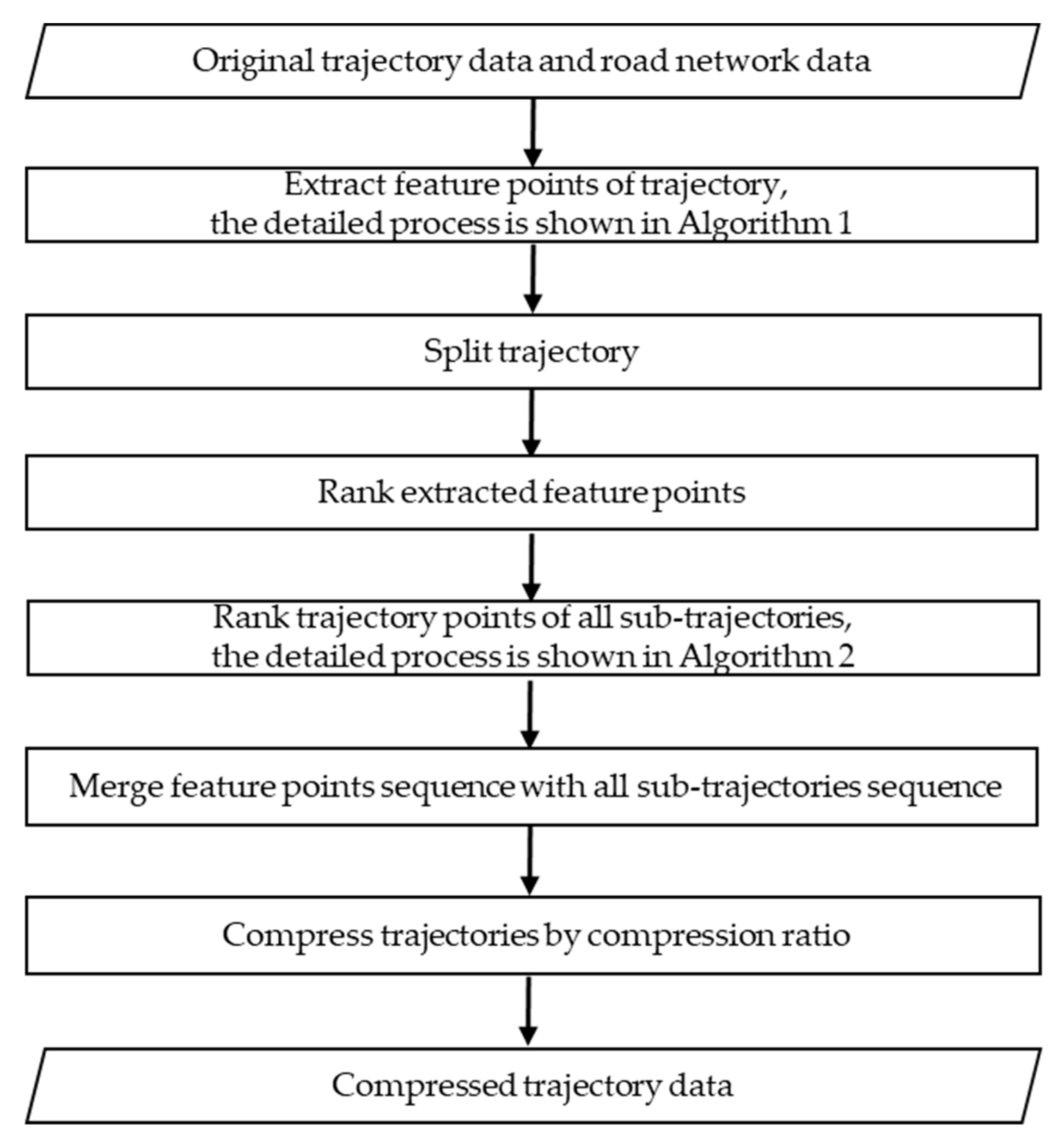
The main idea of this methodology is to rank all trajectory points according to the road network structural characteristics and the spatiotemporal characteristics, then compress the trajectory by deleting the points at the end of the queue in a compression ratio. The workflow chart of this method is shown in Figure 1 and the process is as follows.
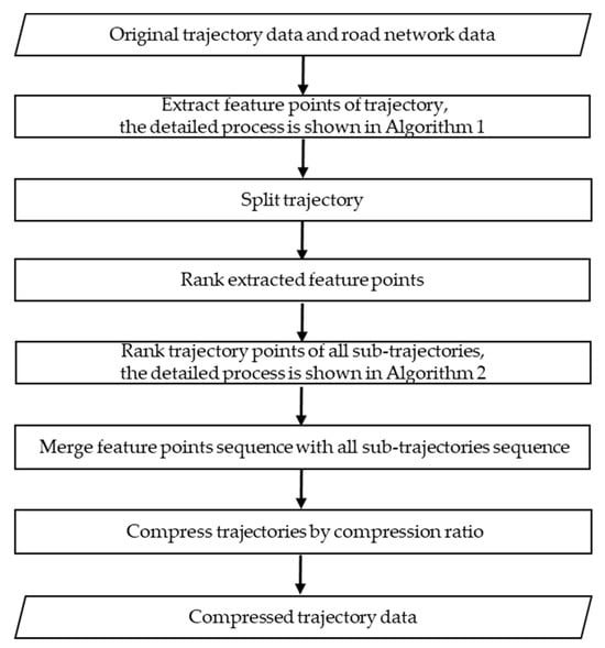
Figure 1.
The workflow chart of this method.
Step 1, to extract feature points in a trajectory with constraints of road networks and split the trajectory at the feature points (Section 2.1);
Step 2, to rank extracted feature points by their feature value (Section 2.2);
Step 3, to rank trajectory points of all sub-trajectories based on the binary line generalization (BLG) tree (Section 2.3);
Step 4, to merge the extracted feature points sequence in step 2 with the trajectory points of every sub-trajectories sequence in step 3, and compress trajectories by removing low-ranking points (Section 2.4).
2.1. Extraction of Trajectory Feature Points
2.1.1. Extraction of Feature Points Based on Road Junctions
The road network in this paper mainly refers to the street network in the city. The main feature of the street network is that there are many intersections, so people or vehicles often stop at the junctions, which leads to multiple trajectory points with similar positions in the trajectory data. Therefore, junctions are always considered as the characteristic points due to their spatial structure. In this research, the feature points in a trajectory are those that are close to the junctions of road networks where the moving object passes by. Here, we take all the closest trajectory points to road junctions as constraint conditions.
Generally, a graph is an ordered pair comprising a set of vertices together with a set of edges. In this paper, the road network is also represented as a modified graph, where represents the set of all nodes in the road network, and is the set of road network edges. In the graph, any edge includes two nodes and a polyline with real spatial co-ordinates connecting these two nodes, , and ; any node includes its spatial co-ordinates and a set of adjacent edges, , where is the subset of E, and it is the set of all edges adjacent to node .
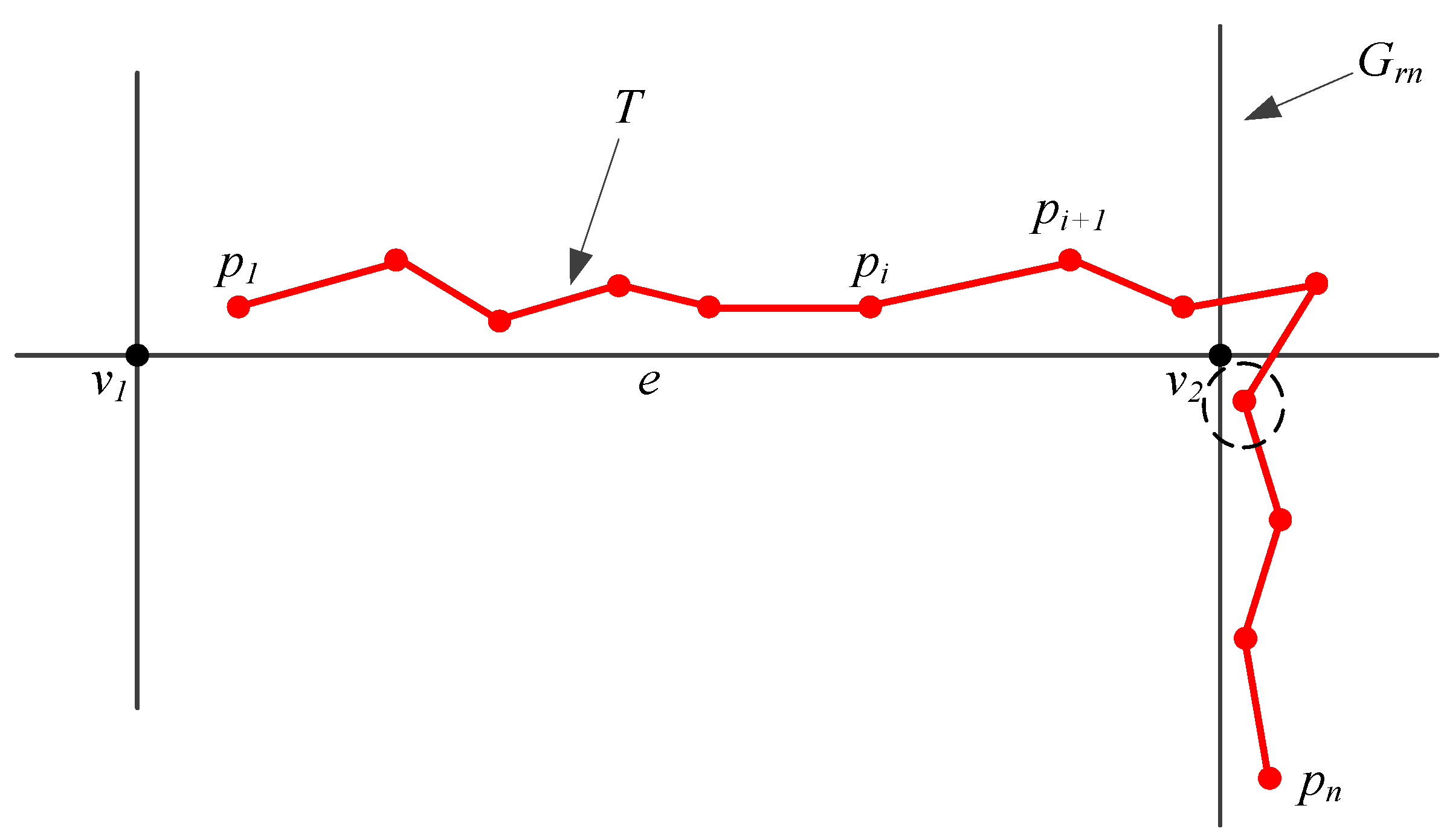
An example of extracting feature points in a trajectory based on road junctions is shown in Figure 2.

Figure 2.
An example of extracting feature points in a trajectory based on road junctions. is a road network graph, where and are junctions, and is an edge. is a schematic trajectory, to are the points of . The point in the dashed circle is the closest to , and it is a feature point of .
In Algorithm 1, a method is proposed to extract the trajectory feature points.
| Algorithm 1. Extraction of feature points based on road junctions |
| Input: A trajectory—T, and road network—(V,E) |
| Output: A list of trajectory feature points—L |
| 1: Set i = 1 |
| 2: Set Et = E//Et is a temporary set of edges |
| 3: While i < n − 1 |
| 4: Find an edge e that is closest to pi |
| 5: Set d1 = dis(pi, e.vl)//dis() is used to obtain the distance between two points |
| 6: Set d2 = dis(pi, e.vr) |
| 7: For j = i + 1 to n |
| 8: Set d1′ = dis(pj, e.vl) |
| 9: Set d2′ = dis(pj, e.vr) |
| 10: IF (d1′ − d1) > 0 and (d2′ − d2) > 0 Then |
| 11: Add pj−1 to L |
| 12: Et = e.vl.Es ∪ e.vr.Es |
| 13: Break For |
| 14: Else IF (d1′ − d1) × (d2′ − d2) < 0 Then |
| 15: d1 = d1′ |
| 16: d2 = d2′ |
| 17: Continue For |
| 18: Else |
| 19: Continue For |
| 20: End IF |
| 21: End For |
| 22: i = j |
| 23: End While |
2.1.2. Trajectory Segmentation at Feature Points
After all feature points are extracted, a trajectory can be divided into several sub-trajectories based on feature points. Due to the design of Algorithm 1, two endpoints are also recognized as feature points. Thus, the count of sub−trajectories is the feature points’ number minus one.
2.2. Trajectory Feature Point Ranking
As shown in Section 2.1, the feature points of the trajectory are extracted based on the junctions in the road network, so their value can be given by their corresponding road junctions. It can be calculated by the road level value associated with the junction as
where is the road level, and is the number of roads connecting to the junction. Roads can be classified as express roads, trunk roads, secondary trunk roads, and branch roads, and their level values are set to 4, 3, 2, and 1, respectively.
2.3. Trajectory Points Ranking of Sub-Trajectories
2.3.1. The BLG Tree Construction
The DP algorithm is the most common method for extracting spatial feature points. It has the anchor point forward method and the divide-and-conquer method, and the latter is usually applied considering the efficiency of the algorithm. The BLG tree [37] is a binary tree structure generated when a curve compression is performed using the divide-and-conquer DP algorithm (threshold is set to 0). Each node in the tree is composed of a point and its eigenvalue. The eigenvalue of a point is the distance from the point to the baseline based on the DP algorithm. In addition, in order to use spatial and temporal characteristics in trajectory compression, this paper constructs a BLG tree based on an improved DP algorithm [2], which fuses temporal characteristics into spatial characteristics by constructing homomorphic Euclidean distance instead of vertical distance.
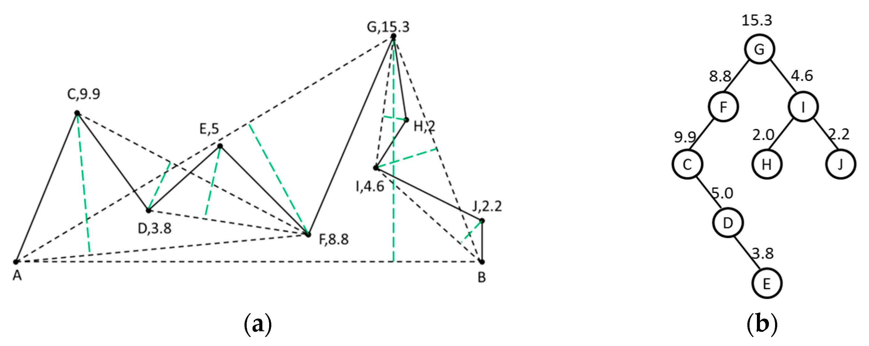
The details of the BLG tree construction are provided by Oosterom [37], and an example of the BLG tree construction is illustrated in Figure 3.

Figure 3.
An example of the BLG tree construction. (a) Process of BLG tree construction. There is a curve example that consists of point sets . Line is the initial baseline. Point is the point with the longest (15.3) distance to the baseline , so it is selected as the root node. Then, points are split into two subsets, and , based on point G. Similarly, points and are points with the longest distance to their baselines, so they are the two child nodes of . By analogy, the tree can be established. (b) Result of this BLG tree construction.
2.3.2. Trajectory Points Ranking
Supposing there are feature points (), the count of sub-trajectories is . For all sub-trajectories, they can be stored in a set , and their BLG trees are . In a tree, a node is represented as node, and its data structure can be illustrated as , where is a trajectory point, is the eigenvalue of a related trajectory point, and and are the left and right child node, respectively. The root node of the tree can be represented as . A ranking method of trajectory points based on the BLG tree for all sub-trajectories is given by Algorithm 2.
| Algorithm 2. Trajectory points ranking for all sub-trajectories based on the BLG tree |
| Input: A set of BLG trees—{Treej|0 ≤ j ≤ m − 1} |
| Output: A queue arranged by descending order of importance—Q |
| 1: Set Q as an empty queue |
| 2: Set S as a candidate set to store nodes temporarily |
| 3: For j = 1 to m − 1 |
| 4: Put root node rootj of Treej into S |
| 5: Next j |
| 6: While S is not empty |
| 7: Find the node nodemax with maximum eigenvalue (ev) inside the S |
| 8: Put nodemax into Q |
| 9: Put nodemax.lcn, nodemax.rcn into S |
| 10: Remove nodemax from S |
| 11: End While |
As a BLG tree does not contain the endpoints of a sub-trajectory, the outputted queue of trajectory points also avoids all feature points tactfully.
An example of trajectory points ranking based on the BLG tree is shown in Figure 4 and Table 1. In the Figure 4, is the root of the tree, and it is added into set first. There is only one node in , so the node is selected to put into and removed from in the first step. In the second step, the children , of is put into , and F has a maximum eigenvalue. Thus, is added to and removed from set . Following the algorithm, the output result of queue is .
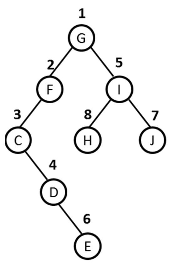
Figure 4.
An example of a BLG tree.

Table 1.
The process of trajectory points ranking based on the BLG tree in Figure 4.
2.4. All Trajectory Points Ranking and Compression
The trajectory feature points always have higher importance than other points, so the whole trajectory ranking is composed of ranked feature points first, which are obtained from Step 2, and the other ranked sub-trajectory points from Step 3.
After obtaining the queuing results of trajectory points, it is possible to quickly obtain compression results at any compression ratios according to removing the corresponding proportion of points from the tail of the queue.
3. Experiments and Results
3.1. Experimental Setup
The experimental data comprise road network data and trajectory data. The road network data are all levels of roads in Beijing’s urban area. The trajectory data comprise two taxis’ trajectory datasets during the period of 2–8 February 2008 within Beijing [38]. They are shown in Figure 5, and the details of trajectory data are listed in Table 2.
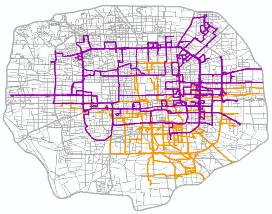
Figure 5.
Experimental data. Color lines are trajectory data, whereas the purple lines are dataset 1 and the orange lines are dataset 2. Gray lines are the road network data, and the width of the line represents the road level.
Table 2.
Information about the data of the two trajectories.
For the applicability of the experiment, two trajectories with different sampling frequencies were selected. As shown in Table 1, the sampling interval of dataset 1 is 5 s, the number of points is 30,156, and the length is 1,098,329 m; the sampling interval of dataset 2 is 15 s, the number of points is 7141, and the length is 853,270 m.
The method was implemented in C#.NET with ArcGIS plugins for the trajectory and map data importing and visualization. In this experiment, the proposed TSRC method is applied to test the experiment data, and results are discussed by comparing the TSRC method with the TD–TR (top-down time ratio) method proposed by Meratnia and Rolf [2]. Because the TD−TR method is a compression method by threshold value, it is difficult to obtain the compression result of a given compression ratio directly. In order to compare the proposed method with the TD−TR method under the same compression ratio, the damping oscillation method proposed in paper [39] is adopted. In this method, a given compression ratio is obtained by adjusting the threshold value in the TD−TR method. In addition, in order to perform comparative analysis on various compression ratios, nine compression ratios of 0.1, 0.2, 0.3, 0.4, 0.5, 0.6, 0.7, 0.8 and 0.9 were used in the experiment.
The comparative analysis experiment consists of two parts. First, the visualization, accuracy, and efficiency of compression are discussed by comparing the TSRC method and the TD–TR method. Second, these two methods are each combined with map matching, and the accuracy and efficiency of their compression are compared.
3.2. Accuracy Assessment Method
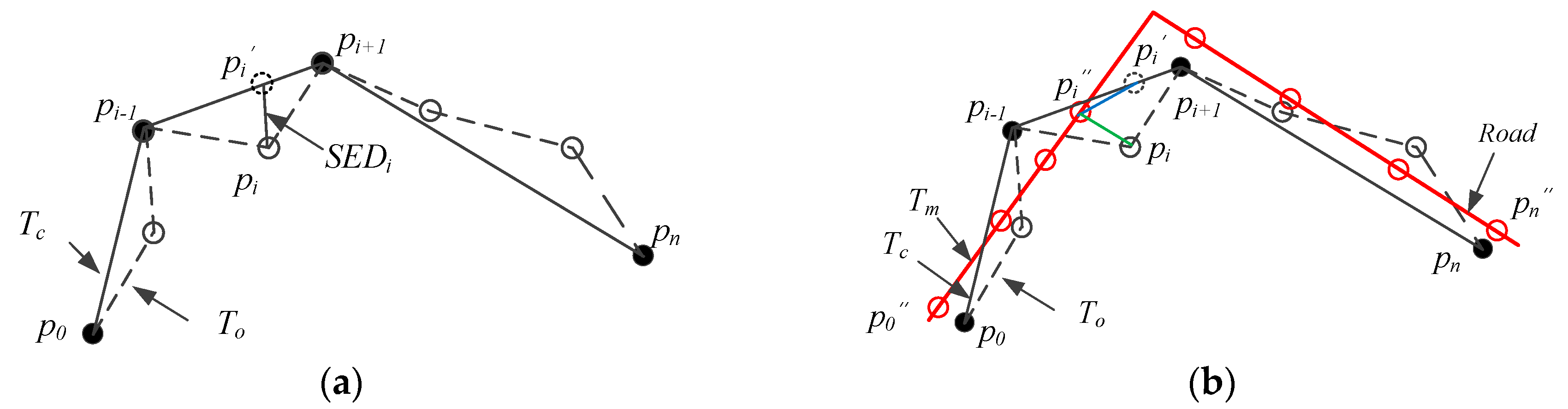
For the accuracy metrics, a synchronized Euclidean distance (SED) error is used to perform the validation [2]. The SED is the distance between the original trajectory point and its compressed trajectory point , which is the synchronized point of in the compressed trajectory. Figure 6a illustrates a schematic of SED.
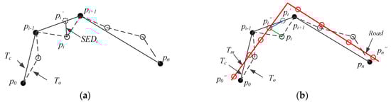
Figure 6.
Schematics of SED and NSED errors. (black dashed line), (solid black line), and (red line) are original, compressed, and matched trajectories, respectively, is the synchronized point of in , and is the matched point of in . (a) SED error: is the distance between and . (b) Proposed NSED error: is the matching error of the original trajectory point (the distance between and ) minus the matching error of the original trajectory point (the distance between and ).
However, the trajectory usually matches the road network, so an error of a removed point should be compared to the distance to the road, not to the compressed trajectory. Therefore, this research proposes an improved error assessment method based on SED error, the so-called network-based synchronized Euclidean distance (NSED) error. It uses the matched trajectory as the reference data instead of the original trajectory. After that, the NSED error is calculated as the difference between the matching error of the compressed trajectory and the original trajectory. A schematic of NSED can be seen in Figure 6b.
In the experiment, the average NSED errors are adopted to evaluate the accuracy between an original trajectory and its compressed trajectory, and it can be given as follows:
where a is the average NSED errors, is the original trajectory point, is the synchronized point of , is the matched point of , and is the distance between two points.
3.3. Results
3.3.1. Visual Assessment Results
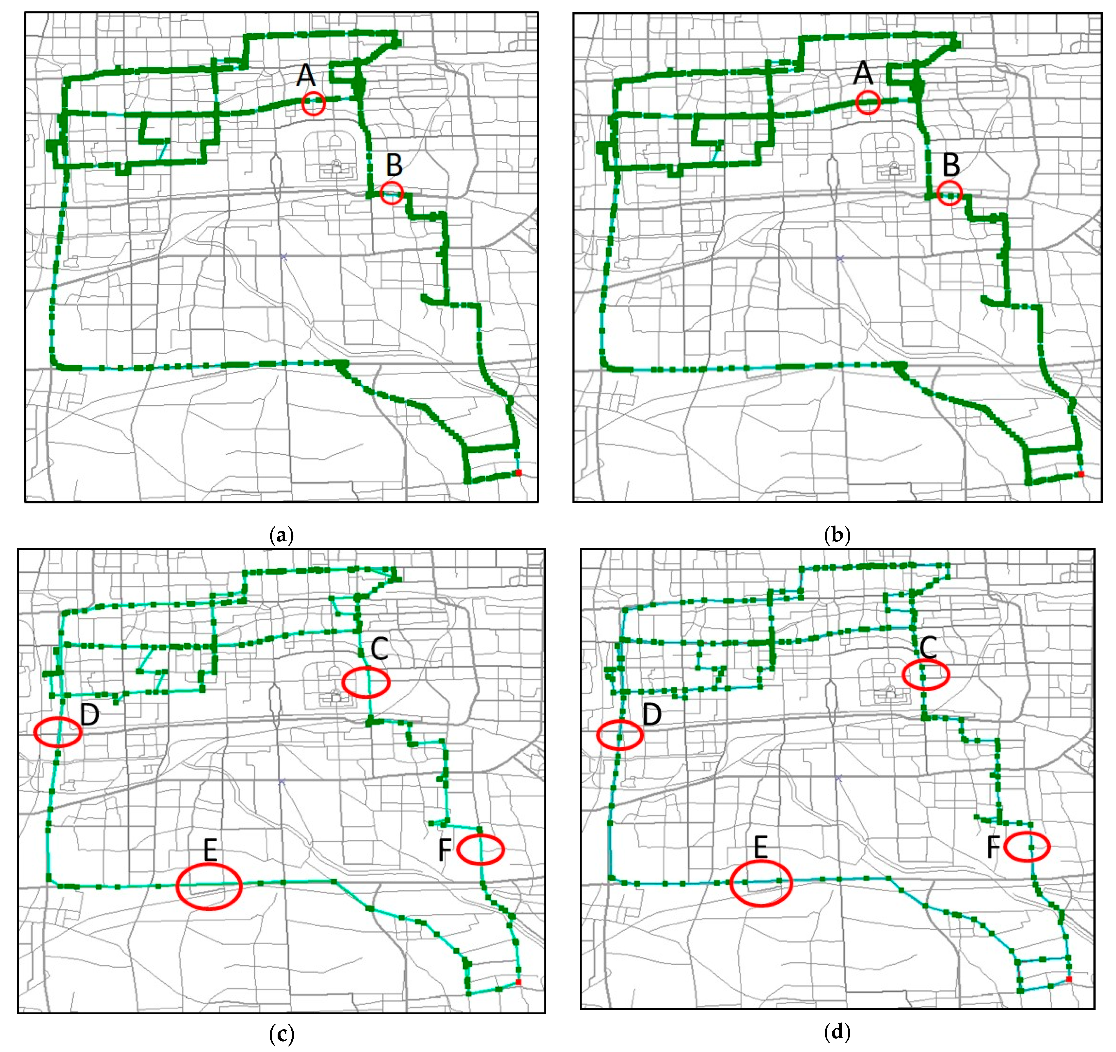
The visual assessment is designed to compare the remaining trajectory feature points between the TSRC method and the TD–TR method. As shown in Figure 7, first, both methods retain the trajectory points with prominent spatial characteristics. Second, comparing (a), (c) to (b), (d) in red circles, the TSRC method also retains the trajectory points close to the road network nodes. In addition, when the compression rate increases, the TSRC method can better retain the trajectory points close to the road network nodes than the TD-TR method. For example, the feature points in red circles C, D, E, and F are removed in Figure 7c but reserved in Figure 7d. In general, the TSRC method can better retain the trajectory points with prominent spatial characteristics and the road network structure characteristics, while the TD–TR method can only retain the trajectory points with spatial characteristics.
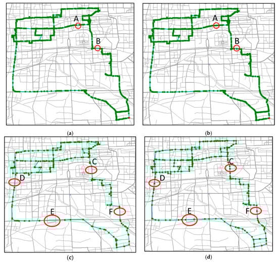
Figure 7.
Visual assessment results between the TSRC method and the TD–TR method in partial dataset 1. The green lines are the simplified trajectory lines, and the red circles are the positions where trajectory feature points remain inconsistent between the two compression methods. (a,b) are the results of TD–TR method and TSRC method respectively with compression ratio 50%; (c,d) are the results of TD–TR method and TSRC method respectively with compression ratio 90%.
3.3.2. Efficiency Assessment Results
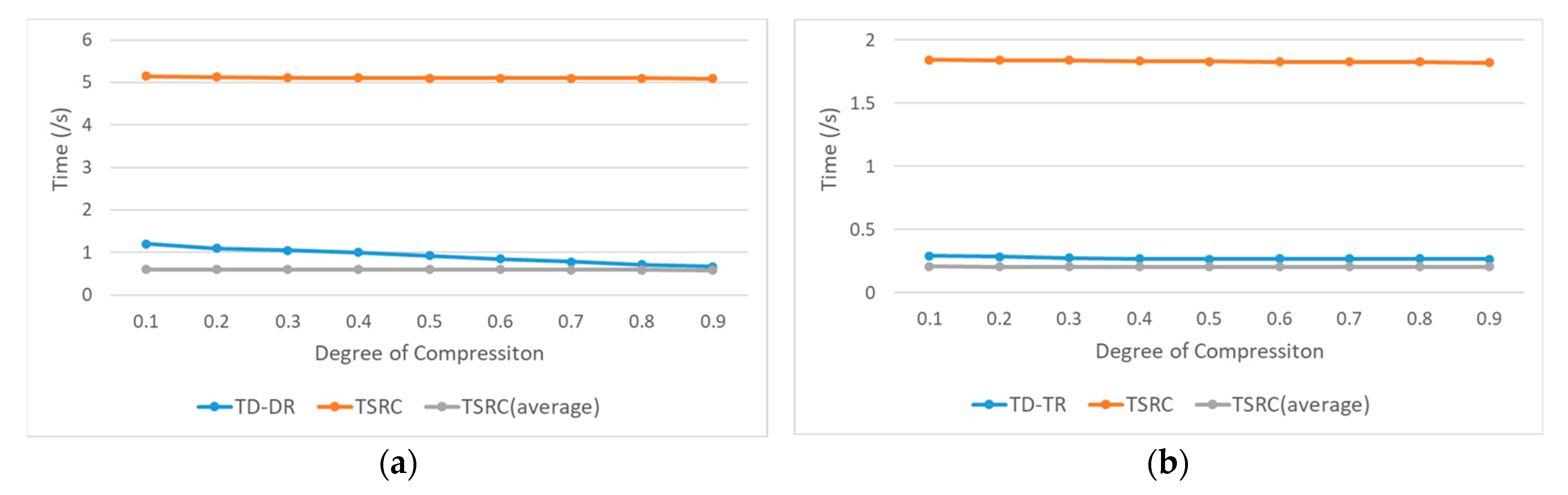
The efficiency between the TSRC method and the TD–TR method was compared at nine compression ratios from 0.1 to 0.9. Since the TSRC method only needs to be queued once, the results of any different compression ratios can be obtained. Therefore, the efficiency of the TSRC method is evaluated by the independent efficiency and average efficiency. The efficiency assessment results are shown in Figure 8.
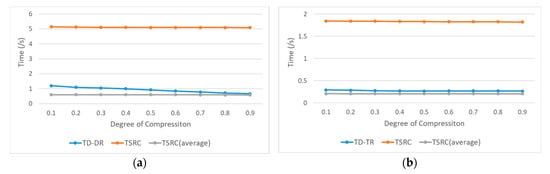
Figure 8.
Efficiency comparison between the TD–TR method and the TSRC method at nine thresholds. The blue lines are the running time of the TD–TR method. The orange lines are the running time of the TSRC method for independent efficiency. The gray lines are the running time of the TSRC method for average efficiency. (a,b) are the result of dataset 1 and dataset 2, respectively.
As shown in Figure 8a,b, in the two experimental datasets, the running time of the TSRC method is greater than the TD–TR method. Moreover, the running time of the TSRC method does not change with the increase in compression ratio, while the running time of the TD–TR method decreases slightly with the increase in compression ratio.
However, considering multiple compression ratios, the average running time of the TSRC method is lower than the TD–TR method. Moreover, the more compression ratios, the higher the average efficiency of TSRC. For example, there are nine compression ratios in the above experiment, so the average efficiency of the TSRC method can be improved by nine times. Therefore, the TSRC method is more suitable for data compression with multiple compression ratios.
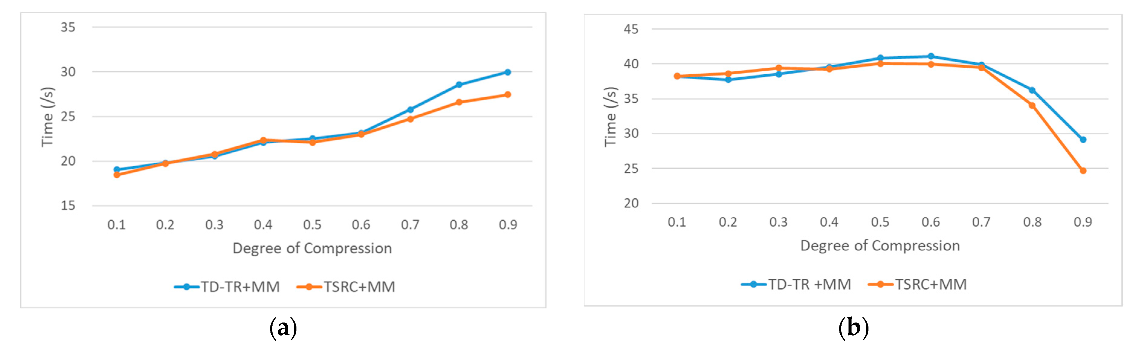
Considering that trajectory data often require map matching, the trajectory is compressed by the TSRC method and the TD–TR method and then matched to roads. The matching method uses the “look−ahead” method [21]. Thus, the following experiments compare the overall efficiency of trajectory compression and map matching, as shown in Figure 9.
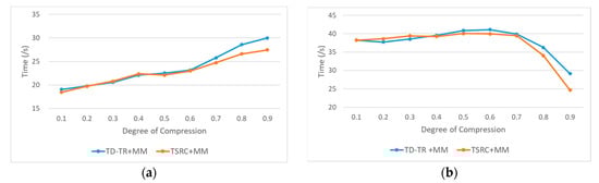
Figure 9.
Efficiency comparison of the TSRC method and the TD–TR method combined with the map matching (MM) method. Here, TD–TR+MM and TSRC + MM are abbreviations. (a,b) are the result of dataset 1 and dataset 2, respectively.
Figure 9 shows that the running times of the TSRC + MM and TD−TR + MM methods are much longer than those of the TSRC and TD−TR methods in Figure 8, as the map matching process takes a long time. With the increase in compression ratio, the changing trend of the running time of the TSRC + MM method is consistent with the TD−TR + MM method, but the TSRC + MM method is more efficient than the TD−TR + MM method. It shows that the TSRC method will improve the efficiency of map matching, and its efficiency can be improved more significantly as the compression ratio becomes larger. This is because the TSRC method can retain trajectory points close to the road network nodes, thereby avoiding missing track points on a specific road section, and finally improving the search efficiency of the road network during map matching.
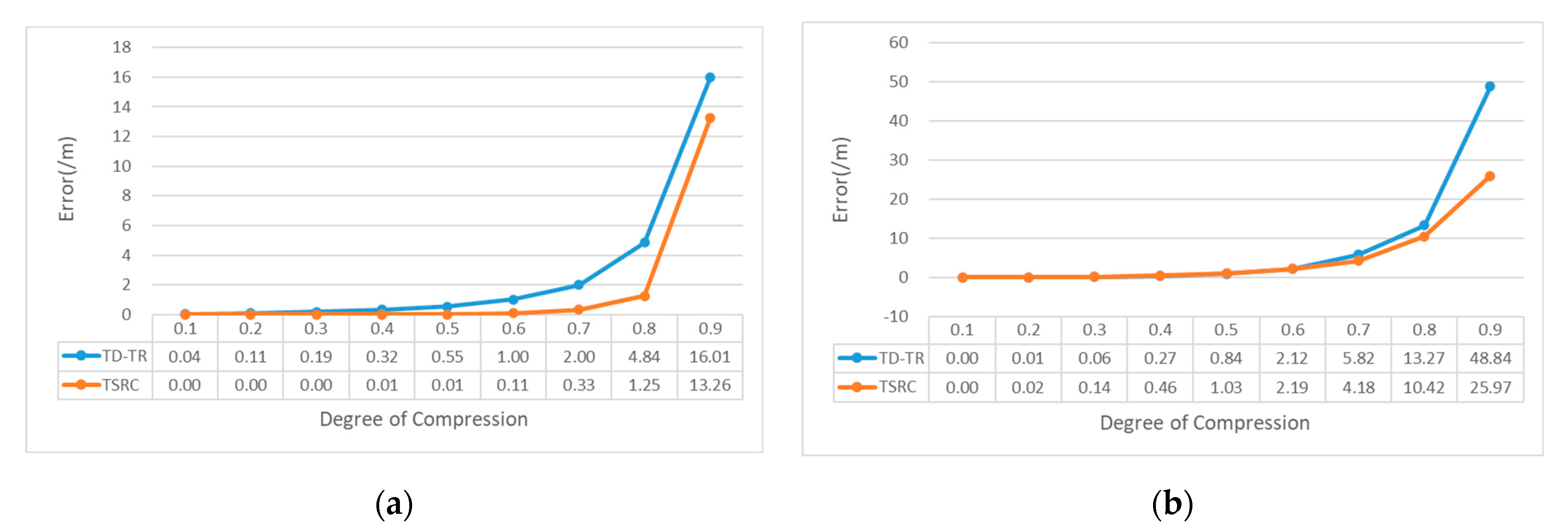
3.3.3. Accuracy Assessment Results
The accuracy assessment method uses the network-based synchronized Euclidean distance NSED error mentioned in Section 3.2. In order to eliminate the error of the original data, the accuracy result is that the NSED error of the compressed trajectory is subtracted from the NSED error of the original trajectory. Similarly, the accuracy between the TSRC method and TD−TR method was compared for nine compression ratios from 0.1 to 0.9. The accuracy assessment results are shown in Figure 10.
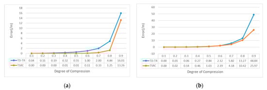
Figure 10.
Accuracy comparison between the TSRC method and the TD−TR method at nine thresholds. The blue lines are the error of the TD−TR method. The orange lines are the error of the TSRC method. (a,b) are the result of dataset 1 and dataset 2, respectively.
The following is shown in Figure 10: (1) The error of the two methods becomes large gradually with the increase in compression ratio, and when the compression ratio is greater than 0.5, the error increases significantly. (2) The error of the TSRC method is smaller than that of the TD–TR method. (3) The error difference between the two methods becomes large with the increase in compression ratio. The gap is evident at a compression rate of 0.5 in dataset 1 and a rate of 0.7 in dataset 2.
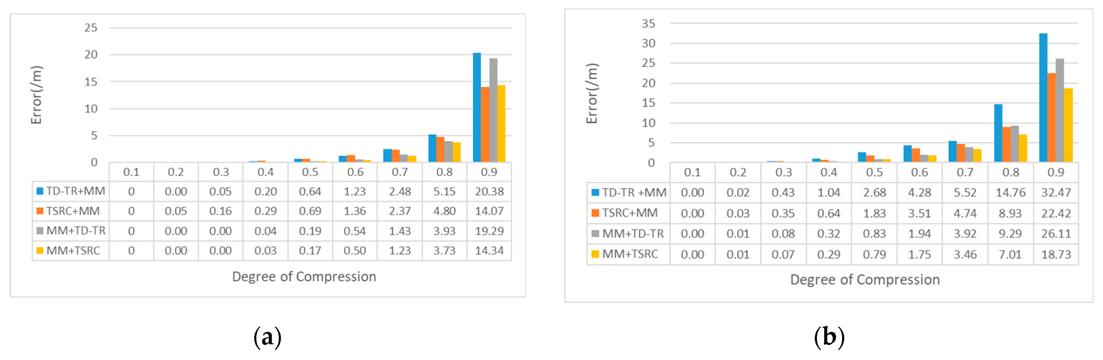
Considering that the trajectory after map matching is close to the real data, the following four mixed methods are compared: TSRC compression before map matching (TSRC + MM), TD–TR compression before map matching (TD–TR + MM), map matching before TSRC compression (MM + TSRC), and map matching before TD–TR compression (MM + TD–TR). Since the trajectory data have been map-matched, the accuracy assessment method uses an SED error instead. The results are shown in Figure 11.
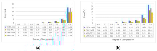
Figure 11.
Accuracy comparison of the TSRC method and the TD–TR method combined with the map-matching algorithm. (a,b) are the result of dataset 1 and dataset 2, respectively.
From Figure 11, we find the following: (1) In general, the accuracy order of the four combination methods is MM + TSRC > MM + TD-TR > TSRC + MM > TD–TR + MM. Thus, the accuracy of the trajectory compression after map matching is greater than that of map matching after trajectory compression. (2) In trajectory compression after map matching, the accuracy of the MM + TSRC method is higher than that of the MM+TD–TR method. (3) In map matching after trajectory compression, when the compression ratio is small (such as when the dataset 1 compression ratio is less than 0.6 and the dataset 2 compression ratio is less than 0.2), the TSRC + MM method has lower accuracy than the TD–TR + MM one. When the ratio becomes more significant, the accuracy of the TSRC + MM is higher.
4. Conclusions
Based on spatiotemporal characteristics and road network structure characteristics, this paper proposes the trajectory segmentation and ranking compression (TSRC) method based on a road network and designs the network homomorphic distance error for accuracy evaluation. Based on a comparison with the TD–TR method, the following conclusions can be drawn.
First, the proposed TSRC algorithm can retain not only trajectory points with significant spatiotemporal characteristics but also trajectory points with significant road network structural characteristics.
Second, although the TSRC method is less efficient than the TD–TR method, the TSRC method can improve the efficiency of map matching after compression. This is because it retains more trajectory points with significant road network structural characteristics. In addition, the efficiency of the TSRC method is affected by the number of compression ratios and the amount of road network data, as it queues once and compresses multiple times. The more compression ratios required, the more efficient the TSRC method is. Moreover, the number of road network data will affect the efficiency of the feature-point extraction in the TSRC method.
Third, the TSRC method has higher accuracy with the assessment of the NSED error. As the compression ratio increases, the gap between the TSRC method and the TD–TR method gradually increases. Moreover, when the combination of the trajectory compression method and map-matching method is analyzed, the accuracy of the TSRC combination method is higher than that of the TD–TR combination method. In addition, the accuracy of map matching before trajectory compression is higher than that of map matching after trajectory compression. This result is evident because map matching after trajectory compression produces more matching errors.
Author Contributions
Conceptualization, Minshi Liu; methodology, Minshi Liu and Yong Sun; formal analysis, Minshi Liu and Ling Zhang; writing—original draft preparation, Minshi Liu; writing—review and editing, Ling Zhang and Yi Long; visualization, Mingwei Zhao; supervision, Ling Zhang and Yi Long; funding acquisition, Ling Zhang and Minshi Liu. All authors have read and agreed to the published version of the manuscript.
Funding
This research was funded by the National Natural Science Foundation of China, grant number 41601499, the Key/Major of University Natural Science Research Project of Anhui Province, grant number 2022AH051113, 2022AH040150, the Guiding Plan Project of Chuzhou Science and Technology Bureau, grant number 2021ZD008, and the Foundation of Anhui Province Key Laboratory of Physical Geographic Environment, grant number 2022PGE003.
Data Availability Statement
The data that support the findings of this study are openly available in figshare at https://figshare.com/s/c9c521c86a1a8ee3f84d (accessed on 6 October 2023).
Acknowledgments
The authors would like to thank Microsoft Research Asia for providing T-Drive data support.
Conflicts of Interest
The authors declare no conflict of interest. The funders had no role in the design of the study; in the collection, analyses, or interpretation of data; in the writing of the manuscript, and in the decision to publish the results.
References
- Deng, M.; Huang, J.C.; Zhang, Y.F.; Liu, H.M.; Tang, L.L.; Tang, J.B.; Yang, X.X. Generating Urban Road Intersection Models from Low-frequency GPS Trajectory Data. Int. J. Geogr. Inf. Sci. 2018, 32, 2337–2361. [Google Scholar] [CrossRef]
- Huang, J.C.; Tang, J.B. Discovery of arbitrarily shaped significant clusters in spatial point data with noise. Appl. Soft Comput. 2021, 108, 107452. [Google Scholar] [CrossRef]
- Meratnia, N.; de By, R.A. Spatiotemporal Compression Techniques for Moving Point Objects. In Proceedings of the Advances in Database Technology—EDBT 2004, Crete, Greece, 14–18 March 2004; Springer: Berlin/Heidelberg, Germany, 2004; pp. 765–782. [Google Scholar] [CrossRef]
- Cao, H.; Wolfson, O.; Trajcevski, G. Spatio-temporal data reduction with deterministic error bounds. VLDB J. 2006, 15, 211–228. [Google Scholar] [CrossRef]
- Muckell, J.; Olsen, P.W.; Hwang, J.-H.; Lawson, C.T.; Ravi, S.S. Compression of trajectory data: A comprehensive evaluation and new approach. Geoinformatica 2014, 18, 435–460. [Google Scholar] [CrossRef]
- Douglas, D.H.; Peucker, T.K. Algorithms for the reduction of the number of points required to represent a digitized line or its caricature. Cartogr. Int. J. Geogr. Inf. Geovis. 1973, 10, 112–122. [Google Scholar] [CrossRef]
- Yin, H.; Gao, H.; Wang, B.; Li, S.; Li, J. Efficient trajectory compression and range query processing. World Wide Web 2022, 25, 1259–1285. [Google Scholar] [CrossRef]
- Zhong, Y.; Kong, J.; Zhang, J.; Jiang, Y.; Fan, X. A trajectory data compression algorithm based on spatio-temporal characteristics. PeerJ Comput. Sci. 2022, 8, e1112. [Google Scholar] [CrossRef] [PubMed]
- Fikioris, G.; Patroumpas, K.; Artikis, A.; Pitsikalis, M.; Paliouras, G. Optimizing vessel trajectory compression for maritime situational awareness. GeoInformatica 2022, 27, 565–591. [Google Scholar] [CrossRef]
- Zhao, L.; Shi, G. A method for simplifying ship trajectory based on improved Douglas–Peucker algorithm. Ocean. Eng. 2018, 166, 37–46. [Google Scholar] [CrossRef]
- Zhao, Y.; Shang, S.; Wang, Y.; Zheng, B.L.; Nguyen, Q.V.H.; Zheng, K. Rest: A reference-based framework for spatio-temporal trajectory compression. In Proceedings of the 24th ACM SIGKDD International Conference on Knowledge Discovery & Data Mining, London, UK, 19–23 August 2018. [Google Scholar] [CrossRef]
- Liu, J.; Zhao, K.; Sommer, P.; Shang, S.; Kusy, B.; Lee, J.G.; Jurdak, R. A novel framework for online amnesic trajectory compression in resource-constrained environments. IEEE Trans. Knowl. Data Eng. 2016, 28, 2827–2841. [Google Scholar] [CrossRef]
- Deng, Z.; Han, W.; Wang, L.; Ranjan, R.; Zomaya, A.Y.; Jie, W. An efficient online direction-preserving compression approach for trajectory streaming data. Future Gener. Comput. Syst. 2017, 68, 150–162. [Google Scholar] [CrossRef]
- Tao, J.C.; Chen, L.; Fang, J.H. A novel real-time trajectory compression method for privacy protection. In Proceedings of the 2022 IEEE 9th International Conference on Data Science and Advanced Analytics (DSAA), Online, 13–16 October 2022. [Google Scholar] [CrossRef]
- Fazzinga, B.; Flesca, S.; Masciari, E.; Furfaro, F. Efficient and effective RFID data warehousing. In Proceedings of the 2009 International Database Engineering & Applications Symposium, Cetraro, Italy, 16–18 September 2009. [Google Scholar] [CrossRef]
- Fazzinga, B.; Flesca, S.; Furfaro, F. RFID-data compression for supporting aggregate queries. ACM Trans. Database Syst. (TODS) 2013, 38, 1–45. [Google Scholar] [CrossRef]
- Makris, A.; Kontopoulos, I.; Alimisis, P.; Tserpes, K. A comparison of trajectory compression algorithms over AIS data. IEEE Access 2021, 9, 92516–92530. [Google Scholar] [CrossRef]
- Tang, C.H.; Wang, H.; Zhao, J.H.; Tang, Y.Q.; Yan, H.R. A method for compressing AIS trajectory data based on the adaptive-threshold Douglas-Peucker algorithm. Ocean Eng. 2021, 232, 109041. [Google Scholar] [CrossRef]
- Kellaris, G.; Pelekis, N.; Theodoridis, Y. Map-matched trajectory compression. J. Syst. Softw. 2013, 86, 1566–1579. [Google Scholar] [CrossRef]
- Ta, N.; Li, G.L.; Chen, B.; Feng, J.H. Semantic-aware trajectory compression with urban road network. In Lecture Notes in Computer Science; Cui, B., Zhang, N., Xu, J., Lian, X., Liu, D., Eds.; Springer: Cham, Switzerland, 2016; pp. 124–136. [Google Scholar] [CrossRef]
- Liu, K.; Li, Y.; Dai, J.; Shang, S.; Zheng, K. Compressing large scale urban trajectory data. In Proceedings of the Fourth International Workshop on Cloud Data and Platforms—CloudDP ’14, Amsterdam, The Netherlands, 13 April 2014; Association for Computing Machinery: New York, NY, USA, 2014. [Google Scholar] [CrossRef]
- Li, T.Y.; Chen, L.; Jensen, C.S.; Pedersen, T.B. TRACE: Real-time compression of streaming trajectories in road networks. Proc. VLDB Endow. 2021, 14, 1175–1187. [Google Scholar] [CrossRef]
- Song, R.; Sun, W.; Zheng, B.; Zheng, Y. PRESS: A novel framework of trajectory compression in road networks. Comput. Sci. 2014, 7, 661–672. [Google Scholar] [CrossRef]
- Sandu Popa, I.; Zeitouni, K.; Oria, V.; Kharrat, A. Spatio-temporal compression of trajectories in road networks. Geoinformatica 2015, 19, 117–145. [Google Scholar] [CrossRef]
- Hsueh, Y.L.; Chen, H.C. Map matching for low-sampling-rate GPS trajectories by exploring real-time moving directions. Inf. Sci. 2018, 433, 55–69. [Google Scholar] [CrossRef]
- Liu, M.S.; Zhang, L.; Ge, J.L.; Long, Y. Map matching for urban high-sampling-frequency GPS trajectories. ISPRS Int. J. Geo-Inf. 2020, 9, 31. [Google Scholar] [CrossRef]
- Knapen, L.; Bellemans, T.; Janssens, D.; Wets, G. Likelihood-based offline map matching of GPS recordings using global trace information. Transp. Res. Part C Emerg. Technol. 2018, 93, 13–35. [Google Scholar] [CrossRef]
- Yang, C.; Gidofalvi, G. Fast map matching, an algorithm integrating hidden Markov model with precomputation. Int. J. Geogr. Inf. Sci. 2018, 32, 547–570. [Google Scholar] [CrossRef]
- Zhu, L.; Holden, J.R.; Gonder, J.D. Trajectory Segmentation Map-Matching Approach for Large-Scale, High-Resolution GPS Data. Transp. Res. Rec. 2017, 2645, 67–75. [Google Scholar] [CrossRef]
- Richter, K.-F.; Schmid, F.; Laube, P. Semantic trajectory compression: Representing urban movement in a nutshell. J. Spat. Inf. Sci. 2012, 4, 3–30. [Google Scholar] [CrossRef]
- Feng, S.; Xu, J.; Xu, M.; Zheng, N.; Zhang, X. EHSTC: An enhanced method for semantic trajectory compression. In Proceedings of the 4th ACM SIGSPATIAL International Workshop on GeoStreaming—IWGS ’13, Orlando, FL, USA, 5 November 2013; ACM Press: New York, NY, USA, 2013; pp. 43–49. [Google Scholar] [CrossRef]
- Han, Y.H.; Sun, W.W.; Zheng, B.H. COMPRESS: A comprehensive framework of trajectory compression in road networks. ACM Trans. Database Syst. (TODS) 2017, 42, 11. [Google Scholar] [CrossRef]
- Liu, S.; Chen, G.; Wei, L.; Li, G. A novel compression approach for truck GPS trajectory data. IET Intell. Transp. Syst. 2021, 15, 74–83. [Google Scholar] [CrossRef]
- Iiyama, S.; Oda, T.; Hirota, M. An algorithm for GPS trajectory compression preserving stay points. In Lecture Notes on Data Engineering and Communications Technologies; Barolli, L., Kulla, E., Ikeda, M., Eds.; Springer: Cham, Switzerland, 2022; pp. 102–113. [Google Scholar] [CrossRef]
- Zhu, F.; Ma, Z. Ship Trajectory Online Compression Algorithm Considering Handling Patterns. IEEE Access 2021, 9, 70182–70191. [Google Scholar] [CrossRef]
- Zhang, K.; Zhao, D.; Liu, W. Online vehicle trajectory compression algorithm based on motion pattern recognition. IET Intell. Transp. Syst. 2022, 16, 998–1010. [Google Scholar] [CrossRef]
- Oosterom, P.V. The reactive-tree: A storage structure for a seamless, scaleless geographic database. In Proceedings of the Tenth International Symposium on Computer-Assisted Cartography, AUTO-CARTO 10, Baltimore, MD, USA, 25–28 March 1991; ACSM/ASPRS: Baltimore, MD, USA, 1991; pp. 393–407. [Google Scholar]
- Yuan, J.; Zheng, Y.; Xie, X.; Sun, G. Driving with knowledge from the physical world. In Proceedings of the 17th ACM Sigkdd International Conference on Knowledge Discovery and Data Mining, New York, NY, USA, 21–24 August 2011; pp. 316–324. [Google Scholar] [CrossRef]
- Liu, M.; Long, Y.; Fei, L. Line simplification of three-dimensional drainage considering topological consistency. Acta Geod. Et Cartogr. Sin. 2016, 45, 494–501. [Google Scholar] [CrossRef]


Disclaimer/Publisher’s Note: The statements, opinions and data contained in all publications are solely those of the individual author(s) and contributor(s) and not of MDPI and/or the editor(s). MDPI and/or the editor(s) disclaim responsibility for any injury to people or property resulting from any ideas, methods, instructions or products referred to in the content. |
© 2023 by the authors. Licensee MDPI, Basel, Switzerland. This article is an open access article distributed under the terms and conditions of the Creative Commons Attribution (CC BY) license (https://creativecommons.org/licenses/by/4.0/).