

Areas of Crime in Cities: Case Study of Lithuania

Abstract
:1. Introduction
- (a)
- Detailed inventory maps providing precise (address/point-level) information on events (Figure 1a). This is usually sensitive data, as known facts about some types of events may reduce the value of the property or, in sparsely populated areas, even be linked to individual persons, thus violating their right to privacy.
- (b)
- Generalised inventory maps, which provide data on the density and/or frequency of events at a spatial resolution that does not allow the identification of a precise location or person (Figure 1b). The aggregation can be performed in various ways, such as based on statistical grids, administrative units or clusters or by creating a statistical density surface (in this case, the data are further interpolated between points, thus creating certain distortions).
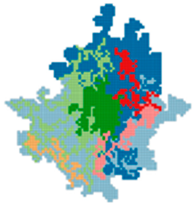
- (c)
- Analytical maps, where derived characteristics such as density, hotspots, etc., are presented. Analytical maps help to identify patterns and trends (Figure 1c). In such maps, crime data are often linked to indicators that may influence the distribution of crime.
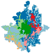
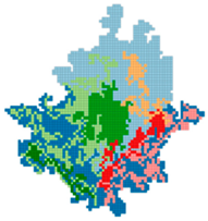
- (d)
- Regionalisation maps, which divide the territory into a relatively small number of contiguous areas that differ in terms of certain characteristics, i.e., so-called regions or areas of crime (Figure 1d).
- Which of the known spatial clustering methods achieves the best validity for given country-specific crime data?;
- Is it possible to identify districts that are consistent with a common understanding of the characteristics of urban areas?
- (a)
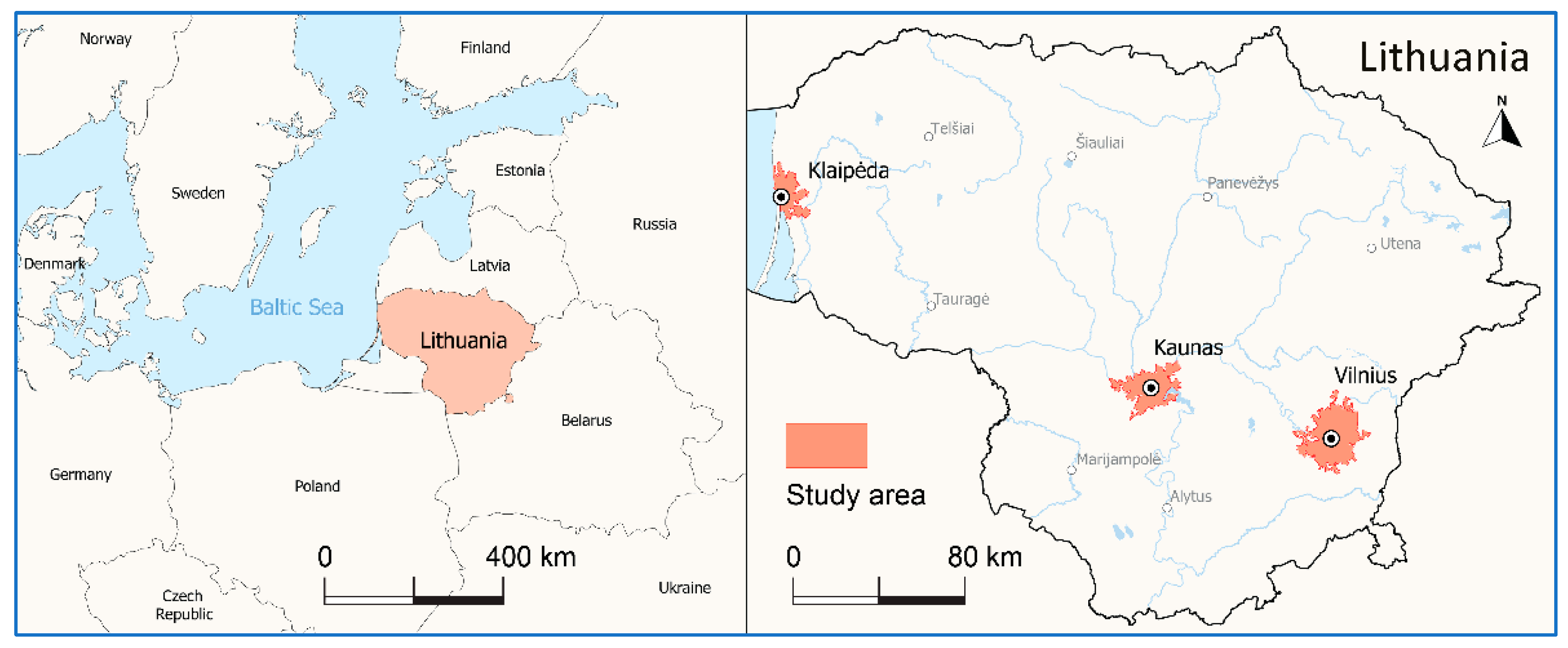
- The regionalisation is carried out in cities rather than in large areas. It is a pilot study with the aim of contributing to better crime management in densely populated areas.
- (b)
- The variables of the regionalisation are primarily related to the structure of crime, distinguishing between open spaces and private/semi-private spaces.
- (c)
- Aggregated data divided into five classes are used for regionalisation. This reduces distortions due to very small or occasionally very large values.
2. Previous Research
3. Materials and Methods
3.1. Experiment Design
- Systematising insights from the literature and previous regionalisation experiments.
- Preparing data for analysis:
- Geocoding and cleaning of RERP crime data;
- The aggregation of point-event data in a grid of 500 m × 500 m cells that were further used as inputs for spatial clustering;
- Adding summarised population data;
- The reclassification of event count values;
- The identification of urban and suburban areas to be investigated.
- Experimental selection of a regionalisation method:
- The selection of the initial number of clusters;
- The application and evaluation of different spatial clustering methods for each city;
- Experiments changing the number of clusters via the selected methods;
- The selection of the most suitable clustering method and the number of clusters.
- Regionalisation and mapping.
- Analysis and interpretation of the outcomes.
3.2. Data
- Violent crime (VIO), such as homicide, murder, assault, manslaughter (bodily injury), sexual assault, rape, robbery, abduction and harassment;
- Property offences (PRO), such as theft, destruction or damage to property;
- The infringement of public policy (IPP), such as breaches of the peace, illicit consumption of alcohol, noise, littering, etc.
3.3. Selection of Spatial Clustering Method
- AZP: the automatic zoning procedure (AZP) uses heuristics to find the best set of combinations of contiguous spatial units into p regions, minimizing the within sum of squares as a criterion of homogeneity.
- SCHC: Spatially constrained hierarchical clustering algorithm. This method builds up the clusters using the following agglomerative hierarchical clustering methods: single linkage, complete linkage, average linkage and Ward’s linkage (a special form of centroid linkage).
- SKATER: the divisive hierarchical clustering algorithm based on the optimal pruning of a minimum spanning tree into several clusters, seeking the maximal similarity of the values of the selected variables while retaining spatial contiguity.
- REDCAP: Regionalisation with dynamically constrained agglomerative clustering and partitioning. It builds a spanning tree in 4 different ways (single linkage, average linkage, Ward’s linkage and complete linkage). It also provides 2 different ways (first-order and full-order constraining) of pruning the tree to find clusters.
4. Results
5. Discussion and Conclusions
Author Contributions
Funding
Data Availability Statement
Acknowledgments
Conflicts of Interest
References
- Colaninno, N. Insights into Heat islands at a Regional Scale using a Data-driven Approach. City Environ. Interact. 2023, 20, 3–28. [Google Scholar] [CrossRef]
- Grimaldi, M.; Coppola, F.; Fasolino, I. A Crime Risk-based Approach for urban Planning. A Methodological Proposal. Land Use Policy 2023, 126, 106510. [Google Scholar] [CrossRef]
- Verachtert, E.; Mayeres, I.; Vermeiren, K.; Van der Meulen, M.; Vanhulsel, M.; Vanderstraeten, G.; Loris, I.; Mertens, G.; Engelen, G.; Poelmans, L. Mapping Regional Accessibility of Public Transport and Series is Support of Spatial Planning: A case Study in Flanders. Land Use Policy 2023, 133, 106873. [Google Scholar] [CrossRef]
- Matilla, H.; Heinila, A. Soft Spaces, Soft Planning, Soft Law: Examining the Institutionalization of City-regional Planning in Finland. Land Use Policy 2022, 119, 106156. [Google Scholar] [CrossRef]
- Wišniewski, P.; Rudnicki, R.; Kistowski, M.; Wišniewski, L.; Chodkovska-Miszczuk, J.; Niecikowski, K. Mapping of EU Support for High Nature Value Farmlands, from the Perspective of Natural and Landscape Regions. Agriculture 2021, 11, 864. [Google Scholar] [CrossRef]
- Pagliarini, S.; de Decker, P. Regionalised Sprawl: Conceptualising Suburbanisation in the European Context. Urban Res. Pract. 2018, 14, 138–156. [Google Scholar] [CrossRef]
- Weisburd, D.L.; McEwen, T. Introduction: Crime Mapping and Crime Prevention. 2015. Available online: https://ssrn.com/abstract=2629850 (accessed on 14 December 2023).
- Dağlar, M.; Argun, U. Crime Mapping and Geographical Information Systems in Crime Analysis. Int. J. Hum. Sci. 2016, 3, 2208–2221. [Google Scholar]
- Zinko, Y.; Malska, M.; Bila, T.; Bilanyuk, V.; Andreychuk, Y.; Kriba, I. Tourist-recreational Regionalization of the Lviv Agglomeration. Stud. Perieget. 2019, 3, 171–188. [Google Scholar] [CrossRef]
- Rozenblat, C.; Zaidi, F.; Bellwald, A. The Multipolar Regionalization of Cities in Multinational Firms’ Networks. Glob. Netw. 2017, 17, 171–194. [Google Scholar] [CrossRef]
- Peskett, L.; Metzger, M.J.; Blackstock, K. Regional Scale Integrated Land Use Planning to Meet Multiple Objectives: Good in Theory but Challenging in Practice. Environ. Sci. Policy 2023, 147, 293–304. [Google Scholar] [CrossRef]
- Roman, M.; Fellnhofer, K. Facilitating the Participation of Civil Society in Regional Planning: Implementing Quadruple Helix Model in Finnish Regions. Land Use Policy 2022, 112, 105864. [Google Scholar] [CrossRef]
- Townsley, M. Crime Mapping and Spatial Analysis. In Crime Prevention in the 21st Century; LeClerc, B., Savona, E., Eds.; Springer: Cham, Switzerland, 2017; pp. 101–112. [Google Scholar] [CrossRef]
- Beconytė, G.; Balčiūnas, A.; Govorov, M.; Vasiliauskas, D. Spatial distribution of criminal events in Lithuania in 2015–2019. J. Maps 2021, 17, 154–162. [Google Scholar] [CrossRef]
- Zaleckis, K.; Matijošaitienė, I. Influence of the spatial structure of Kaunas city on safety in public spaces and green recreational areas. J. Archit. Urban. 2012, 36, 272–282. [Google Scholar] [CrossRef]
- Acus, A.; Beteika, L.; Kraniauskas, L.; Spiriajevas, E. Crime in Klaipeda 1990–2010: Spaces, Changes and Structures; Klaipeda University: Klaipeda, Lithuania, 2019; p. 230. [Google Scholar]
- Vasiliauskas, D.; Beconyte, G. Cartography of crime: Portrait of metropolitan Vilnius. J. Maps 2016, 12, 1236–1241. [Google Scholar] [CrossRef]
- Gružas, K. Research of Application of Crime Regionalisation Methods Based on Events Recorded by Police in 2015–2020; Study Report; Vilnius University: Vilnius, Lithuania, 2023; Available online: http://kc.gf.vu.lt/wp-content/uploads/2023/09/ProjektoVeiklosAtaskaita_KGruzas_2023_09_06.pdf (accessed on 14 December 2023).
- Kirkley, A. Spatial regionalization based on optimal information compression. Commun. Phys. 2022, 5, 249. [Google Scholar] [CrossRef]
- Lattimer, B.; Lattimer, A. Creating Compact Regions of Social Determinants of Health. arXiv 2022, arXiv:2209.11836. [Google Scholar] [CrossRef]
- Duque, J.C.; Ramos, R.; Suriñach, J. Supervised Regionalization Methods: A Survey. Int. Reg. Sci. Rev. 2007, 30, 195–220. [Google Scholar] [CrossRef]
- Appiah, K.S.; Wirekoh, K.; Aidoo, N.E.; Oduro, S.; Yarhands, D.A.; Ling, N. A model-based clustering of expectation–maximization and K-means algorithms in crime hotspot analysis. Res. Math. 2022, 9, 2073662. [Google Scholar] [CrossRef]
- Lage, J.P.; Assunção, R.M.; Reis, E.A. A Minimal Spanning Tree Algorithm Applied to Spatial Cluster Analysis. Electron. Notes Discret. Math. 2001, 7, 162–165. [Google Scholar] [CrossRef]
- Assunção, R.M.; Corrêa, M.; Câmara, N.G.; Freitas, C.D.C. Efficient regionalisation techniques for socio-economic geographical units using minimum spanning trees. Int. J. Geogr. Inf. Sci. 2006, 20, 797–811. [Google Scholar] [CrossRef]
- Aydin, O.; Janikas, M.; Assunção, R.; Lee, T. SKATER-CON: Unsupervised Regionalization via Stochastic Tree Partitioning within a Consensus Framework Using Random Spanning Trees. In GeoAI’18: Proceedings of the 2nd ACM SIGSPATIAL International Workshop on AI for Geographic Knowledge Discovery, Seattle, WA, USA, 6 November 2018; Association for Computing Machinery: New York, NY, USA, 2018; pp. 33–42. [Google Scholar] [CrossRef]
- Guo, D. Regionalization with dynamically constrained agglomerative clustering and partitioning (REDCAP). Int. J. Geogr. Inf. Sci. 2008, 22, 801–823. [Google Scholar] [CrossRef]
- Guo, D.; Wang, H. Automatic Region Building for Spatial Analysis. Trans. GIS 2011, 15, 29–45. [Google Scholar] [CrossRef]
- Openshaw, S. A Geographical Solution to Scale and Aggregation Problems in Region-Building, Partitioning and Spatial Modeling. Trans. Inst. Br. Geogr. 1977, 2, 459–472. [Google Scholar] [CrossRef]
- Mimis, A.; Rovolis, A.; Stamou, M. An AZP-ACO Method for Region-Building. In Artificial Intelligence: Theories and Applications. SETN Lecture Notes in Computer Science; Maglogiannis, I., Plagianakos, V., Vlahavas, I., Eds.; Springer: Berlin/Heidelberg, Germany, 2012; p. 7297. [Google Scholar] [CrossRef]
- Duque, J.C.; Anselin, L.; Rey, S.J. The max-p-regions problem. J. Reg. Sci. 2012, 52, 397–419. [Google Scholar] [CrossRef]
- Biswas, S.; Chen, F.; Sistrunk, A.; Muthiah, S.; Chen, Z.; Self, N.; Lu, C.T.; Ramakrishnan, N. Geospatial Clustering for Balanced and Proximal Schools. Proc. AAAI Conf. Artif. Intell. 2020, 34, 13358–13365. [Google Scholar] [CrossRef]
- Ester, M.; Kriegel, H.; Sander, J.; Xu, X. A density-based algorithm for discovering clusters in large spatial databases with noise. In Proceedings of the Second International Conference on Knowledge Discovery and Data Mining (KDD’96), Portland, Oregon, 2–4 August 1996; AAAI Press: Washington, DC, USA, 1996; pp. 226–231. [Google Scholar]
- Guo, D. Greedy Optimization for Contiguity-Constrained Hierarchical Clustering. In Proceedings of the IEEE International Conference on Data Mining Workshops, Miami, FL, USA, 6 December 2009; pp. 591–596. [Google Scholar] [CrossRef]
- Recchia, A. Contiguity-Constrained Hierarchical Agglomerative Clustering Using SAS. J. Stat. Softw. 2010, 22, 1–12. [Google Scholar]
- Psyllidis, A.; Yang, J.; Bozzon, A. Regionalization of Social Interactions and Points-of-Interest Location Prediction With Geosocial Data. IEEE Access 2018, 6, 34334–34353. [Google Scholar] [CrossRef]
- Gu, Q.; Zhang, H.; Chen, M.; Chen, C. Regionalization Analysis and Mapping for the Source and Sink of Tourist Flows. ISPRS Int. J. Geo-Inf. 2019, 8, 314. [Google Scholar] [CrossRef]
- Froemelt, A.; Buffat, R.; Hellweg, S. Machine learning based modeling of households: A regionalized bottom-up approach to investigate consumption-induced environmental impacts. J. Ind. Ecol. 2019, 24, 639–652. [Google Scholar] [CrossRef]
- Hamer, W.; Birr, T.; Verreet, J.; Duttmann, R.; Klink, H. Spatio-Temporal Prediction of the Epidemic Spread of Dangerous Pathogens Using Machine Learning Methods. ISPRS Int. J. Geo-Inf. 2020, 9, 44. [Google Scholar] [CrossRef]
- Saunders, K.R.; Stephenson, A.G.; Karoly, D.J. A regionalisation approach for rainfall based on extremal dependence. Extremes 2020, 24, 215–240. [Google Scholar] [CrossRef]
- Gružas, K. Analysis of Spatial Distribution of Violent Crime in Vilnius City Municipality Registered by Police in 2015–2020. Bachelor Thesis, Vilnius University, Vilnius, Lithuania, 2022, unpublished. [Google Scholar]
- Andresen, M.A.; Malleson, N. Spatial Heterogeneity in Crime Analysis. In Crime Modeling and Mapping Using Geospatial Technologies; Leitner, M., Ed.; Springer: Dordrecht, The Netherlands, 2013; pp. 3–23. [Google Scholar]
- Shi, X.; Miller, S.; Mwenda, K.; Onda, A.; Rees, J.; Onega, T.; Gui, J.; Karagas, M.; Demidenko, E.; Moeschler, J. Mapping Disease at an Approximated Individual Level Using Aggregate Data: A Case Study of Mapping New Hampshire Birth Defects. Int. J. Environ. Res. Public Health 2013, 10, 4161–4174. [Google Scholar] [CrossRef] [PubMed]
- Boessen, A.; Hipp, J.R. Close-ups and the Scale of Ecology: Land Uses and the Geography of Social Context and Crime. Criminology 2015, 53, 399–426. [Google Scholar] [CrossRef]
- Gerell, M. Smallest is Better? The Spatial Distribution of Arson and the Modifiable Areal Unit Problem. J. Quant. Criminol. 2017, 33, 293–318. [Google Scholar] [CrossRef]
- Beconytė, G.; Balčiūnas, A.; Šturaitė, A.; Viliuvienė, R. Where Maps Lie: Visualization of Perceptual Fallacy in Choropleth Maps at Different Levels of Aggregation. ISPRS Int. J. Geo-Inf. 2022, 11, 64. [Google Scholar] [CrossRef]
- Azevedo, V.; Maia, R.L.; Guerreiro, M.J.; Oliveira, G.; Sani, A.; Caridade, S.; Dinis, M.A.P.; Estrada, R.; Paulo, D.; Nunes, L.M.; et al. Looking at Crime-communities and Physical Spaces: A Curated Dataset. Data Brief 2021, 39, 107560. [Google Scholar] [CrossRef]
- Maghularia, R.; Uebelmesser, S. Do Immigrants Affect Crime? Evidence from Germany. J. Econ. Behav. Organ. 2023, 211, 486–512. [Google Scholar] [CrossRef]
- Krivo, L.J.; Byron, R.A.; Calder, C.A.; Peterson, R.D.; Browning, C.R.; Kwan, M.P.; Lee, J.Y. Patterns of Local Segregation: Do They Matter for Neighborhood Crime? Soc. Sci. Res. 2015, 54, 303–318. [Google Scholar] [CrossRef]
- Roses, R.; Kadar, C.; Malleson, N. A Data-driven Agent-based Simulation to Predict Crime patterns in an Urban Environment. Comput. Environ. Urban Syst. 2021, 89, 101660. [Google Scholar] [CrossRef]
- Anselin, L. GeoDa. An Introduction to Spatial Data Science. Center for Spatial Data Science. 2020. Available online: https://geodacenter.github.io/documentation.html (accessed on 12 July 2020).
- Johnson, S. A brief history of the analysis of crime concentration. Eur. J. Appl. Math. 2010, 21, 349–370. [Google Scholar] [CrossRef]
- Ceccato, V.; Oberwittler, D. Comparing spatial patterns of robbery: Evidence from a Western and an Eastern European city. Cities 2008, 25, 185–196. [Google Scholar] [CrossRef]


| City (with Suburban Territories | Area, km2 | Population, Thousand | Types of Events | |||
|---|---|---|---|---|---|---|
| VIO | PRO | IPP | Total | |||
| Vilnius | 737 | 624 | 19,488 | 26,036 | 35,753 | 81,277 |
| Kaunas | 478 | 372 | 10,770 | 15,382 | 16,728 | 42,880 |
| Klaipėda | 289 | 170 | 6268 | 6931 | 11,883 | 25,082 |
| Total | 1504 | 1166 | 36,526 | 48,349 | 64,364 | 149,239 |
| City | Attribute | Percentile Values | Max Value | |||
|---|---|---|---|---|---|---|
| 20th | 40th | 60th | 80th | |||
| Vilnius | VIO_NOT_OPEN | 1 | 2 | 5 | 14 | 235 |
| PRO_NOT_OPEN | 1 | 2 | 4 | 16 | 440 | |
| IPP_NOT_OPEN | 1 | 2 | 5 | 17.5 | 528 | |
| VIO_OPEN | 1 | 1 | 2 | 5 | 84 | |
| PRO_OPEN | 1 | 1 | 3 | 8 | 88 | |
| IPP_OPEN | 1 | 1 | 3 | 10 | 123 | |
| POP | 10 | 29 | 79 | 227 | 5531 | |
| Kaunas | VIO_NOT_OPEN | 1 | 2 | 5 | 14 | 183 |
| PRO_NOT_OPEN | 1 | 2 | 4 | 14 | 259 | |
| IPP_NOT_OPEN | 1 | 2 | 5 | 15 | 230 | |
| VIO_OPEN | 1 | 1 | 3 | 7 | 45 | |
| PRO_OPEN | 1 | 2 | 3 | 7.5 | 60 | |
| IPP_OPEN | 1 | 2 | 3 | 10 | 155 | |
| POP | 9 | 32 | 94 | 295 | 5010 | |
| Klaipėda | VIO_NOT_OPEN | 1 | 2 | 4 | 22.5 | 246 |
| PRO_NOT_OPEN | 1 | 1.5 | 3 | 18.5 | 330 | |
| IPP_NOT_OPEN | 1 | 2 | 4 | 34 | 235 | |
| VIO_OPEN | 1 | 2 | 4 | 12 | 111 | |
| PRO_OPEN | 1 | 1 | 3 | 11 | 84 | |
| IPP_OPEN | 1 | 2 | 3 | 19.5 | 201 | |
| POP | 8 | 21 | 56.5 | 193.5 | 5494 | |
| Attribute | Values | Description |
|---|---|---|
| GRID_ID | Text | Unique identifier of the cell. |
| VIO_NOT_OPEN_CAT | Integer, [0..6] | Category of violent crime in non-open spaces for the cell. |
| PRO_NOT_OPEN_CAT | Integer, [0..6] | Category of property crime in non-open spaces for the cell. |
| IPP_NOT_OPEN_CAT | Integer, [0..6] | Category of infringement of public policy in non-open spaces for the cell. |
| VIO_OPEN_CAT | Integer, [0..6] | Category of violent crime in open spaces. |
| PRO_OPEN_CAT | Integer, [0..6] | Category of property crime in open spaces. |
| IPP_OPEN_CAT | Integer, [0..6] | Category of infringement of public policy in open spaces. |
| POP_CAT | Integer, [0..6] | Category of population size for the cell. |
| Method | Parameter | Values Tested | Best Result | Example of Regionalisation (Kaunas, 7 Clusters, Best Result) |
|---|---|---|---|---|
| SCHC | Method | Ward’s Linkage Single Linkage Complete Linkage Average Linkage | Ward’s Linkage | 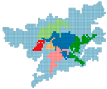 |
| SKATER | Minimum Bound | None Population: 100 to 1500 at intervals of 100 | None | 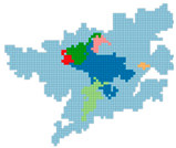 |
| Min region size | None Grids: 10 to 60 at intervals of 5 | None | ||
| REDCAP | Method | Full-Order Ward’s Linkage First-Order Single Linkage Full-Order Complete Linkage Full-Order Average Linkage Full-Order Single Linkage | Full Order Ward’s Linkage | 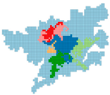 |
| Minimum Bound | None Population: 100 to 1500 at intervals of 100 | No impact | ||
| Min region size | None Grids: 10 to 60 at intervals of 5 | None | ||
| AZP | Minimum Bound | None Population: 100 to 1500 at intervals of 100 | 1000 | 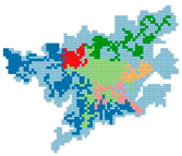 |
| Min region size | None Grids: 10 to 60 at intervals of 5 | No impact | ||
| Arisel | None, 10 to 100 at intervals of 10 | No impact | ||
| AZP-Tabu Search | Tabu length | 10, 15, 25, 50, 100, 300, 600, 1200 | 1200 | 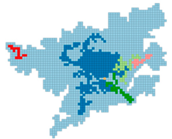 |
| AZP-Simulated Annealing | Cooling Rate | 0.70, 0.80, 0.85 | 0.70 | 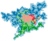 |
| MaxIt | 1, 3, 7 | 7 |
| Territory | Number of Clusters | Method | |||
|---|---|---|---|---|---|
| SCHC | SKATER | REDCAP | AZP | ||
| Vilnius | 6 | 0.549 | 0.455 | 0.556 | 0.572 |
| 7 | 0.560 | 0.467 | 0.564 | 0.603 | |
| 8 | 0.570 | 0.479 | 0.572 | 0.621 | |
| Kaunas | 6 | 0.586 | 0.531 | 0.579 | 0.627 |
| 7 | 0.597 | 0.543 | 0.595 | 0.640 | |
| 8 | 0.607 | 0.553 | 0.607 | 0.645 | |
| Klaipėda | 6 | 0.679 | 0.620 | 0.679 | 0.700 |
| 7 | 0.692 | 0.632 | 0.693 | 0.695 | |
| 8 | 0.702 | 0.642 | 0.703 | 0.699 | |
 |  |  |
| A. Clusters: 7 Minimum Bound: Population 1000 BSS/TSS = 0.603 | B. Clusters: 7 Minimum Bound: Population 1500 BSS/TSS = 0.625 | C. Clusters: 8 Minimum Bound: Population 1000 BSS/TSS = 0.621 |
| Territory | AZP Heuristic | ||
|---|---|---|---|
| Original | Tabu Search | Simulated Annealing | |
| Vilnius | 0.572 | 0.629 | 0.677 |
| Kaunas | 0.627 | 0.584 | 0.693 |
| Klaipėda | 0.700 | 0.684 | 0.719 |
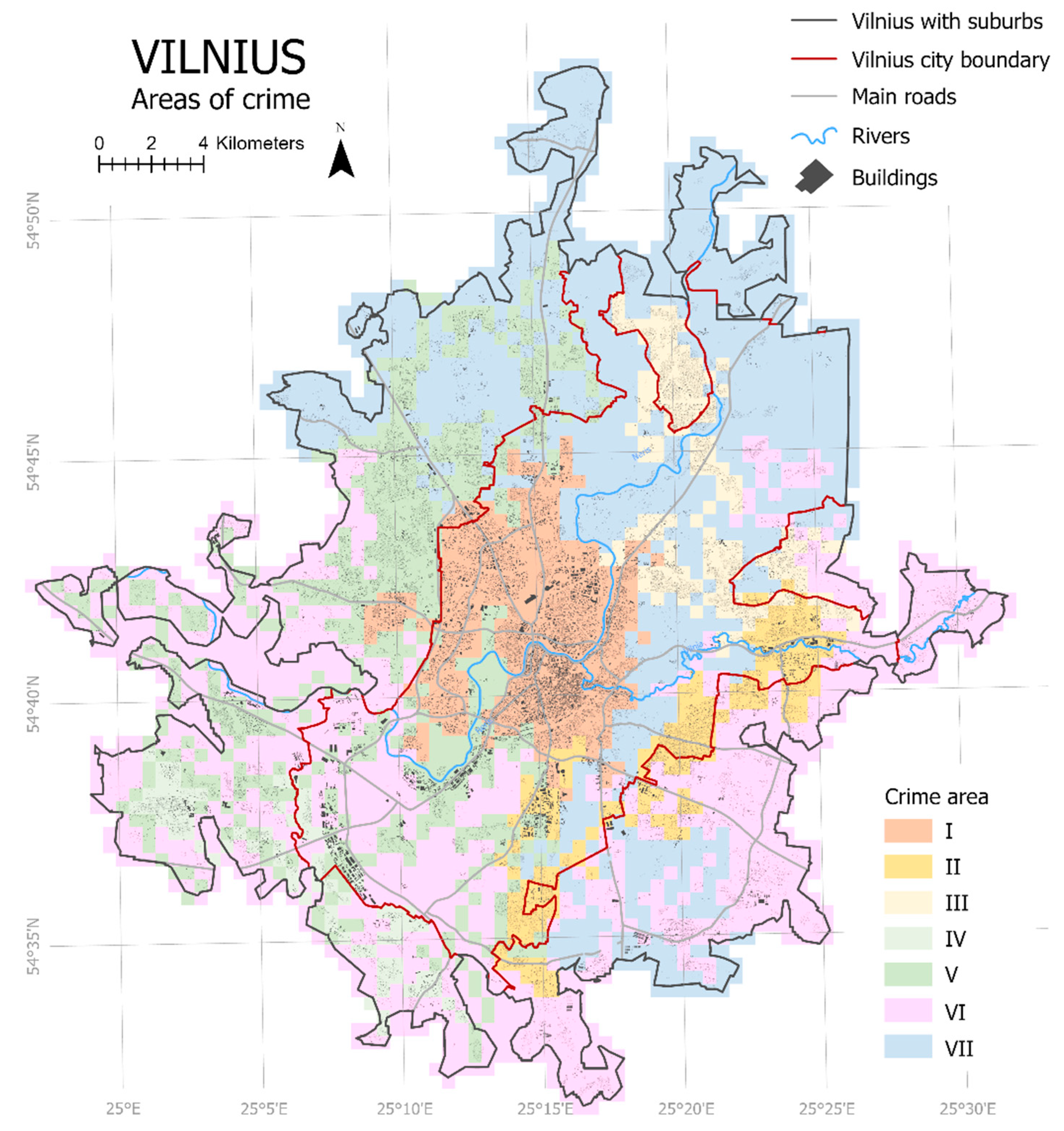
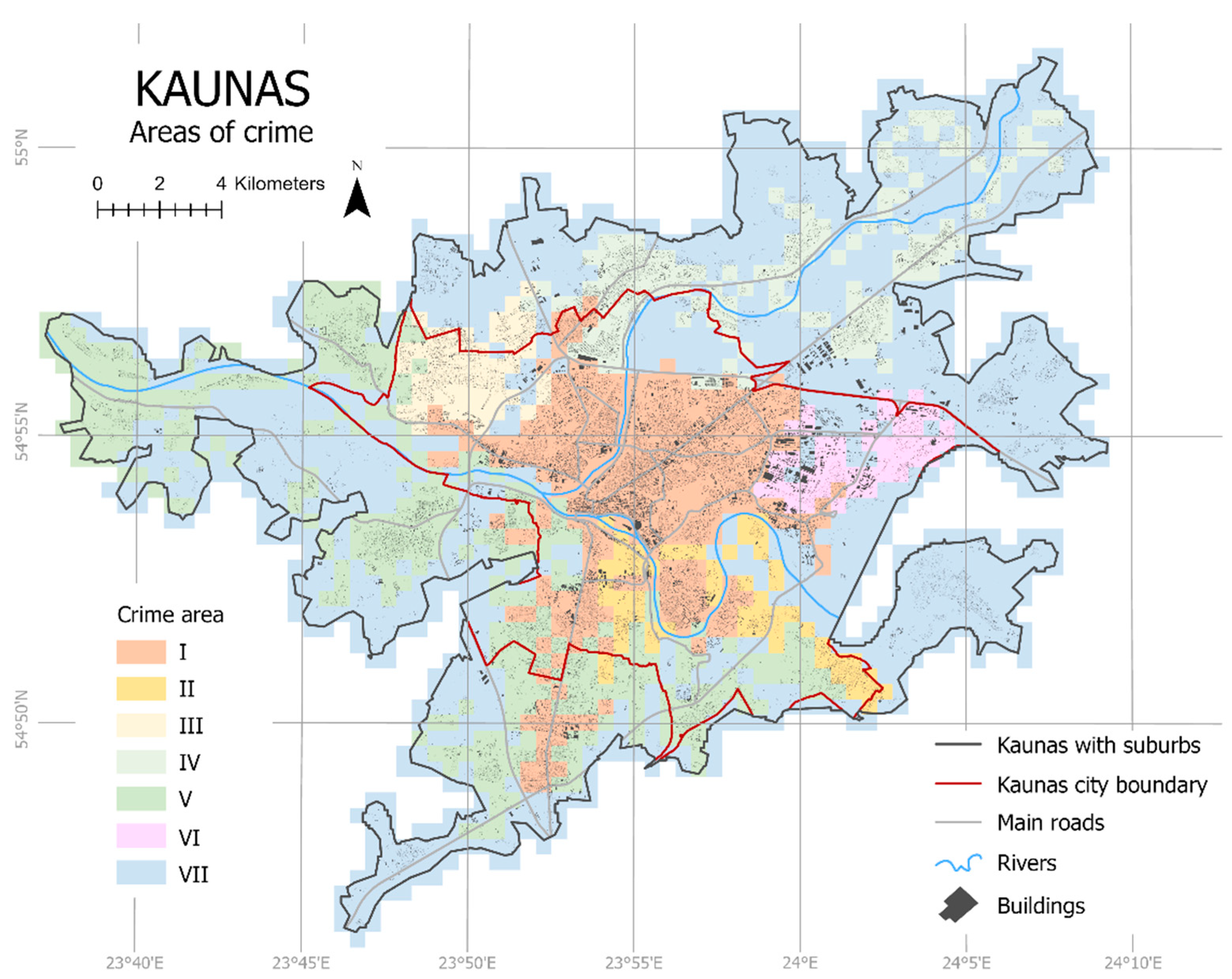
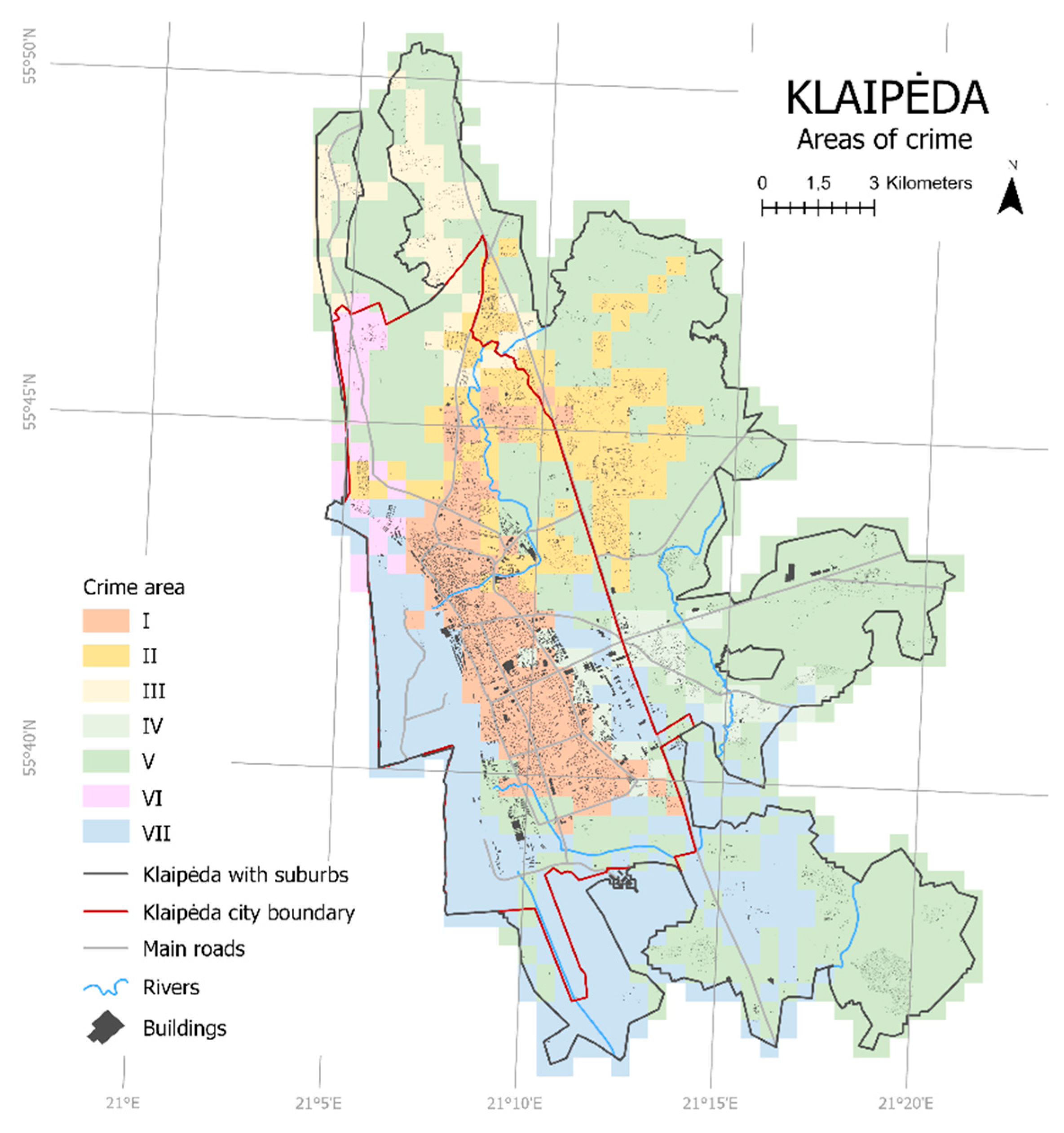
| Area of Crime | Characteristics of the Crime Area Specificity of Individual Cities | Corresponding Urban Socio-Demographic Type |
|---|---|---|
| I | Average crime rate, with all types of crime being proportional to population. Highest number of VIO. In Vilnius, a lower number of VIO events occur in open spaces than in the other two cities. | Central (historical) parts: medium population density, densely built-up with some derelict buildings and prevalence of SMEs’ commercial services. In Vilnius, this cluster also includes densely populated residential areas around the city centre. |
| II | Relatively high levels of crime, more in premises, larger proportion of IPP and PRO. In Vilnius, more VIO events, both in open spaces and in premises. In Klaipėda, generally lower crime rate. | Residential blocks of flats, densely built-up, high population density, commercial services of SMEs and large retail chains. Developed social infrastructure, such as schools, kindergartens, healthcare centres and interspersed green spaces. Intensive mobility of locals for daily needs around shopping centres. |
| III | Lower level of crime and predominance of crime on premises. In Vilnius, lower rate of IPP in open spaces. | Residential areas with detached houses within the city, medium population density, low level of commercialisation of the area and social control technologies (video surveillance, fences, gates used in the delineation of private property |
| IV | Large proportion of crimes in open spaces, especially VIO and IPP. In Vilnius, relatively more VIO events, both in open spaces and on premises. | Peripheral urban areas of mixed development (residential, medium and small business and manufacturing enterprises), lower than average population density and operational commercial structures. |
| V | Low-to-average levels of recorded crime, of which crime on premises predominate. In Vilnius, higher rates of PRO and IPP. | Single-family detached house areas in the suburbs and gated communities, with average and lower than average population densities. |
| VI | Relatively high number of VIO events, specifically in open spaces. In Kaunas, higher population density and high rates of PRO and IPP. | Sparsely populated areas with derelict buildings. Areas are being regenerated, and businesses are operating. These areas are designated for economic activities rather than for permanent residence. |
| VII | Below-average levels of recorded crime. Relatively higher number of IPP events in open spaces. In Klaipėda, virtually uninhabited areas; very high relative crime levels, especially of IPP in open spaces, are due to extremely sparse populations. | Settlements remote from the core urban area, which are within the economic pull of the metropolitan area due to the daily commuting of inhabitants. Average and below-average population density. |
Disclaimer/Publisher’s Note: The statements, opinions and data contained in all publications are solely those of the individual author(s) and contributor(s) and not of MDPI and/or the editor(s). MDPI and/or the editor(s) disclaim responsibility for any injury to people or property resulting from any ideas, methods, instructions or products referred to in the content. |
© 2023 by the authors. Licensee MDPI, Basel, Switzerland. This article is an open access article distributed under the terms and conditions of the Creative Commons Attribution (CC BY) license (https://creativecommons.org/licenses/by/4.0/).
Share and Cite
Beconytė, G.; Gružas, K.; Spiriajevas, E. Areas of Crime in Cities: Case Study of Lithuania. ISPRS Int. J. Geo-Inf. 2024, 13, 1. https://doi.org/10.3390/ijgi13010001
Beconytė G, Gružas K, Spiriajevas E. Areas of Crime in Cities: Case Study of Lithuania. ISPRS International Journal of Geo-Information. 2024; 13(1):1. https://doi.org/10.3390/ijgi13010001
Chicago/Turabian StyleBeconytė, Giedrė, Kostas Gružas, and Eduardas Spiriajevas. 2024. "Areas of Crime in Cities: Case Study of Lithuania" ISPRS International Journal of Geo-Information 13, no. 1: 1. https://doi.org/10.3390/ijgi13010001
APA StyleBeconytė, G., Gružas, K., & Spiriajevas, E. (2024). Areas of Crime in Cities: Case Study of Lithuania. ISPRS International Journal of Geo-Information, 13(1), 1. https://doi.org/10.3390/ijgi13010001