mapSR: A Deep Neural Network for Super-Resolution of Raster Map

Abstract

The purpose of multisource map super-resolution is to reconstruct high-resolution maps based on low-resolution maps, which is valuable for content-based map tasks such as map recognition and classification. However, there is no specific super-resolution method for maps, and the existing image super-resolution methods often suffer from missing details when reconstructing maps. We propose a map super-resolution (mapSR) model that fuses local and global features for super-resolution reconstruction of low-resolution maps. Specifically, the proposed model consists of three main modules: a shallow feature extraction module, a deep feature fusion module, and a map reconstruction module. First, the shallow feature extraction module initially extracts the image features and embeds the images with appropriate dimensions. The deep feature fusion module uses Transformer and Convolutional Neural Network (CNN) to focus on extracting global and local features, respectively, and fuses them by weighted summation. Finally, the map reconstruction module uses upsampling methods to reconstruct the map features into the high-resolution map. We constructed a high-resolution map dataset for training and validating the map super-resolution model. Compared with other models, the proposed method achieved the best results in map super-resolution.

1. Introduction

Earth observation systems and big data techniques gave birth to the exponential growth of large amounts of professionally generated and volunteered raster maps of various formats, themes, styles, and other attributes. As a great number of activities, including land cover/land use mapping [1], navigation [2], trajectory analysis [3], socio-economic analysis [4], etc., benefit from the geospatial information included in these raster maps, precisely retrieving the massive map dataset has become a pressing task. Traditional approaches for map retrieval, such as online search engines, generally rely on map annotations or the metadata of map files rather than the map content. These map annotations assigned to a raster map might vary due to subjective understanding as well as diverse map generation goal, map themes, and other factors [5]. In comparison to map annotations and metadata, content-based map retrieval mainly focuses on employing the information included in a map to determine whether the retrieved map is truly needed by the user or for a task. Map text and symbols are the first map language and the essential part of map features with respect to map content [6,7,8]. Thus, map text and symbol recognition has become a main research aspect of big map data retrieval. Recently, deep learning techniques such as convolutional neural networks (CNNs) have shown great strengths in map text and symbol recognition. Furthermore, Zhou et al. [9] and Zhou [10] reported that deep learning approaches could effectively support the retrieval of topographical and raster maps by recognizing text information.

However, poor spatial resolution and limited data size remain the two main obstacles for implementing state-of-the-art deep learning approaches into map text and symbol recognition. In the era of big data and volunteered geographical information, a majority of available maps are designed and created in unprofessional ways. This always makes the text characters and symbols in these maps unavailable for visual recognition due to poor spatial resolution or small data size.

Super-resolution techniques support the conversion of low-resolution images into high-resolution ones by extracting the mappings between low-resolution images and their corresponding high-resolution ones. Super-resolution techniques include multi-frame super-resolution (MFSR) and single-image super-resolution (SISR) [11,12]. Considering that the generation of a map is always time-consuming, generating multiple types of maps that share a similar theme or style is generally impossible on the raster. Thus, SISR would be useful for research in map reconstruction. Currently, the community of machine intelligence and computer vision reported that CNNs have achieved great success in SISR [13,14]. However, due to the limited receptive field of convolution kernels, it is difficult to effectively utilize global features. Moreover, although increasing the network depth can expand the receptive field of CNNs to some extent, this strategy still cannot fundamentally solve the receptive field in the spatial dimension. Specifically, increasing the depth might lead to an edge effect—the reconstruction of image edges is significantly worse than in the middle of the image. Otherwise, vision transformer (ViT) mainly focuses on modeling the features of the global receptive field using the attention mechanism [15].

Unlike natural images, maps contain a variety of information on different scales, containing both geographical information with global features and detailed information such as legends and annotations. The former follows Tobler’s first law of geography and consists mainly of low-frequency information being available for reconstruction using Transformer for global modeling. The latter has a large amount of high-frequency information and requires the use of CNN modules to focus on reconstructing the local details of maps. Up to now, super-resolution methods that fuse global and local information for maps have not been reported.

To deal with the super-resolution reconstruction of maps, we propose a mapSR model using a Transformer backbone with a fusion of CNN modules that focus on extracting local features. Experiments proved that our model was better than other models in the super-resolution reconstruction of maps.

The remainder of this paper is organized as follows. Section 2 briefly reviews the progress of SISR based on deep learning. Section 3 presents our proposed method for low-resolution map reconstruction. Section 4 describes experiments to evaluate the performance of our proposed model in low-resolution map reconstruction. Section 5 summarizes the contributions of this paper.

2. Related Works

2.1. CNN-Based SR

CNNs have been used for a long time. In the 1990s, LeCun et al. [16] proposed LeNet using the backpropagation algorithm, which initially established the structure of CNNs. Dong et al. proposed the first super-resolution network, SRCNN [17], in 2014, which achieved results beyond previous traditional interpolation methods by using only three layers of convolution. As a pioneering work to introduce CNN into super-resolution, SRCNN had the problem of limited learning ability due to the shallow network, but it established the basic structure of image super-resolution, that is, the three-level structure of feature extraction, nonlinear mapping, and high-resolution reconstruction. They further proposed FSRCNN [18] in 2016, where they moved the upsampling layer back, allowing feature extraction and mapping to be performed on low-resolution images, they used several small convolutions instead of a large convolution, both of which reduced the computations, and they replaced the upsampling method from interpolation to transposed convolution, which enhanced the learning ability of the model.

ESPCN [19], VDSR [20], DRCN [21], and LapSRN [22] were proposed to improve the existing super-resolution models from different perspectives. ESPCN proposed a PixelShuffle method for upsampling, which was proven to be better than transposed convolution and interpolation methods and has been widely used in later super-resolution models. Inspired by ResNet and RNN, Kim et al. proposed two methods, VDSR and DRCN, to deepen the model and improve the feature extraction ability. LapSRN was proposed as a progressive upsampling method, which was faster and more convenient for multi-scale reconstruction than single upsampling.

Lim et al. [23] found that the Batch Normal (BN) layer normalized the image color and destroyed the original contrast information of the image, which hindered the convergence of training. Therefore, they proposed EDSR to remove the BN layer, implement a deeper network, and proposed residual scaling to solve the problem of numerical instability in the training process caused by the overly deep network. Inspired by DenseNet, Haris et al. [24] proposed DBPN, which proposed an iterative upsampling and downsampling process that provided an error feedback mechanism for each stage and achieved excellent results in large-scale image reconstruction.

2.2. Transformer-Based SR

In 2017, Ashish et al. [25] first proposed the Transformer model for machine translation using stacked self-attention layers and fully connected layers (MLP) to replace the circular structure of the original Seq2Seq. Because of the great success of Transformer in NLP, Kaiser et al. [26] soon introduced it to image generation work, and Alexey et al. [27] proposed Vision Transformer (ViT), which segmented images into blocks and then serialized them, using Transformer to implement image classification. In recent years, Transformer, especially ViT, has gradually attracted the attention of the SISR academic community.

RCAN [28] introduced Transformer to image super-resolution and proposed a channel attention (CA) mechanism that adaptively adjusted features considering the dependencies between channels, further improving the expressive capability of the network compared to CNN. Dai et al. [29] proposed a second-order channel attention mechanism to better adaptively adjust the channel features considering that the global covariance could obtain higher-order and more discriminative feature information compared with the first-order pooling used in RCAN.

Inspired by Swin Transformer, Liang et al. [30] proposed SwinIR, which used window partitioning to obtain several local windows, Transformer was used in each window, and the information across windows was fused by window shifting at the next layer. This solution of implementing Transformer for partitioned windows could greatly reduce the computations, had the advantage of processing larger sized images, and also could take advantage of Transformer by shifting windows to achieve modeling of the global dependency. Considering that the window partitioning strategy of SwinIR limited the receptive field and could not establish long dependencies at an early stage, Zhang et al. [31] used a fast Fourier convolutional layer with a global receptive field to extend SwinIR, while Chen et al. [15] combined SwinIR with a channel attention mechanism to propose a hybrid attentional Transformer model. Both approaches enabled SwinIR to establish long dependencies at the early stage and improved model performance using different methods.

Transformer breaks away from the dependence on convolution by using an attention mechanism and has a global receptive field, which can achieve better image super-resolution results compared to CNN. However, Transformer does not have the capability of capturing local features and is not sensitive enough to some local details of maps. Therefore, a Transformer model that fuses local features may be more effective for map super-resolution.

3. Framework of mapSR

Map content is always represented by features at global and local scales. Global features mainly refer to the overall color distribution and brightness of the map, while local features mainly refer to the texture, edges, and corner details in the map. These features would be critical for reconstructing map text, map symbols, map scenes, and other map elements. We propose a network (mapSR) for super-resolution reconstruction of low-resolution maps, which integrates the global and local information of maps. The network combines the global and local information extracted by Swin Transformer and CNN, respectively. The specific structure is shown in Figure 1a. The proposed model consists of three modules: a shallow feature extraction module, a deep feature fusion module, and a map reconstruction module. The shallow feature extraction module focuses on employing convolutional and pooling layers to extract the features from a raster map. The deep feature fusion module uses the residual feature fusion group to fuse the global and local features of the map. Based on the fused features, the map reconstruction module exploits Pixel-Shuffle for generating the super-resolution result.

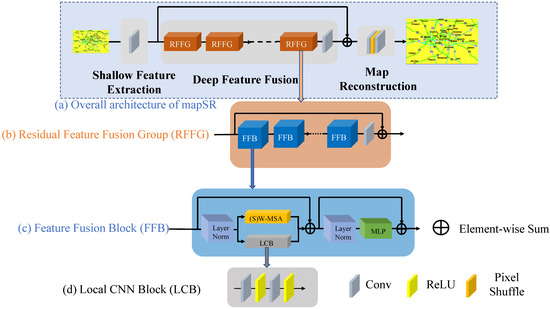
Figure 1. The framework of mapSR network.

3.1. Shallow Feature Extraction Module

For a given low-resolution (LR) map input $I_{LR}\in {ℝ}^{H\times W\times C_{in}}$, $H$, $W$, and $C_{in}$ respectively refer to the horizontal dimension, vertical dimension, and channel number of the input map. We first used a layer of convolution to extract its shallow features $F_0\in {ℝ}^{H\times W\times C}$ by the following equation:

$$F_0=H_{SF}(I_{LR})$$

(1)

where $C$ refers to the dimension of the shallow feature extraction module. The shallow features of maps are represented by $F_0$, which includes basic and localized feature information (such as edges and lines) extracted by a simple CNN layer, and can be used for subsequent deep feature extraction. $H_{SF}(\cdot )$ refers to the shallow feature extraction module, which consists of a simple 3 × 3 convolutional layer.

3.2. Deep Feature Fusion Module

3.2.1. Attentions with Feature Fusion Blocks

Based on the shallow features, depth feature fusion $H_{DF}(\cdot )$ was performed to obtain the deep features $F_{DF}\in {ℝ}^{H\times W\times C}$ by the following equation:

$$F_{DF}=H_{DF}(F_0)$$

(2)

$H_{DF}(\cdot )$ contained N residual feature fusion groups (RFFG) and a 3 × 3 convolutional layer, which could be expressed as follows. In this paper, we took N = 6.

$$\left\{\begin{array}{l}{F}_i=H_{RFF{G}_i}(F_{i-1}),i=1,2,\dots ,N\\ F_{DF}=H_{Conv}(F_N)\end{array}\right.$$

(3)

where $H_{RFF{G}_i}(\cdot )$ denotes the $i$-th RFFG and $H_{Conv}(\cdot )$ denotes the convolutional layer, which can better aggregate the previously fused features. The architecture of RFFG is shown in Figure 1b. Each RFFG contained M feature fusion blocks (FFB) and a 3 × 3 convolutional layer. In this paper, we took M = 6.

Here, we proposed FFB to fuse the features within local details derived from the CNNs and the global features derived from the Transformer. The architecture of FFB is shown in Figure 1c. The backbone was the standard Swin Transformer module. We employed the local CNN block (LCB) to extract local-detail features and the window-based multi-head self-attention (W-MSA) and the shifted window-based multi-head self-attention (SW-MSA) to extract global-scale features. Then, we used layer normalization and MLP to fuse the global and local features via weighted summation.

The overall process can be formulated as follows:

$$\left\{\begin{array}{l}{X}_N=LN(X)\\ X_M=\left(\mathrm{S}\right)\mathrm{W}-\mathrm{MSA}(X_N)+\alpha LCB(X_N)+X\\ Y=MLP(LN(X_M))+X_M\end{array}\right.$$

(4)

where $X$ refers to the input features of FBB and $Y$ refers to the fused features. $LN(\cdot )$ and $MLP(\cdot )$ respectively denote the LayerNorm layer and the multi-layer perceptron.

The structure of LCB is shown in Figure 1d, which includes two 3 × 3 convolutional layers, each followed by a ReLU activation function, as shown in Figure 1d. The whole process is formulated as follows:

$$X_{out}=\mathrm{ReLU}(Con{v}_2(\mathrm{ReLU}(Con{v}_1(X_{in}))))$$

(5)

where $X_{in}$, $X_{out}$, $Con{v}_1$, and $Con{v}_2$ represent the input features, output features, and two convolutional layers, respectively.

Moreover, W-MSA and SW-MSA were used in FFBs, and a weighting factor α was given to the output features of the LCB to avoid possible conflicts in fusing global features with local features.

For the (S)W-MSA module, given an input feature of dimension $H\times W\times C$, we partitioned it into $HW/M^2$ local windows within the dimension of $M\times M$. Thus, the feature generated from each window is $X_W\in {ℝ}^{M\times M\times C}$.

Then, we conducted self-attention for each window. For each local window feature, the query ($Q$), key ($K$), and value ($V$) were first obtained via a nonlinear mapping, and the window self-attention is formulated as:

$$\mathrm{Attention}(Q,K,V)=\mathrm{SoftMax}(Q{K}^T/\sqrt{d}+B)V$$

(6)

where $d$ denotes the dimension of query and key, and $B$ represents the relative position encoding. $\mathrm{SoftMax}$ refers to the activation function.

3.2.2. Attention Partition with Shifted Window

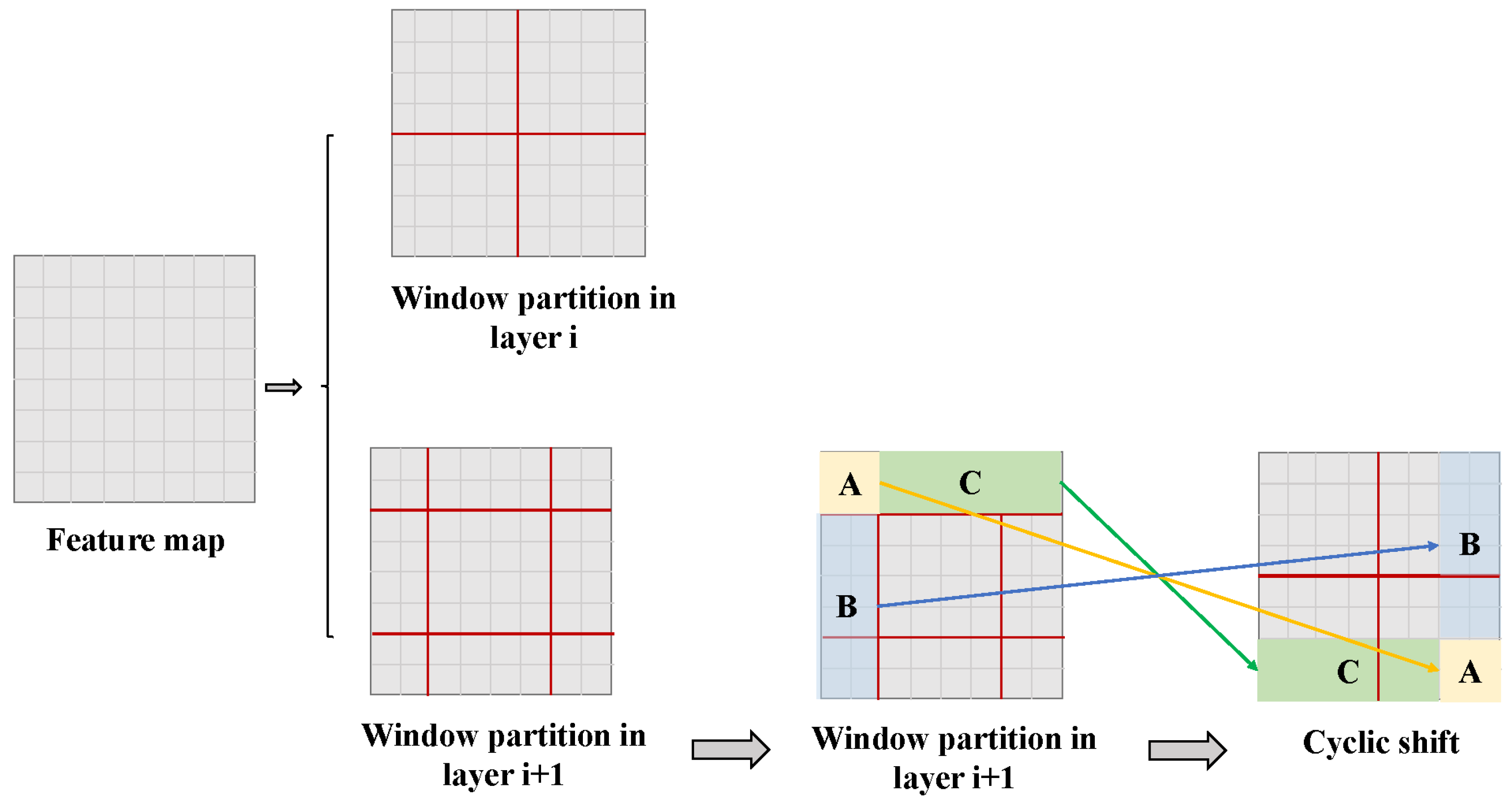
Spatial partitioning could influence feature learning by an attention mechanism. As shown in Figure 2, W-MSA and SW-MSA adopt different window partitioning strategies; they are used alternately in FFBs to obtain the global features from every part of the image.

Figure 2. Window partitioning strategy for (S)W-MSA. A, B and C respectively denotes the top-left corner window, the left window, and the top window used for partition.

Above of all, based on Equation (1), for the $i$-th RFFG, we could have the following expression:

$$\left\{\begin{array}{l}{F}_{i-1,0}=F_{i-1}\\ F_{i-1,j}=H_{FFB}(F_{i-1,j-1}),j=1,2,\dots ,M\\ F_i=H_{Con{v}_i}(F_{i-1,M})+F_{i-1}\end{array}\right.$$

(7)

where $F_{i-1,0}$ indicates the input features of the $i$-th RFFG and $F_{i-1,j}$ represents the output features of the $j$-th FFB in the $i$-th RFFG. After several FFBs, we also used a convolutional layer to aggregate features and residual connections, thereby ensuring the stability of the training process.

3.3. Map Reconstruction

Meanwhile, considering that low- and high-resolution maps contain much of the same low-frequency information, to make the deep feature fusion module focus on modeling the high-frequency detailed information, we used a residual connection to fuse the shallow features with the deep features, and finally reconstructed the high-resolution map via a map reconstruction module, as:

$$I_{SR}=H_{\mathrm{Re}c}(F_0+F_{DF})$$

(8)

where $H_{\mathrm{Re}c}(\cdot )$ indicates the map reconstruction module. Specifically, we used the PixelShuffle method to upsample the fused features.

4. Experiments and Discussion

4.1. Experimental Dataset and Implementation

We constructed a map dataset for training the map super-resolution model. The dataset contained a total of 668 high-resolution raster maps, with 600, 60, and 8 maps in the training set, validation set, and test set, respectively. Bicubic interpolation was used to downsample each map to obtain its corresponding low-resolution map. Figure 3A shows the selected original (high-resolution) map samples, and Figure 3B shows the results of super-resolution reconstruction including the original (high-resolution) maps and the low-resolution maps obtained by downsampling. Additionally, “Original,” “Downsample:1/2,” and “Downsample:1/3” respectively denote the original maps, the maps generated by 2X downsampling, and the maps generated by 3X downsampling. Moreover, as mentioned in the Introduction, deep learning regarding super-resolution is fit for dealing with maps generated by cartographical principles and extracting geospatial information from unprofessionally produced maps is a big challenge. In this manuscript, all of the maps shown in Figure 3 were collected from ubiquitous sources, which means that these unprofessionally produced maps did not follow cartographical principles. Thus, the scale bars were not available in these maps.

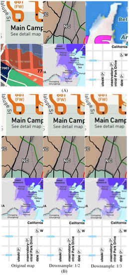
Figure 3. (A) Original raster maps for testing and training. (B) Low-resolution raster maps obtained by downsampling.

The dataset can be accessed from the following link: https://pan.baidu.com/s/15999TSy6siHCeorL1DXH1A?pwd=u0cx (accessed on 19 June 2023).

To evaluate the model’s performance, our model was compared with state-of-the-art CNN-based super-resolution models (EDSR and DBPN) and Transformer-based super-resolution models (RCAN and SwinIR). All models are available at the following links.

• EDSR: https://github.com/sanghyun-son/EDSR-PyTorch (accessed on 19 June 2023)
• DBPN: https://github.com/alterzero/DBPN-Pytorch (accessed on 19 June 2023)
• RCAN: https://github.com/yulunzhang/RCAN (accessed on 19 June 2023)
• SwinIR: https://github.com/JingyunLiang/SwinIR (accessed on 19 June 2023)

We trained all models on PyTorch by optimizing these models with the L1 loss function, setting the initial learning rate to 1.0 × 10⁻⁴, and dynamically adjusting the learning rate by the cosine annealing algorithm. Moreover, peak signal-to-noise ratio (PSNR) and structural similarity (SSIM) are commonly used metrics in image super-resolution reconstruction for indicating how similar the reconstructed image is to the original high-resolution image [17,20,21,22,23]. Thus, we employed PSNR and SSIM to quantitatively evaluate the performance of each approach. PSNR and SSIM are expressed as follows:

$$\left\{\begin{array}{l}MSE=\frac{1}{XY}\times {\displaystyle \sum _{a=1}^X{\displaystyle \sum _{b=1}^Y{(I_t(a,b)-I_r(a,b))}^2}}\\ PSNR=10\times {\log }_{10}\frac{{255}^2}{MSE}\end{array}\right.$$

(9)

where $MSE$ denotes the mean square error. $I_t$ and $I_r$ are the test image after super-resolution and the referenced image, respectively. $I_t(a,b)$ and $I_r(a,b)$ denote where the pixel is located $(a,b)$ in the test image and the referenced image. $X$ and $Y$ are the horizontal and vertical dimensions, respectively, of the test image and the referenced image. Accordingly, the unit of PSNR is dB. Larger PSNR values mean lower distortion after super-resolution.

SSIM measures the similarity between a test image and its corresponding referenced image based on three aspects, brightness, contrast, and structure, which are expressed in the following equations:

$$\left\{\begin{array}{l}BRG=\frac{2\times mea{n}_t\times {mean}_r+{\sigma }_1}{{\left(mea{n}_t\right)}^2+{\left(mea{n}_r\right)}^2+{\sigma }_1}\\ CTR=\frac{2\times {\mathrm{var}}_t\times {\mathrm{var}}_r+{\sigma }_2}{{\left({\mathrm{var}}_t\right)}^2+{\left({\mathrm{var}}_r\right)}^2+{\sigma }_2}\\ STR=\frac{{\mathrm{cov}}_t+{\sigma }_2}{{\mathrm{var}}_t\times {\mathrm{var}}_r+{\sigma }_3}\end{array}\right.$$

(10)

where $BRG$, $CTR$, and $STR$ refer to brightness, contrast, and structure, respectively. $\mathrm{M}\mathrm{e}\mathrm{a}\mathrm{n}$, $\mathrm{v}\mathrm{a}\mathrm{r}$, and $\mathrm{c}\mathrm{o}\mathrm{v}$ denote the mean and variance of an image and the covariance of two images, respectively. Moreover, ${\sigma }_1$, ${\sigma }_2$, and ${\sigma }_2$ are independent constants, which are calculated by the following equations:

$$\left\{\begin{array}{c}{\sigma }_1={({\theta }_1\times 255)}^2\\ {\sigma }_2={({\theta }_2\times 255)}^2\\ {\sigma }_3=\frac{{\sigma }_2}{2}\end{array}\right.$$

(11)

where the values of ${\theta }_1$ and ${\theta }_2$ depend on the map content. Generally, we assign 0.01 and 0.03 to ${\theta }_1$ and ${\theta }_2$, respectively. SSIM is then calculated by multiplying brightness, contrast, and structure.

$$SSIM=BRG\times CTR\times STR$$

(12)

The experiments were carried out using NVIDIA GeForce RTX 2070 Ti GPUs. The Adam optimizer was employed to optimize the model parameters, with Adam optimizer parameters ${\mathsf{\beta }}_1$ = 0.9 and ${\mathsf{\beta }}_2$ = 0.999. The training process consisted of four phases, each with a different number of iterations: 50 K, 50 K, 100 K, and 100 K. The initial learning rate was set to 1 × 10⁻⁴, and it was adjusted using the cosine annealing method, where the restart weights were assigned as follows: 1, 0.5, 0.5, and 0.25, respectively. The batch sizes for the experiments were set to 4 (2x) and 2 (3x), respectively.

4.2. Results and Discussions

4.2.1. Quantitative Results

Table 1 respectively presents the selected super-resolution results by different approaches based on the PSNR and SSIM values. We highlighted the best results in bold. X2 and X3 denote the scale regarding unsampling the original raster map.

Table 1. Comparison of PSNR values for different models.

Map	Scale	EDSR	DBPN	RCAN	SwinIR	mapSR
1	X2	33.4192	33.0892	34.0426	34.1651	34.0485
2		32.8611	32.9120	34.6523	34.1132	34.6985
3		28.6268	29.0341	30.2361	28.8198	30.1735
4		34.8944	34.7906	35.0431	34.8981	35.2994
5		29.8561	29.7685	30.4396	30.2846	30.5670
6		32.8816	33.1306	34.5478	34.1370	34.8909
7		38.8024	38.8269	42.3373	41.0826	43.3763
8		33.4507	33.6415	36.8867	34.5898	37.0953
avg.		33.0990	33.1492	34.7732	34.0113	35.0187
1	X3	29.4432	29.7042	29.9781	30.5131	29.6464
2		28.6196	29.1155	29.1369	29.0834	30.6319
3		23.0056	23.9230	24.6834	22.7049	24.9065
4		30.0887	30.2688	30.5821	30.7422	30.7725
5		25.0961	25.1343	25.9240	26.4909	26.3618
6		27.9597	28.3543	28.7026	27.9801	29.0721
7		30.8867	31.9362	33.3526	31.1853	34.7123
8		26.2006	27.8731	29.1660	25.5936	30.4279
avg.		27.6625	28.2887	28.9407	28.0367	29.5664
1	X2	0.9565	0.9551	0.9546	0.9572	0.9559
2		0.9591	0.9591	0.9591	0.9598	0.9595
3		0.9160	0.9162	0.9165	0.9164	0.9182
4		0.9516	0.9512	0.9493	0.9506	0.9509
5		0.8959	0.8949	0.8964	0.8969	0.8973
6		0.9505	0.9506	0.9494	0.9522	0.9522
7		0.9960	0.9953	0.9984	0.9978	0.9987
8		0.9939	0.9942	0.9979	0.9961	0.9982
avg.		0.9524	0.9521	0.9527	0.9534	0.9538
1	X3	0.9295	0.9318	0.9311	0.9368	0.9221
2		0.9318	0.9355	0.9356	0.9357	0.9348
3		0.8450	0.8544	0.8625	0.8421	0.8554
4		0.9172	0.9192	0.9194	0.9201	0.9177
5		0.8233	0.8282	0.8320	0.8329	0.8273
6		0.9172	0.9194	0.9214	0.9184	0.9230
7		0.9844	0.9880	0.9914	0.9825	0.9940
8		0.9726	0.9822	0.9866	0.9663	0.9926
avg.		0.9151	0.9198	0.9225	0.9168	0.9208

From the quantitative results listed in Table 1, several conclusions could be drawn. First, in general, RCANS and SwinIR outperformed EDSR and DBPN, meaning that the Transformer-based methods generally outperform the CNN-based ones. In addition, the results generated by RCAN and SwinIR were close to each other. Since RCAN and SwinIR respectively improve the initial vision transformer (ViT) by rescaling the channel features and the spatial features, we might conclude that both channel and spatial features could be useful for map super-resolution. Specifically, it is difficult to claim which feature would be more efficient. Finally, compared with the results of RCAN and SwinIR, our method improved the PSNR value by 0.2–1.0 dB at 2x super-resolution and by 0.6–1.5 dB at 3x super-resolution, proving that our proposed method could effectively enhance map super-resolution, and the improvement was more obvious for larger-scale map reconstruction. This meant that the fusion of local and global features could significantly improve the results of map super-resolution.

To verify the scalability of our proposed model, we conducted an additional experimental test including 500 maps. The detailed information regarding the experiment with 500 maps can be accessed at the following link: https://pan.baidu.com/s/1sfwfkBfgCLJAUX2alqYGGQ?pwd=lhh1 (accessed on 19 June 2023). It contains the testing set consisting of 500 maps and the corresponding 2x and 3x downsampled images, the results of the above experiments, and the experiment log.

Table 2 reveals that the minimum PSNR values for the reconstructed results of various models were relatively similar. However, the maximum PSNR values achieved by RCAN and mapSR significantly surpassed those of the other methods. Moreover, both RCAN and mapSR exhibited higher variance compared to the other methods. This phenomenon could be attributed to the presence of maps with substantial missing information, which posed a reconstruction challenge for all models. On the other hand, for maps with the majority of information retained, RCAN and mapSR demonstrated superior feature extraction capabilities, enabling them to achieve better reconstruction results. Moreover, to verify the efficiency of our proposed LCB in fusing local features, we generate various results by setting different weights α = 1, 0.1, and 0.01, and α = 0 (SwinIR) and evaluated these results based on the PSNR and SSIIM values. The results are shown in Table 2.

Table 2. PSNR and SSIM results on test_set_500.

PSNR		EDSR	DBPN	RCAN	SwinIR	mapSR
X2	min	25.1995	25.6105	25.9346	25.1513	26.1057
	max	42.3900	43.1568	48.1815	42.7556	46.6624
	mean	33.0666	33.8289	35.4099	33.3637	35.4836
	var	14.6673	14.6019	17.6664	15.7346	17.9187
X3	min	19.3009	20.3305	22.4703	20.1624	23.1906
	max	37.7150	38.0387	39.2920	38.0245	39.6565
	mean	27.9724	28.9612	30.0894	27.9687	30.6727
	var	12.5503	12.9635	13.9614	12.7918	14.7665
SSIM		EDSR	DBPN	RCAN	SwinIR	mapSR
X2	min	0.7051	0.7092	0.7135	0.7069	0.7143
	max	0.9985	0.9988	0.9994	0.9988	0.9993
	mean	0.9667	0.9700	0.9751	0.9685	0.9754
	var	0.0011	0.0010	0.0009	0.0011	0.0009
X3	min	0.6053	0.6120	0.6177	0.6068	0.6207
	max	0.9942	0.9957	0.9973	0.9947	0.9980
	mean	0.9182	0.9300	0.9402	0.9209	0.9462
	var	0.0043	0.0038	0.0033	0.0040	0.0030

As listed in Table 3, the results generated by the proposed method with different LCB weights outperformed the results generated by SwinIR. This proved the validity of LCB in fusing local and global features. Moreover, we also found that a small weighting factor always led to a better result, meaning that increasing the weight of the CNN module would decrease the performance of map reconstruction. This indicated that optimization of the CNN module and self-attention still had challenges to be addressed.

Table 3. Comparison of PSNR for different LCB weights.

Map	SwinIR (α = 0)	mapSR (α = 0.01)	mapSR (α = 0.1)	mapSR (α = 1.0)
1	34.1651	34.0485	34.1574	34.0989
2	34.1132	34.6985	34.7030	34.6605
3	28.8198	30.1735	29.9528	29.9388
4	34.8981	35.2994	35.3150	35.3195
5	30.2846	30.5670	30.5625	30.5608
6	34.1370	34.8909	34.8191	34.8402
7	41.0826	43.3763	42.8437	42.8933
8	34.5898	37.0953	36.7510	36.4225
avg.	34.0113	35.0187	34.8880	34.8418
1	0.9572	0.9559	0.9563	0.9559
2	0.9598	0.9595	0.9599	0.9596
3	0.9164	0.9182	0.9180	0.9177
4	0.9506	0.9509	0.9511	0.9510
5	0.8969	0.8973	0.8975	0.8974
6	0.9522	0.9522	0.9519	0.9518
7	0.9978	0.9987	0.9985	0.9985
8	0.9961	0.9982	0.9979	0.9978
avg.	0.9534	0.9538	0.9539	0.9537

Similarly, we performed the above ablation experiment on test_set_500 with the following results.

As listed in Table 4, this fusion module could greatly improve the reconstruction when using smaller fusion coefficients, which was due to the fusion of global and local information processed by mapSR. Moreover, the performance of mapSR was proportional to the value of the fusion coefficients, which might have been due to the phenomenon that a CNN module with a larger weight could not effectively use the global information of the image.

Table 4. Results of ablation experiments on test_set_500.

		SwinIR (α = 0)	mapSR (α = 0.01)	mapSR (α = 0.1)	mapSR (α = 1.0)
x2	PSNR	33.3637	35.4836	35.4463	32.6522
	SSIM	0.9685	0.9754	0.9753	0.9642
x3	PSNR	27.9687	30.6727	30.6639	28.6836
	SSIM	0.9209	0.9462	0.9460	0.9254

4.2.2. Visual Results

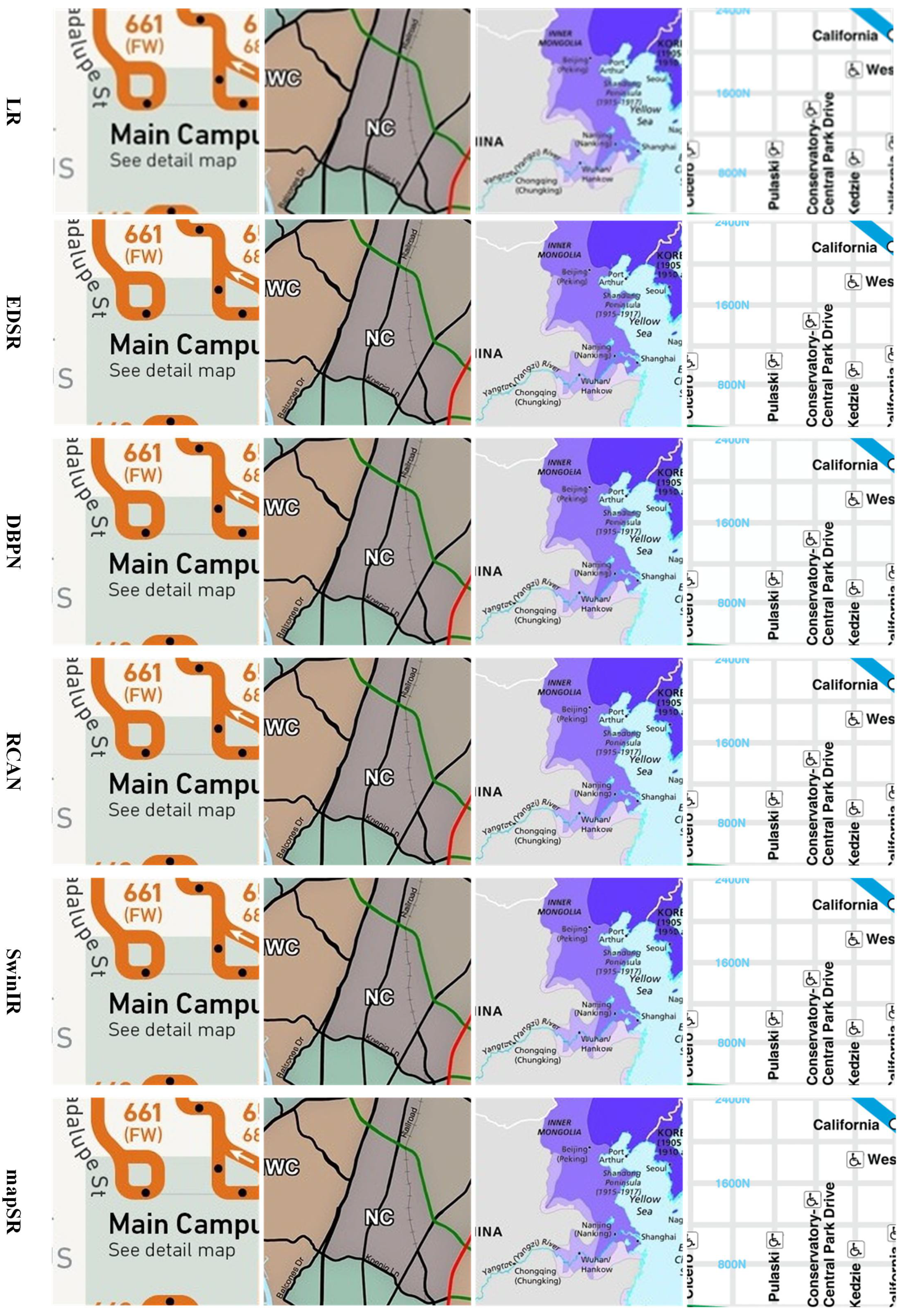
Figure 4 and Figure 5 provide a visual comparison of the results generated by all models. Figure 4 shows the results of the 2x super-resolution reconstruction, and it is clear that the Transformer-based model achieved significantly better results than the CNN-based model, and that our method reconstructed many local details better than the other methods.

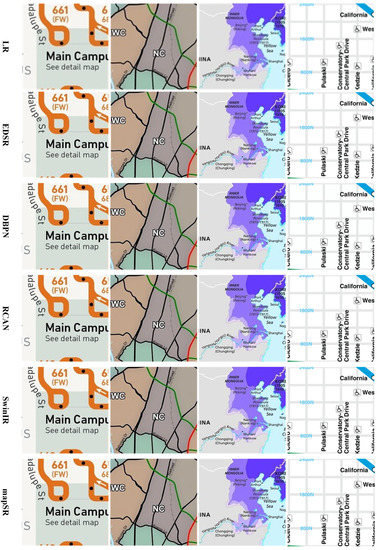
Figure 4. Comparison of 2X map reconstruction results by various SISR models.

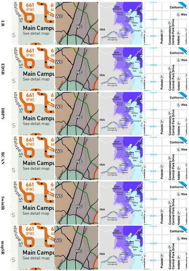
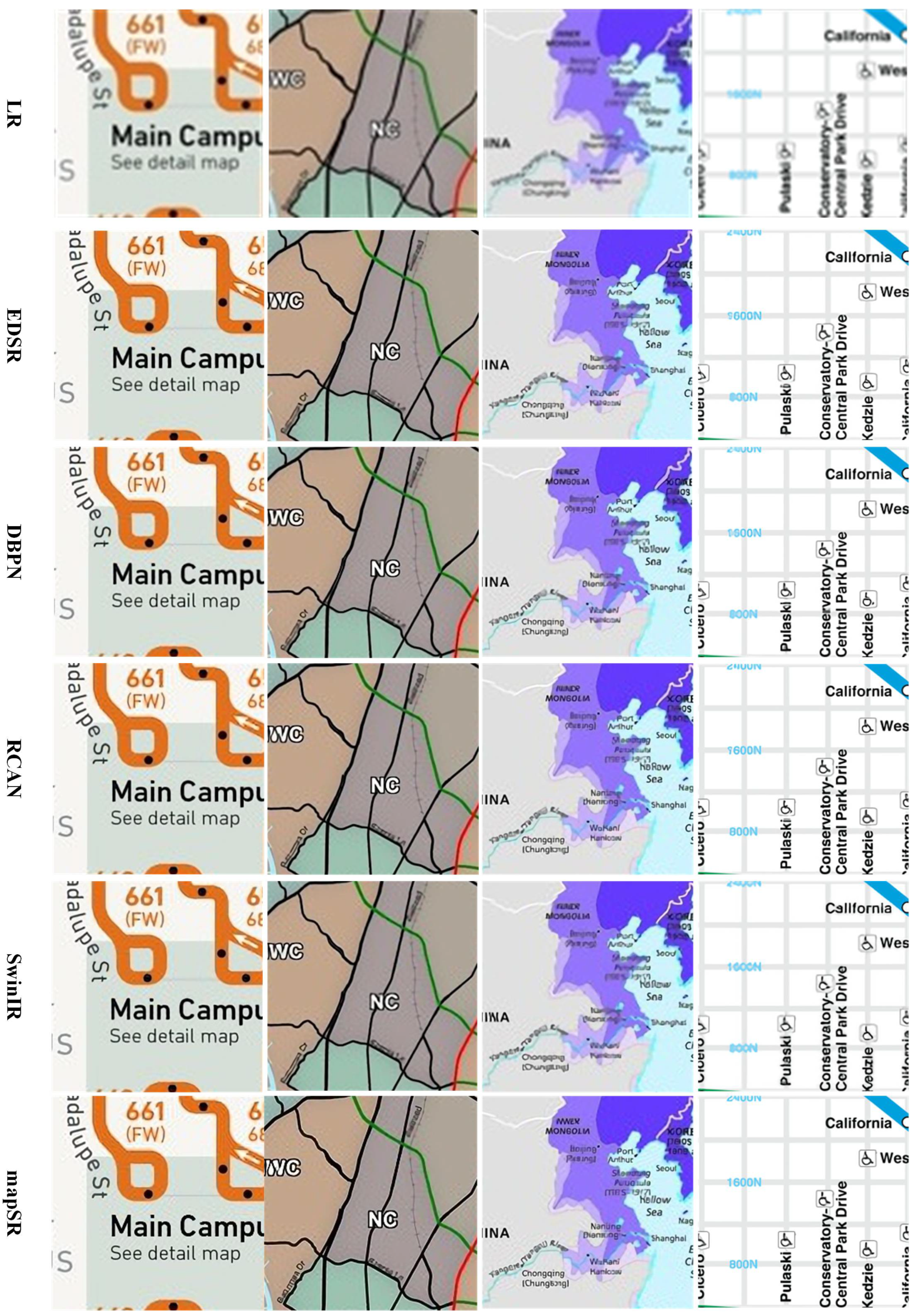
Figure 5. Comparison of 3X map reconstruction results by various SISR models.

Figure 5 shows the results for the 3x super-resolution reconstruction. The difficulty of reconstruction was significantly higher because the scale became larger and the low-resolution map contained less information. It can be seen that the CNN-based methods reconstructed the map with a large number of blurring effects, while other Transformer-based models also performed poorly in some details. In contrast, our method performed well in both global and local reconstruction due to the fusion of global and local features.

Above all, it was seen that our method could recover map content better than the other methods. In contrast, all other methods had different degrees of blurring effect. Combined with the quantitative evaluation, it was demonstrated that our method could achieve good results for the super-resolution reconstruction of maps.

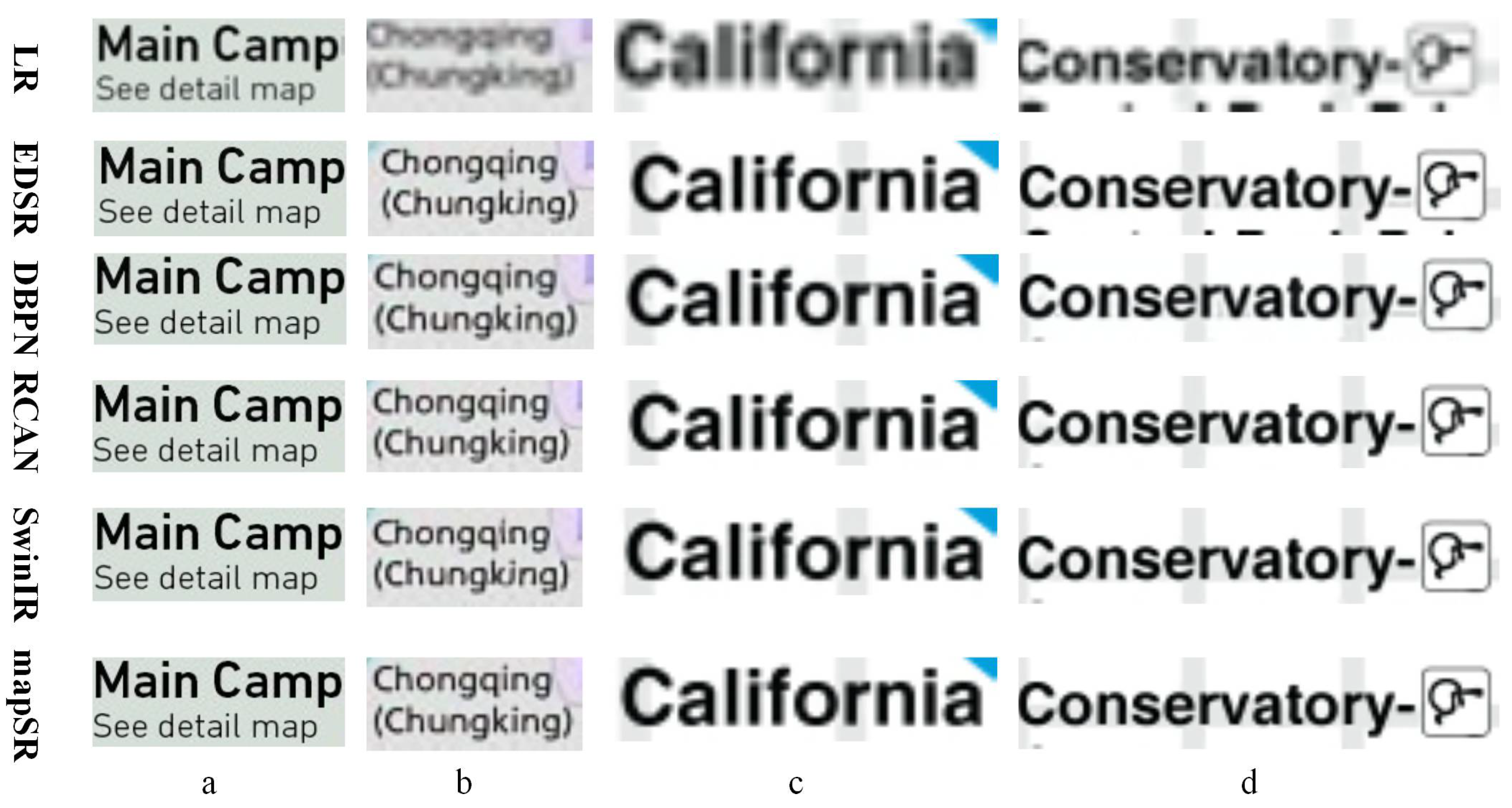
In addition, considering that text annotation is a key map feature to describe geospatial information, we also compared the results of text reconstruction from the low-resolution map. As shown in Figure 6 and Figure 7, our method was less noisy and clearer, especially for the reconstruction of words in all samples, which were unrecognizable in the original low-resolution map, and other methods had illegible details. Only our method achieved the best reconstruction and produced the best results.

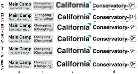
Figure 6. Results of map text reconstruction (2X). Subgraph (a–d) respectively denote the results of text reconstruction from four selected experimental groups.

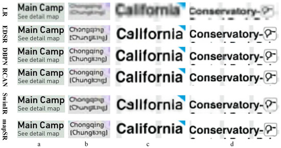
Figure 7. Results of map text reconstruction (3X). Subgraph (a–d) respectively denote the results of text reconstruction from four selected experimental groups.

4.2.3. Discussion

The differences between CNN- and ViT-based approaches are interesting. EDSR, DBPN, and RCAN were developed based on various CNN backbones, and SwinSR was developed based on the backbone of ViT. According to references in the community of pattern recognition [32,33], ViT-based deep learning approaches generally outperform CNN-based ones. However, the results shown in this manuscript were not similar. The results generated by SwinSR were never better than those generated by EDSR, DBPN, and RCAN. This was because there was much less well-labeled data in the raster maps. Since raster maps are considerably diverse in style, arrangement, background, etc., developing a benchmark dataset that holds large-scale information is still challenging. Moreover, ViT-based approaches always require much more computational load than CNN-based approaches, although both of these types of approaches are data-intensive computational tasks. Thus, when well-labeled raster map data are not available, CNN-based approaches are still an appropriate solution for map super-resolution.

Moreover, the differences between visual and quantitative evaluation are worthy of discussion. In the results of image super-resolution, the quantitative results generated by PNSR and SSIM were generally similar to the visual results. In this manuscript, we found that the results of these two evaluations were different to a degree. The task of image super-resolution mainly focuses on reconstruction regarding the authentic degree of visual recognition, including color, texture, etc. In the task of map super-resolution, the reconstruction of geospatial information (etc. map text characters) is also a critical concern, in addition to the degree of visual recognition. As shown in Figure 7, the text results generated by SwinSR were still difficult to visually recognize, although the quantitative evaluation deemed these results allowable.

5. Conclusions

Resolution is a critical factor in representing the content of a map. Low-resolution maps pose a big challenge for accurate text and symbol recognition, since the map text and symbols within them are not recognizable. Few previous investigations have focused on map feature recognition from low-resolution maps. This leads to a great number of low-resolution map resources being ignored.

In this paper, we proposed a novel model that fuses local and global features for the super-resolution reconstruction of low-resolution maps. Our proposed method modeled the global map features via the self-attention module and the local features by CNN modules. Then, we fused the global and local features to conduct map super-resolution reconstruction based on the overall map information and local map details. The experiment verified that our proposed method outperformed the state-of-the-art methods for map super-resolution reconstruction, and we also proved the effectiveness of the fusion of local and global features in improving the performance of map super-resolution.

In the future, several aspects might be worthy of attention. The optimization of LCB warrants exploration, since different LCB weights significantly affected the fusion of global and local features. In addition, besides extending the features derived from channel and spatial dimensions, the features generated from other aspects, such as Furious transform, might be useful for map super-resolution.

References

- Herold, M.; Liu, X.; Clarke, K.C. Spatial metrics and image texture for mapping urban land use. Photogramm. Eng. Remote Sens. 2003, 69, 991–1001. [Google Scholar] [CrossRef]
- Foo, P.; Warren, W.H.; Duchon, A.; Tarr, M.J. Do humans integrate routes into a cognitive map? Map- versus landmark-based navigation of novel shortcuts. J. Exp. Psychol. Learn. Mem. Cogn. 2005, 31, 195–215. [Google Scholar] [CrossRef] [PubMed]
- Qi, J.; Liu, H.; Liu, X.; Zhang, Y. Spatiotemporal evolution analysis of time-series land use change using self-organizing map to examine the zoning and scale effects. Comput. Environ. Urban 2019, 76, 11–23. [Google Scholar] [CrossRef]
- Sagl, G.; Delmelle, E.; Delmelle, E. Mapping collective human activity in an urban environment based on mobile phone data. Cartogr. Geogr. Inf. Sci. 2014, 41, 272–285. [Google Scholar] [CrossRef]
- Li, H.; Liu, J.; Zhou, X. Intelligent map reader: A framework for topographic map understanding with deep learning and gazetteer. IEEE Access 2018, 6, 25363–25376. [Google Scholar] [CrossRef]
- Pezeshk, A.; Tutwiler, R.L. Automatic feature extraction and text recognition from scanned topographic maps. IEEE Trans. Geosci. Remote Sens. 2011, 49, 5047–5063. [Google Scholar] [CrossRef]
- Leyk, S.; Boesch, R. Colors of the past: Color image segmentation in historical topographic maps based on homogeneity. Geoinformatica 2010, 14, 1–21. [Google Scholar] [CrossRef]
- Pouderoux, J.; Gonzato, J.; Pereira, A.; Guitton, P. Toponym recognition in scanned color topographic maps. In Proceedings of the Ninth International Conference on Document Analysis and Recognition, Curitiba, Brazil, 23–26 September 2007; Volume 1, IEEE. pp. 531–535. [Google Scholar]
- Zhou, X.; Li, W.; Arundel, S.T.; Liu, J. Deep convolutional neural networks for map-type classification. arXiv 2018, arXiv:1805.10402. [Google Scholar]
- Zhou, X. GeoAI-Enhanced Techniques to Support Geographical Knowledge Discovery from Big Geospatial Data; Arizona State University: Tempe, AZ, USA, 2019. [Google Scholar]
- Li, J.; Pei, Z.; Zeng, T. From beginner to master: A survey for deep learning-based single-image super-resolution. arXiv 2021, arXiv:2109.14335. [Google Scholar]
- Li, K.; Yang, S.; Dong, R.; Wang, X.; Huang, J. Survey of single image super-resolution reconstruction. IET Image Process. 2020, 14, 2273–2290. [Google Scholar] [CrossRef]
- Yang, Z.; Shi, P.; Pan, D. A Survey of Super-Resolution Based on Deep Learning. In Proceedings of the 2020 International Conference on Culture-Oriented Science & Technology, Beijing, China, 28–31 October 2020; pp. 514–518. [Google Scholar]
- Lu, Z.; Li, J.; Liu, H.; Huang, C.; Zhang, L.; Zeng, T. Transformer for single image super-resolution. In Proceedings of the IEEE/CVF Conference on Computer Vision and Pattern Recognition, New Orleans, LA, USA, 21–24 June 2022; pp. 457–466. [Google Scholar]
- Chen, X.; Wang, X.; Zhou, J.; Dong, C. Activating More Pixels in Image Super-Resolution Transformer. arXiv 2022, arXiv:2205.04437. [Google Scholar]
- LeCun, Y.; Bottou, L.; Bengio, Y.; Haffner, P. Gradient-based learning applied to document recognition. Proc. IEEE. 1998, 86, 2278–2324. [Google Scholar] [CrossRef]
- Dong, C.; Loy, C.C.; He, K.; Tang, X. Image super-resolution using deep convolutional networks. IEEE Trans. Pattern Anal. Mach. Intell. 2015, 38, 295–307. [Google Scholar] [CrossRef] [PubMed]
- Dong, C.; Loy, C.C.; Tang, X. Accelerating the super-resolution convolutional neural network. In Proceedings of the Computer Vision–ECCV 2016: 14th European Conference, Amsterdam, The Netherlands, 11–14 October 2016; pp. 391–407. [Google Scholar]
- Shi, W.; Caballero, J.; Huszár, F.; Totz, J.; Aitken, A.P.; Bishop, R.; Rueckert, D.; Wang, Z. Real-time single image and video super-resolution using an efficient sub-pixel convolutional neural network. In Proceedings of the IEEE Conference on Computer Vision and Pattern Recognition, Las Vegas, NV, USA, 27–30 June 2016; pp. 1874–1883. [Google Scholar]
- Kim, J.; Lee, J.K.; Lee, K.M. Accurate image super-resolution using very deep convolutional networks. In Proceedings of the IEEE Conference on Computer Vision and Pattern Recognition, Las Vegas, NV, USA, 27–30 June 2016; pp. 1646–1654. [Google Scholar]
- Kim, J.; Lee, J.K.; Lee, K.M. Deeply-recursive convolutional network for image super-resolution. In Proceedings of the IEEE Conference on Computer Vision and Pattern Recognition, Las Vegas, NV, USA, 27–30 June 2016; pp. 1637–1645. [Google Scholar]
- Lai, W.; Huang, J.; Ahuja, N.; Yang, M. Deep Laplacian pyramid networks for fast and accurate super-resolution. In Proceedings of the IEEE Conference on Computer Vision and Pattern Recognition, Honolulu, HI, USA, 21–26 July 2017; pp. 624–632. [Google Scholar]
- Lim, B.; Son, S.; Kim, H.; Nah, S.; Mu Lee, K. Enhanced deep residual networks for single image super-resolution. In Proceedings of the IEEE Conference on Computer Vision and Pattern Recognition Workshops, Honolulu, HI, USA, 21–26 July 2017; pp. 136–144. [Google Scholar]
- Haris, M.; Shakhnarovich, G.; Ukita, N. Deep back-projection networks for super-resolution. In Proceedings of the IEEE Conference on Computer Vision and Pattern Recognition, Salt Lake City, Utah, USA, 18–22 June 2018; pp. 1664–1673. [Google Scholar]
- Vaswani, A.; Shazeer, N.; Parmar, N.; Uszkoreit, J.; Jones, L.; Gomez, A.N.; Kaiser, A.; Polosukhin, I. Attention is all you need. Adv. Neural Inf. Process. Syst. 2017, 30, 5998–6008. [Google Scholar]
- Kaiser, L.; Bengio, S.; Roy, A.; Vaswani, A.; Parmar, N.; Uszkoreit, J.; Shazeer, N. Fast decoding in sequence models using discrete latent variables. In Proceedings of the International Conference on Machine Learning, Stockholm, Sweden, 10–15 July 2018; pp. 2390–2399. [Google Scholar]
- Dosovitskiy, A.; Beyer, L.; Kolesnikov, A.; Weissenborn, D.; Zhai, X.; Unterthiner, T.; Dehghani, M.; Minderer, M.; Heigold, G.; Gelly, S. An image is worth 16x16 words: Transformers for image recognition at scale. arXiv 2010, arXiv:2010.11929. [Google Scholar]
- Zhang, Y.; Li, K.; Li, K.; Wang, L.; Zhong, B.; Fu, Y. Image super-resolution using very deep residual channel attention networks. In Proceedings of the European Conference on Computer Vision, Munich, Germany, 8–14 September 2018; pp. 286–301. [Google Scholar]
- Dai, T.; Cai, J.; Zhang, Y.; Xia, S.; Zhang, L. Second-order attention network for single image super-resolution. In Proceedings of the IEEE/CVF Conference on Computer Vision and Pattern Recognition, Long Beach, CA, USA, 15–20 June 2019; pp. 11065–11074. [Google Scholar]
- Liang, J.; Cao, J.; Sun, G.; Zhang, K.; Van Gool, L.; Timofte, R. Swinir: Image restoration using swin transformer. In Proceedings of the IEEE/CVF International Conference on Computer Vision, Montreal, BC, Canada, 11–17 October 2021; pp. 1833–1844. [Google Scholar]
- Zhang, D.; Huang, F.; Liu, S.; Wang, X.; Jin, Z. SwinFIR: Revisiting the SWINIR with fast Fourier convolution and improved training for image super-resolution. arXiv 2022, arXiv:2208.11247. [Google Scholar]
- Han, K.; Wang, Y.; Chen, H.; Chen, X.; Guo, J.; Liu, Z.; Tang, Y.; Xiao, A.; Xu, C.; Xu, Y. A survey on vision transformer. IEEE Trans. Pattern Anal. Mach. Intell. 2022, 45, 87–110. [Google Scholar] [CrossRef]
- Shin, A.; Ishii, M.; Narihira, T. Perspectives and prospects on transformer architecture for cross-modal tasks with language and vision. Int. J. Comput. Vis. 2022, 130, 435–454. [Google Scholar] [CrossRef]
Disclaimer/Publisher’s Note: The statements, opinions and data contained in all publications are solely those of the individual author(s) and contributor(s) and not of MDPI and/or the editor(s). MDPI and/or the editor(s) disclaim responsibility for any injury to people or property resulting from any ideas, methods, instructions or products referred to in the content. |
© 2023 by the authors. Licensee MDPI, Basel, Switzerland. This article is an open access article distributed under the terms and conditions of the Creative Commons Attribution (CC BY) license (https://creativecommons.org/licenses/by/4.0/).