Quantifying the Effect of Socio-Economic Predictors and the Built Environment on Mental Health Events in Little Rock, AR

Abstract

Law enforcement agencies continue to grow in the use of spatial analysis to assist in identifying patterns of outcomes. Despite the critical nature of proper resource allocation for mental health incidents, there has been little progress in statistical modeling of the geo-spatial nature of mental health events in Little Rock, Arkansas. In this article, we provide insights into the spatial nature of mental health data from Little Rock, Arkansas between 2015 and 2018, under a supervised spatial modeling framework. We provide evidence of spatial clustering and identify the important features influencing such heterogeneity via a spatially informed hierarchy of generalized linear, tree-based, and spatial regression models, viz. the Poisson regression model, the random forest model, the spatial Durbin error model, and the Manski model. The insights obtained from these different models are presented here along with their relative predictive performances. The inferential tools developed here can be used in a broad variety of spatial modeling contexts and have the potential to aid both law enforcement agencies and the city in properly allocating resources. We were able to identify several built-environment and socio-demographic measures related to mental health calls while noting that the results indicated that there are unmeasured factors that contribute to the number of events.

1. Introduction

Over the past two decades, law enforcement agencies are relying more and more on statistical tools to build an objective criminal justice system, leading to a meteoric rise in “predictive policing”, loosely defined as “the application of analytical techniques—particularly quantitative techniques—to identify likely targets for police intervention and prevent crime or solve past crimes by making statistical predictions” [1]. Research has continued to point to crime not occurring randomly in space, leading to the Law of Crime Concentration [2,3] and the Fact of Hotspots [4]. This has been met with interest by the U.S. National Institute of Justice’s Real Time Crime Forecasting Challenge [5] that was designed to identify accurate and efficient approaches to crime forecasting.

Apart from increasing the accuracy of prediction of future law enforcement-related events (e.g., crime and calls for service), it is also important to understand which geographical factors significantly contribute to these calls for service. Such knowledge can inform a plan for allocating resources or making policy changes to either counteract the effect of a “risky” place or increase the intensity or presence of a “protective” place. Given that the knowledge gained from predictive models can inform both the allocation of resources and policy change, it is imperative to ensure that any prediction rule does not suffer from algorithmic or systemic biases. This is particularly important, as with the increase in complexity and use of such data-based tools, there is growing concern about and additional effort devoted to reducing racial disparities in predictive policing, while still producing dynamic and real-time forecasts and insights about spatio-temporal crime activities. For example, using a combination of demographically representative synthetic data and survey data on drug use, it was found that predictive policing estimates based on biased policing records often accentuate racial bias instead of removing it [6].

In the field of criminal justice and criminology, the spatial distribution of events is often linked to two theoretical fields: communities and crime [7,8,9], and crime and place [2,10]. At a larger spatial unit, the communities and crime theoretical field typically uses Census tracts and block groups as boundaries to integrate social measures. This level of analysis is often joined with a Social Disorganization theoretical framework [8]. In short, crime occurs disproportionately more frequently in communities described as disadvantaged (e.g., poverty, unemployment, education, median household income, amongst others). This literature has continued to support the idea that community context matters and community disadvantage remains a robust predictor of community levels of crime [11].

Moving to a more micro-level (e.g., points, grid cell, street segment) spatial approach to understanding crime occurrence, the crime and place research uses Routine Activities Theory [12] and Crime Pattern Theory [13]. Here, crime occurrence is influenced by people’s general daily activities as people develop a greater awareness when traveling to their common activity spaces, identifying potential crime opportunities (or being identified as a potential target). Furthermore, as individuals engage in their routine activities, they may inadvertently frequent or inhabit proximate locations known to criminologists as crime generators or attractors [14]. Crime generators/attractors are places known to elevate crime occurrence and some more common types studied are bars [15,16], public transit [17,18], and parks [19,20], while a growing body of literature examines multiple types of crime generators/attractors on their overall ability to predict crime occurrence [21,22]. For instance, the co-location of multiple factors of the built environment that create future risk, such as public transit in close proximity to a bar, would result in greater risk.

Together, the two theoretical fields suggest that both communities and place provide an outline for what factors contribute to crime occurrence in space; however, it is important to highlight that not all crime has similar spatial distributions. Broader spatial criminology has indicated the need to disaggregate crime types to better understand the spatial distribution of specific crime types [23]. That is, depending on the specific crime type or call-for-service, the spatial distributions could be entirely different from one another. For instance, residential and commercial burglary are different crime types; although both are still burglary, they have different target availabilities (i.e., house versus business).

Moreover, police are often called for services that are not necessarily criminal, and the spatial distribution of these calls for service might vastly differ from those calls associated with other crime types. Police are utilized for all different types of services beyond responding to crime (e.g., person checks, directions, house checks, vehicle crashes). Because of this, there needs to be greater attention paid to call-type disaggregation to better understand policing services overall. In particular, police response to mental health-related calls has drawn greater attention in recent years [24,25,26,27,28,29,30]. Vaughan et al. [29] found temporal patterns with mental health-related calls for service, finding that certain months of the year and days of the week generated greater call volume. Moving from temporal to spatial, Hodgkinson and Andresen [24] found that approximately 14% of policing calls for service are related to mental health, while violence accounted for only about 2%, and these calls tended to cluster around social service locations (e.g., people without housing and shelter). Spatial findings continue to support that there might exist a clustering of mental health-related calls for service. Identification of spatial clustering of mental health-related calls for service is an important step in analysis as it would follow general patterns of other crimes; however, there is a limitation in that we need to identify what contributes to the clustering of these mental health-related calls for service.

The current study seeks to overcome this gap by building on limited research [27] to identify characteristics of the built and social environment that influence mental health calls for service. To better understand the spatial distribution of mental health calls for service, the current study employs multiple techniques. The proposed algorithms and methods attempt to uncover and exploit different aspects of policing calls for service. For example, Gotway and Stroup [31] used a spatial generalized linear model that had been extended both by considering the temporal pattern and by a non-linear modeling approach using generalized additive modeling [32].

Our focus is on understanding the spatial characteristics of mental health-related calls for service. This includes starting from a general cluster analysis to modeling to identify significant predictors for mental health calls for service. Furthermore, this article adds to the extant literature on leveraging interpretable statistical and machine learning tools to identify important predictors that either improve the predictive accuracy or explain unobserved variability in crime data, see e.g., Wheeler and Steenbeek [33]. We briefly introduce the study area, data aggregation and the methodology in Section 2, compare model performances in Section 3, and conclude with a discussion in Section 4.

2. Materials and Methods

2.1. Study Area

In this study, we focus on the capital city Little Rock, Arkansas, to understand the spatial occurrence of mental health-related calls for service. Little Rock regularly has above-average violent and property crime rates when compared to other large U.S. cities. Additionally, Little Rock has a long history of segregation [34] creating spatially distinct areas of the city. Overall, Little Rock is about 120 square miles with a population of just over 200,000 people. Little Rock is the largest city in Arkansas, doubling the next largest city, Fayetteville.

2.2. Data & Pre-Processing

Data were obtained from several city departments, including the Little Rock Police Department (LRPD), through an ongoing data-sharing Memorandum of Understanding (MOU) between researchers and Little Rock. Social data were obtained from the American Community Survey (5-year estimates). Mental health incidents from 2015 through 2017 were used to predict 2018 incidents.

The data used in the current study were compiled from twenty-nine constituent geospatial data sets that include crime incidents, sociodemographic variables, and individual landmarks (such as police stations or rental apartments). These datasets were spatially joined together to create a comprehensive master data set for subsequent analysis. We evaluated potential risk and protective factors in terms of four criteria. These criteria included accessibility, geographic scale, temporal scale, and inclusion in the literature as risk factors for mental health incidents or spatial attractors of risk factors for mental health incidents. Key population metrics were also included. See

Table 1. Independent Variables (Abbreviations used: ACS: American Community Survey, LRPD: Little Rock Police Department, LRSD: Little Rock School District.).

Potential Community Protective Factors X-Y Coordinates	Source
Banks	Little Rock City
Childcare Services	InfoGroup
Child/Youth Services	InfoGroup
Civic/Social Organizations	InfoGroup
Grocery Stores	Little Rock City
High Schools (Public)	LRSD Website
Hospitals	InfoGroup
Neighborhood Resource Centers	Little Rock City
Police/Fire Facilities	Little Rock City
Religious Organizations	InfoGroup
Potential Community Risk Factors X-Y coordinates	Source
Barber and Beauty Shops	Little Rock City
Bus Stops	MetroPlan
Check Cashing and Pawn Shops	Little Rock City
Fast-Food and Beverage Restaurants	Little Rock City
Gas Stations and Convenience Stores	Little Rock City
Hotels and Motels	Little Rock City
Liquor Stores	AR Alcohol Beverage Control
Major Dept. Discount Stores	Little Rock City
Mixed Drink-Bar, Restaurants, and Clubs	AR Alcohol Beverage Control
Rental Mobile Homes	Little Rock City
Rental Single to Quad	Little Rock City
Rental Apartments < 100 units	Little Rock City
Rental Apartments > 100 units	Little Rock City
Tattoo Piercing	Little Rock City
Unsafe and Vacant Buildings	Little Rock City
Crime (Antisocial behavior of community) X-Y coordinates	Source
Agg. Assault: Household Member	LRPD
Agg. Assault	LRPD
Battery: 1st degree	LRPD
Battery: 2nd Degree	LRPD
Breaking or Entering Vehicle	LRPD
Burglary: Residential	LRPD
Burglary: Commercial	LRPD
Domestic Battering	LRPD
Drugs Narcotics	LRPD
Rape	LRPD
Robbery	LRPD
Robbery (Aggravated)	LRPD
Runaways	LRPD
Terroristic Act	LRPD
Theft of Property: Misdemeanor	LRPD
Theft of Property: Felony	LRPD
Population Metrics extrapolated from census track data	Source
Population Density	ACS
Percent Black	ACS
Percent Non-White	ACS
Percent Hispanic	ACS
Percent Under 18	ACS
Percent College Educated	ACS
Percent Less than High School Degree	ACS
Percent in Poverty (under 18)	ACS
Percent Population Struggling	ACS
Percent Single Parent Households	ACS
Percent Female Headed Households	ACS
Percent Non-Married Households	ACS
Percent on Public Insurance	ACS
Percent Not Insured	ACS
Percent Home Ownership	ACS
Percent Renter Occupied Households	ACS

for a complete list of independent variables used in this study.

We created a lattice grid of polygons to standardize the location of individual mental health events and contributing factors, without conforming to predefined political or social boundaries. The appropriate grid cell size was determined by examining the distribution of the count of mental health events at various grid cell sizes. A 1000 by 1000-foot square grid size was chosen to cover the study area and minimize blank spaces from areas without population. The optimal grid size was chosen using the Bayesian Information Criterion (BIC) to check goodness of fit for Poisson distribution for mental health incident counts in each cell. The optimal cell size is the elbow point of the resulting goodness-of-fit plot, which is approximately five city blocks and amenable to targeted community interventions on a smaller spatial scale compared to neighborhoods. Each grid cell was assigned to its corresponding census tract using cell centroids. Raw count data for screened-in mental health reports were aggregated to grid cells, and the report rate per 100 people was calculated by interpolating 2010 US Census population data to each grid cell, then normalized to a zero-to-one scale.

We utilized the open-source programming language and software R Version 3.6.2 [35] for all data manipulations and statistical models. R provides unparalleled opportunities for analyzing spatial data for spatial modeling, which was crucial for our analysis. We employed a supervised learning approach to predict and infer spatial risk factors for mental health using established raster data models [36]. We calculated counts of mental health and standard social and environmental factors for each grid cell and used them as the foundation for our supervised learning model. We examined various models, including the Poisson generalized linear model, the spatial Durbin and Manski models, and non-linear tree-based methods (random forest model), to inform aspects of the spatial process and learning assessment, based on distributional assumptions and criteria and informed by exploratory analyses.

2.3. Methods

2.3.1. Poisson Generalized Linear Model

The Poisson regression model belongs to a family of regression models called the generalized linear model (GLM). As a special case of the GLM family, the fitted Poisson regression model uses $\mathsf{\eta }=\mathrm{l}\mathrm{o}\mathrm{g}\left(\mathsf{\lambda }\right)$ as a canonical link and is of the form:

$$\widehat{{\mathrm{y}}_{\mathrm{i}}}=\widehat{\mathrm{E}\left({\mathrm{y}}_{\mathrm{i}}\right|{\mathrm{x}}_{\mathrm{i}})}={\mathrm{g}}^{-1}\left({\mathrm{x}}_{\mathrm{i}}^{\mathrm{T}} \widehat{\mathsf{\beta }}\right)={\mathrm{e}}^{{\mathrm{x}}_{\mathrm{i}}^{\mathrm{T}} \widehat{\mathsf{\beta }}}$$

Among several link functions commonly used with the Poisson distribution, the log link function ensures that ${\mathsf{\lambda }}_{\mathrm{i}}\ge 0$, which is crucial for the expected value of a count outcome of the response variable, e.g., mental health incidents [37], given the predictor variables will be non-negative. In terms of model interpretation, parameters may be interpreted in a probabilistic sense, which arises as an advantage from the fact that Poisson regression belongs to the GLM family. Consequently, significant factors present in the fitted model may be explained in strict probabilistic terms with respective levels of uncertainty.

2.3.2. Random Forest

Random forest falls into the non-linear/non-parametric category of supervised learning approaches known as decision trees [38]. Decision trees are particularly well known due to their inherent ease of use and interpretability in both regression and classification problems. For regression problems, which we focus on here, decision trees divide the predictor space into J distinct and non-overlapping regions, ${\mathrm{R}}_1,{\mathrm{R}}_2,\dots ,{\mathrm{R}}_{\mathrm{J}=\left|\mathrm{T}\right|}$ also known as terminal nodes or leaves using the training data through a recursive binary splitting procedure. Note that a threshold is implemented so that the recursive binary splitting procedure ends when the number of observations at any terminal node falls below the set threshold. In addition to the preceding criteria, the aim is to obtain terminal nodes that minimize the residual sum of squares:

$${\displaystyle \sum _{\mathrm{j}=1}^{\left|\mathrm{T}\right|}}\sum _{\mathrm{i}\in {\mathrm{R}}_{\mathrm{j}}}{\left({\mathrm{y}}_{\mathrm{i}}-{\mathrm{y}}_{{\mathrm{R}}_{\mathrm{j}}}\right)}^2$$

The results obtained are likely to over-fit the data due to the complexity of the resulting tree, so a cost–complexity pruning procedure is implemented to find a sub-tree which minimizes the objective function:

$${\displaystyle \sum _{\mathrm{j}=1}^{\left|\mathrm{T}\right|}}\sum _{\mathrm{i}\in {\mathrm{R}}_{\mathrm{j}}}{\left({\mathrm{y}}_{\mathrm{i}}-{\mathrm{y}}_{{\mathrm{R}}_{\mathrm{j}}}\right)}^2+\mathsf{\alpha }\left|\mathrm{T}\right|,$$

where the $\mathsf{\alpha }\left|\mathrm{T}\right|$ term is a model–complexity penalty with $\left|\mathrm{T}\right|$ denoting the number of terminal nodes and degree of penalization determined by the tuning parameter $\mathsf{\alpha }$. This extra penalty term reduces the variance at the cost of little bias for better interpretation. The predicted response for any observation that falls into the ${\mathrm{R}}_{\mathrm{i}}^{\mathrm{t}\mathrm{h}}$ region is the mean response of all observations from the training data set that are in that same terminal node.

Single decision trees, however, are not as competitive when compared to other forms of linear or non-linear supervised learning models. One solution to building a more robust decision tree is known as random forests. Random forests build many decision trees to improve performance using bootstrapped samples from the training data and using only a subset of available predictors in the tree-building stages, a process that decorrelates the trees. The final prediction is then accomplished by averaging the predictions from each of the individual trees, or by majority voting, depending on the task at hand. Specifically, in the process of building each decision tree, at every stage or split, a random sample of size m = √p predictors are chosen as candidates from the pool of p predictors. As a result, strong predictors do not influence the building order of every tree (making them dissimilar). This process decorrelates the many trees, as on average (p–m)/p of the splits would not have such strong predictors, thus reducing the variance and improving results via bias–variance tradeoff. We refer the reader to James et al. [39] for an in-depth discussion of random forests. In relation to crime, Wheeler and Steenbeek [33] found their random forests model outperformed RTM and Kernel Density Estimations (KDE) for robbery prediction in Dallas, Texas.

2.3.3. Spatial Econometric Models

Data containing a location/geographic component contain spatial dependencies among observations which may lead to spatial relationships. Spatial relationships occur not only in the dependent variables (response variables) but also in the independent variables (covariates) and residual terms (ϵ). The proper terms defining spatial relationships among dependent variables, independent variables, and residual terms are known as endogenous interaction, exogenous interaction, and error interaction, respectively. According to Elhorst [40], a model that accounts for all spatial relationships is the Manski model (also known as the Generalized Nesting Spatial Model, GNS), with the form:

$$\mathrm{Y}=\mathsf{\delta }\mathrm{W}\mathrm{Y}+\mathrm{X}\mathsf{\beta }+\mathrm{W}\mathrm{X}\mathsf{\theta }+\mathrm{u}; \mathrm{u}=\mathsf{\lambda }\mathrm{W}\mathrm{u}+\mathsf{ϵ}$$

Here $\mathsf{\delta }$ is known as the spatial autoregressive coefficient, $\mathsf{\lambda }$ is the spatial autocorrelation coefficient, $\mathrm{W}$ represents the spatial weights matrix that describes the spatial configuration of the unit samples, $\mathrm{X}$ is a matrix of exogenous variables or covariates and lastly $\mathsf{\theta }$ and $\mathsf{\beta }$ are unknown parameters to be estimated that explain the contribution of each predictor and their spatially lagged version [40].

For the purpose of this study, both the Manski model and the SDEM were fitted onto the mental health spatial data. The Manski model (otherwise known as GNS) models spatial events, e.g., mental health incidents, as a function of endogenous interactions (neighboring values or spatial lags), exogenous interactions (built environment, social factors, etc.), and error interactions (spatial autocorrelation and spatial heterogeneity). The SDEM is a special case of a Manski model with $\mathsf{\delta }=0$, thus having the endogenous interactions removed. The SDEM is of the form:

$$\mathrm{Y}=\mathrm{X}\mathsf{\beta }+\mathrm{W}\mathrm{X}\mathsf{\theta }+\mathrm{u}; \mathrm{u}=\mathsf{\lambda }\mathrm{W}\mathrm{u}+\mathsf{ϵ}$$

3. Results

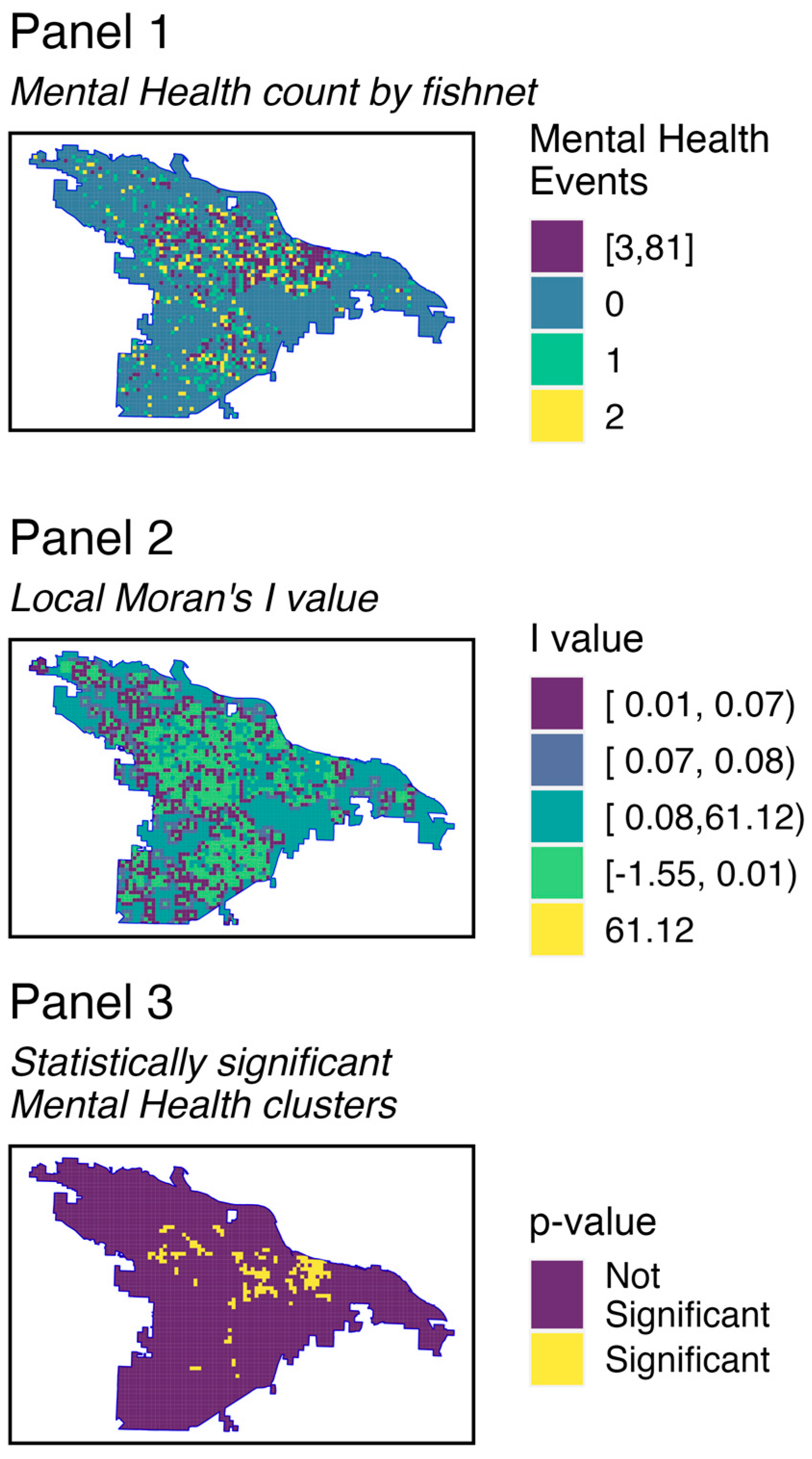
3.1. Evidence of Spatial Clustering

The underlying assumption at the start of this study was that mental health incident events in Little Rock were distributed as spatially heterogeneous points (i.e., clusters) rather than uniformly over the geographic region. To put matters into visual perspective, see Figure 1, where panel 1 represents the geographic locations of the recorded 2018 mental health incidents in Little Rock and panel 2 represents the same number of incidents but simulated as if they were following a uniform spatial distribution without any spatial clustering. Figure 1 shows the presence of spatial clusters of mental health incidents in Little Rock when compared with the uniform distribution. However, as visual comparisons could be interpreted as being subjective, we consider a measure of spatial auto-correlation to test the spatial heterogeneity. To be precise, we want to test the null hypothesis that the mental health incidents are uniformly distributed across the area of study (Little Rock) against the alternative hypothesis that they are more clustered than might be expected from usual randomness.

Clustering, when referring to the whole spatial pattern, can be described by a global statistic for spatial auto-correlation. However, to properly identify the location of clustered and non-clustered regions, a Local Indicator of Spatial Association (LISA) must be implemented. A LISA is any statistic that provides the extent of significant spatial clustering of similar values around a given observation (i.e., a Local Spatial Statistic). It also establishes the connection between the local and global statistic for spatial association as being that the sum of all local spatial statistics is proportional to the global statistic, thereby allowing for the decomposition of global indicators [41].

Among a number of global tests for spatial auto-correlation, including Geary’s C and the global Getis-G, Moran’s I is perhaps the most common global test and is implemented in almost all common spatial toolboxes for testing auto-correlation [42]. Spatial auto-correlation quantifies the degree to which similar features cluster and identifies their location. In the presence of spatial auto-correlation, we can predict the values of observation i from the values observed at $j\in N_i$, the set of its proximate neighbors [43]. As in typical correlation, Moran’s I value generally ranges from −1 to +1 inclusively as a result of having a normalizing factor [44]. The contrast between spatial auto-correlation Moran’s I and Pearson’s or Spearman’s correlation lies in the presence of the spatial weights matrix in Moran’s I statistic. The inclusion of the spatial weights matrix in Moran’s I enables the possibility of obtaining extreme values greater than the usual (−1, 1) bounds depending on the structure and composition of the weights matrix. Extreme values are obtained via the relation between the minimum and maximum eigenvalues from the spatial weights matrix. For a thorough discussion regarding the range and extreme values of Moran’s I we refer readers to [45]. A negative and significant Moran’s I value represents negative spatial auto-correlation, indicating that dissimilar values are next to each other. A positive and significant Moran’s I value represents positive spatial auto-correlation, indicating evidence of clustering of like values.

$$\frac{\mathrm{n}}{{\sum }_{\mathrm{i}=1}^{\mathrm{n}}{\sum }_{\mathrm{j}=1}^{\mathrm{n}}{\mathrm{w}}_{\mathrm{i}\mathrm{j}}}$$

In order to apply the spatial auto-correlation tests (both Global and Local Moran’s I) onto the spatial data and induce a supervised learning framework, two critical prerequisite steps had to be executed, viz. (a) identification of the k-nearest neighbors, and (b) assigning their respective weights using the package spdep [46]. We used the incident counts by the fishnet of grid cell size of 1000 ft by 1000 ft from Little Rock containing all the necessary attributes for the analysis, with each cell mapped to a centroid, which was necessary in order to extend the neighborhood criteria from contiguity to distance-based neighbors (i.e., k-nearest neighbors) [42]. Grid cell is a common spatial unit of analysis used in criminological research [22].

Using k-nearest neighbors typically leads to asymmetric neighbors. However, this is not the case here as all centroids are uniformly spaced. A key advantage of using distance-based neighbors to ordinary polygon contiguity is that it ensures that all fishnet grid cells’ polygon representation (centroids) have k neighbors. It is common practice to use k = 8 or k = 4 neighbors, which are formally known as “Queen case” and “Rook case”. For this study, k = 8 nearest neighbors were used and located using the function knearneigh and Knn2nb from the spdep package. Following the identification of the eight nearest neighbors for each centroid, their respective weights were assigned using the function nb2listw from the same spdep package. In this current work, we assigned equal weights to each grid cell’s nearest neighbors, implying that each neighbor would have a corresponding weight of 1/8, which was then used to compute the mean neighbor values, i.e., $weigh{t}_i=\frac{1}{8}{\sum }_{i=2}^{9}neighbo{r}_i$. This was equivalent to averaging over all mental health incident cases occurring within the eight neighbor grid cells. Having obtained both the neighbors and their respective weights, we tested for the presence of spatial auto-correlation using both Global Moran’s I and Local Moran’s I, as seen in Figure 2.

3.2. Model Comparison

We compared the predictive performance of the four candidate methods in

Table 2. Model Performance Comparison. (NA: Not Applicable, as standard errors were calculated via a spatial cross-validation and were not feasible for the spatial econometrics models.)

Model	MAPE Mean (SD)	MAE Mean (SD)	RMSE Mean (SD)
Poisson GLM	1.311 (0.031)	0.910 (0.270)	2.917 (1.589)
Random Forest	1.306 (0.035)	0.868 (0.171)	2.190 (0.901)
Spatial Durbin	1.316 (NA)	0.636 (NA)	2.135 (NA)
Manski Model	1.302 (NA)	0.771 (NA)	2.583 (NA)

and report the mean and standard deviation for each error measure. To better assess the accuracy of the models, we used four different error measures: Mean Absolute Percentage Error (MAPE), Mean Absolute Error (MAE) and Root Mean Square Error (RMSE), see Table 2. The errors were calculated in a supervised learning set-up, where both the Poisson regression and the random forest models were built using fivefold cross-validation for tuning parameters.

Below, we define the different error measures used to compare and describe the best performing model according to that criterion. First, the Mean Absolute Percentage Error (MAPE) statistic captures the model’s accuracy in terms of percentage error. The MAPE is calculated using the following formula:

$$\mathrm{M}\mathrm{A}\mathrm{P}\mathrm{E}=\frac{1}{\mathrm{n}}{\displaystyle \sum _{\mathrm{i}=1}^{\mathrm{n}}}\left|\frac{{\mathrm{A}}_{\mathrm{i}}-{\mathrm{F}}_{\mathrm{i}}}{{\mathrm{A}}_{\mathrm{i}}}\right|\times 100,$$

where ${\mathrm{A}}_{\mathrm{i}}$ is the ith actual observation and ${\mathrm{F}}_{\mathrm{i}}$ is the ith forecast value. Since the MAPE expresses the error as a percentage, it can be relatively easier to interpret when compared to other statistic measures. The lower the percentage error, the more accurate the model represents the data. For a given model, it can be concluded that on average, the forecast is off by the MAPE % age amount. In this case, on average all the models’ forecasts were off by approximately 1.3% with a standard deviation of approximately 0.0308 and 0.0346 for the Poisson GLM and random forest models, respectively. In terms of MAPE, all the models performed relatively the same, with the Manski model having the smallest MAPE.

The Mean Absolute Error (MAE) statistic, given by the formula $\mathrm{M}\mathrm{A}\mathrm{E}=\frac{1}{\mathrm{n}}{\sum }_{\mathrm{i}=1}^{\mathrm{n}}\left|{\mathrm{A}}_{\mathrm{i}}-{\mathrm{F}}_{\mathrm{i}}\right|$, where ${\mathrm{A}}_{\mathrm{i}}$ is the ith actual observation and ${\mathrm{F}}_{\mathrm{i}}$ is the ith forecast value, captures on average how large the forecast error is expected to be. The spatial Durbin error model had on average the smallest forecast error of 0.6356, followed by the Manski model with a MAE of 0.7708, and the Poisson GLM had the largest forecast error of 0.9098. Finally, the Root Mean Square Error (RMSE), given by $\frac{\sqrt{{\left({\mathrm{A}}_{\mathrm{i}}-{\mathrm{F}}_{\mathrm{i}}\right)}^2}}{\mathrm{n}},$ calculates the square root of the average of the square errors. The RMSE measures the spread of the prediction errors. The spatial Durbin error model had the smallest RMSE value of 2.135, followed by the random forest model with an RMSE of 2.1904, and the Poisson GLM had the largest RMSE of 2.9166.

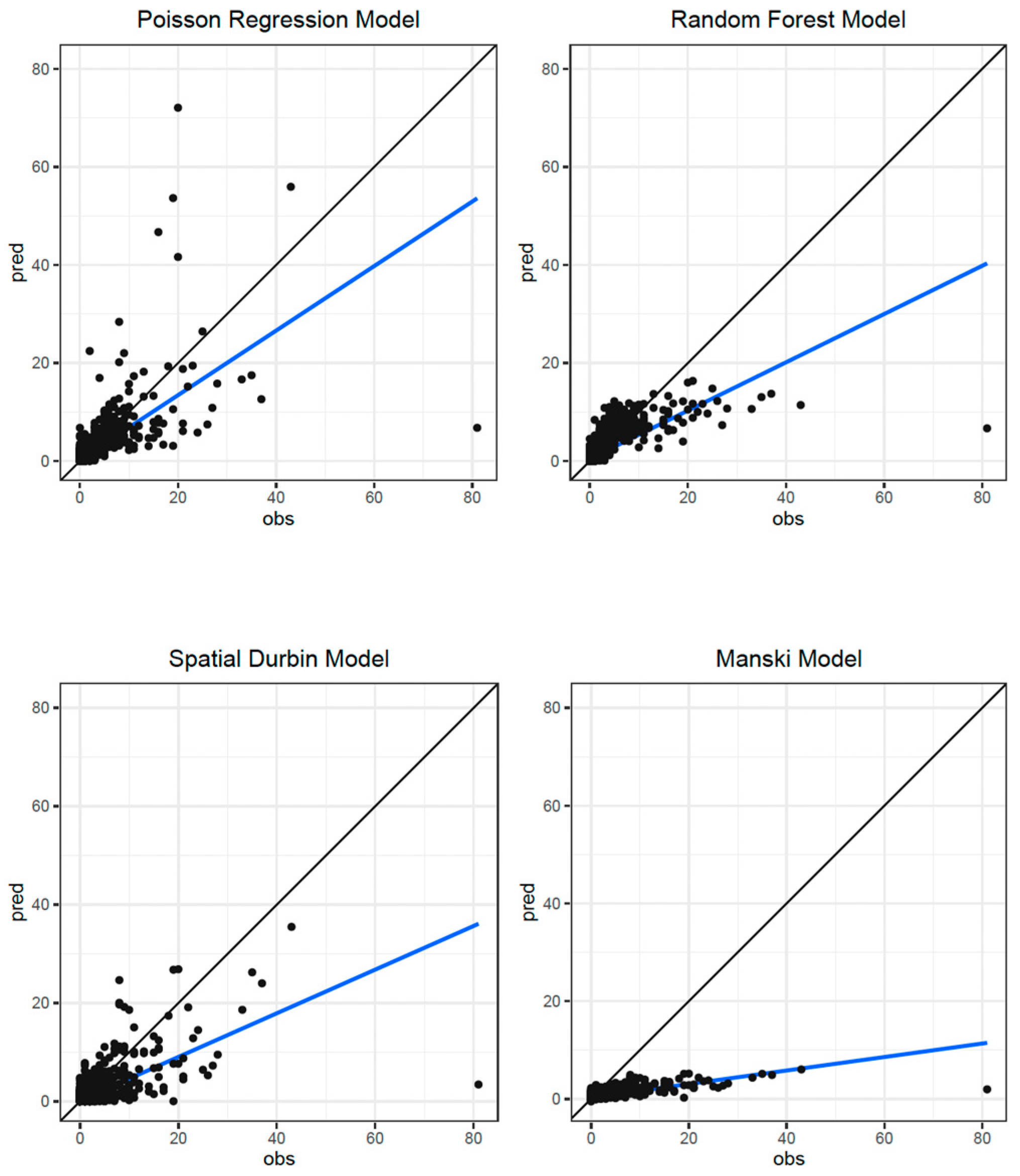
3.2.1. Model Performance

In terms of goodness-of-fit metrics, the R squared ($R^2$) values and logarithmic deviance score were used to evaluate the models. The most common measure is perhaps the $R^2$ that represents the percentage of variation explained by the model,

$$R^2=1-\frac{\sum {\left(y_i-\widehat{y_i}\right)}^2}{\sum {(y_i-\stackrel{-}{y})}^2}.$$

Thus, a larger $R^2$ is indicative of a better model fit. Note that we did not report the adjusted $R^2$ values (or similar criteria that account for model dimension) as they are rather difficult to compute for distribution-free models such as random forest and, thus, difficult to use in the goodness-of-fit comparison between our current models. The Logarithmic Deviance score is a measure of the deviance between the predicted and observed counts, via the log likelihood ratio. To measure this, we calculated the likelihood ratio of the observed value and the predicted value based on a Poisson distribution. The goodness of fit reported here is the negative log of the probability density, so a lower value indicates a better predictive ability. As seen in

Table 3. Model Goodness-of-Fit Comparison. (NA: Not Applicable, as standard errors were calculated via a spatial cross-validation and were not feasible for the spatial econometrics models.)

Model	R2 Mean (SD)	Log Deviance Mean (SD)
Poisson GLM	0.393 (0.152)	0.614 (0.051)
Random Forest	0.382 (0.058)	0.584 (0.040)
Spatial Durbin	0.474 (NA)	0.710 (NA)
Manski Model	0.437 (NA)	0.612 (NA)

and Figure 3, the spatial Durbin error model obtained the largest R square value, followed by the Manski model. Note that despite having obtained the largest R square value, i.e., the best model in terms of R square goodness-of-fit metric, the spatial Durbin error model obtained the largest logarithmic deviance score and was thus the worst model in terms of the logarithmic deviance score goodness-of-fit metric for the mental health data. In terms of the logarithmic deviance score goodness-of-fit metric, the random forest model obtained the smallest score. This suggests that the random forest model had the smallest deviance between predicted and observed count of mental health incidents, i.e., it was the best model of that category.

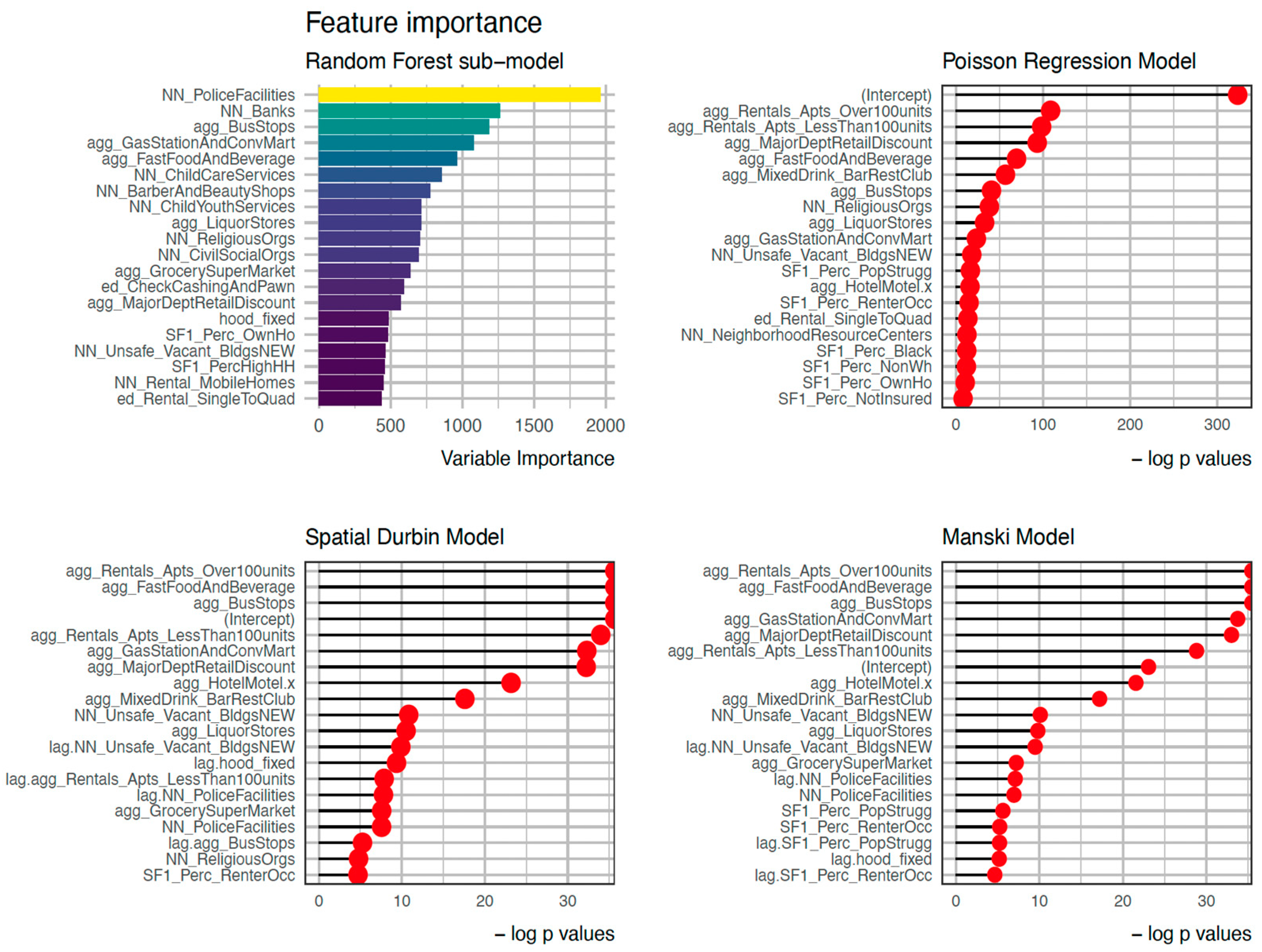
3.2.2. Feature Importance

Finally, we look at the important features or variables driving the prediction for each of the four candidate methods. We call these measures “variable importance” following the nomenclature used by random forest literature, but for purely statistical models such as the Poisson regression or spatial Durbin models, the quantities being compared are a measure of each variable’s significance. As discussed before, this a key step in the prediction process, as the identification of important variables help us in determining which environmental and social features are predominantly occupying each of these predictive processes, investigate whether they play a risky or protective role, and then allocate resources accordingly.

A note about nomenclature for the features plotted on the following figures: there are three unique prefixes linked with each type of feature. Nearest neighbor (“NN”) refers to features obtained by calculating the average distance between a fishnet grid cell centroid and its nearest neighbor in the Queen case definition. Euclidean distance (“ed”) refers to features obtained by calculating the Euclidean distance between a fishnet grid cell centroid and its first nearest neighbor. The prefix “agg” refers to the count of mental health incidents in a given fishnet grid cell. The term “agg” was coined based on the aggregate function used in R to obtain the count of cases associated per fishnet cell.

Table 4. Variable importance across models.

Poisson GLM	Random Forest	Spatial Durbin	Manski
agg Rentals Apts Over100 units	NN PoliceFacilities	agg Rentals Apts Over100 units	agg Rentals Apts Over100 units
agg Rentals Apts LessThan100 units	NN Banks	agg FastFoodAndBeverage	agg FastFoodAndBeverage
agg MajorDeptRetailDiscount	agg BusStops	agg BusStops	agg BusStops
agg FastFoodAndBeverage	agg GasStationAndConvMart	agg Rentals Apts LessThan100 units	agg GasStationAndConvMart
agg MixedDrink BarRestClub	agg FastFoodAndBeverage	agg GasStationAndConvMart	agg MajorDeptRetailDiscount
agg BusStops	NN ChildCareServices	agg MajorDeptRetailDiscount	agg Rentals Apts LessThan100 units
NN ReligiousOrgs	NN BarberAndBeautyShops	agg HotelMotel.x	agg HotelMotel.x
agg LiquorStores	NN ChildYouthServices	agg MixedDrink BarRestClub	agg MixedDrink BarRestClub
agg GasStationAndConvMart	agg LiquorStores	NN Unsafe Vacant BldgsNEW	NN Unsafe Vacant BldgsNEW
NN Unsafe Vacant BldgsNEW	NN ReligiousOrgs	agg LiquorStores	agg LiquorStores

summarizes the top ten most influential features from each model. We note here that four similar features were found among the set of top features selected for each of the four models. These common spatial features were: fast food and beverage places, bus stops, liquor stores, gas stations, and convenience marts. As the four models highlight the importance of the influence these features had on the models, further interdisciplinary study involving experts from criminology and local law enforcement is required to understand whether any causal relationship exists between these environmental factors and mental health incidents in Little Rock, Arkansas.

Figure 4 illustrates the feature importance in descending order with respect to each model. In order to create a visual feature comparison between the random forest model feature importance and the remaining models, the $-{\mathit{log}}_{10}P$-values of each predictor were plotted for the other three models.

4. Discussion

In this study, we used a supervised machine learning framework to understand the effect of sociodemographic as well as environmental factors in predicting the spatial clusters of mental health incidents in Little Rock, Arkansas. The use of Moran’s I for exploratory data analysis of existent spatial auto-correlation revealed an uneven distribution of mental health incidents across the area of study. We compared four different statistical methods, judiciously chosen to cover a diverse array of parametric, non-parametric, linear, and non-linear methods, in terms of their prediction accuracy and goodness of fit. The order of important factors (see Figure 4) provides insight into the spatial and sociodemographic factors associated with the spatial distribution of mental health incidents in Little Rock, Arkansas. We note here that these associations are not causal in nature and many of them are endogenous, rather than exogenous, and caution must be exercised when interpreting these results in terms of broader policy evaluations.

The metrics of performance indicate that in terms of prediction accuracy, the spatial econometric models (Manski model and spatial Durbin error model) performed slightly better than their model counterparts, which is most likely indicative of the importance of fitting explicit spatial factors into the former models. For the model goodness of fit based upon R-squared and logarithmic deviance score, respectively, the spatial Durbin error model and random forest model performed the best, although the maximum of these values was still low, e.g., highest R² ~ 0.474 (Durbin), suggesting the presence of some variability in the data not explained by any of these models. The incorporation of these models would allow for law enforcement agencies to better allocate resources and address the unequal distribution of these mental health-related calls for service.

Furthermore, if law enforcement agencies adopt this framework, a meta model created from the models generated may serve as a better tool, if there is indecision regarding which model to select based on prediction accuracy or goodness of fit. In addition to creating a meta model, the implementation of temporal features and regularization parameters would provide potentially better prediction and model goodness-of-fit results. The U.S. Federal Government has shown interest in crime prediction, with the National Institute of Justice holding a Real-Time Crime Forecasting Challenge in 2017. Beyond the above, it would also be meaningful to determine how these associations or patterns changed in relation to the ongoing COVID-19 pandemic, when mental and behavioral health services were needed even more, and police were often the first responders to these types of calls.

Naturally, from a prevention perspective, knowing that an outcome of interest has spatial patterns and is predictable, the conversation moves to what could be done to mitigate risk and reduce the occurrence of the issue. Typically, this would be met with a policing-centric response, which could be to model a place-based approach, see Evidence Based Policing Matrix [47]; however, there is growing interest in how the police could partner with health practitioners (e.g., social workers and mental health clinicians) to alleviate crisis and mental health-related calls [48,49,50]. By better understanding where mental health-type calls originate from, law enforcement and healthcare clinicians could proactively take community- and place-based approaches for people who are at risk.

Lastly, while we were able to identify several significant factors from the built environment and social environment, future work should seek to account for measures we were unable to include to enhance the modeling. As data continues to grow in availability and access, modeling should continue to adapt to integrate relevant data sources. Of course, while crime outcomes have garnered greater attention, other types of policing calls for service, such as mental health, should continue to be explored to identify model tailoring to a specific outcome.

References

1. Perry, W.L.; Mcinnis, B.; Price, C.C.; Smith, S.; Hollywood, J.S. Predictive Policing: Forecasting Crime for Law Enforcement; National Institute of Justice: Washington, DC, USA, 2013. [Google Scholar]
2. Weisburd, D. The Law of Crime Concentration and the Criminology of Place. Criminology 2015, 53, 133–157. [Google Scholar] [CrossRef]
3. Levin, A.; Rosenfeld, R.; Deckard, M. The Law of Crime Concentration: An application and recommendations for future research. J. Quant. Criminol. 2017, 33, 635–647. [Google Scholar] [CrossRef]
4. Brantingham, P.J.; Brantingham, P.L.; Song, J.; Spicer, V. Crime hot spots, crime corridors and the journey to crime: An expanded theoretical model of the generation of crime concentrations. In Geographies of Behavioural Health, Crime, and Disorder; Lersch, K., Chakraborty, J., Eds.; (GeoJournal Library); Springer: Cham, Switzerland, 2020; Volume 126. [Google Scholar]
5. NIJ Real-Time Crime Forecasting Challenge. Available online: https://nij.ojp.gov/funding/real-time-crime-forecasting-challenge (accessed on 5 May 2023).
6. Lum, K.; Isaac, W. To predict and serve? Significance 2016, 13, 14–19. [Google Scholar] [CrossRef]
7. Sampson, R.J. Great American City: Chicago and the Enduring Neighborhood Effect; The University of Chicago Press: Chicago, IL, USA, 2012. [Google Scholar]
8. Shaw, C.; McKay, H. Juvenile Delinquency in Urban Areas; University of Chicago Press: Chicago, IL, USA, 1942. [Google Scholar]
9. Kubrin, C.E. Social disorganization theory: Then, now, and in the future. In Handbook on Crime and Deviance; Krohn, M.D., Lizotte, A.J., Hall, G.P., Eds.; Springer: New York, NY, USA, 2009. [Google Scholar]
10. Eck, J.E.; Weisburd, D. Crime places in crime theory. In Crime and Place, Monsey; Eck, J.E., Weisburd, D., Eds.; Criminal Justice Press: New York, NY, USA; Police Executive Research Forum: Washington, DC, USA, 1995. [Google Scholar]
11. Pratt, T.C.; Cullen, F.T. Assessing macro-level predictors and theories of crime: A meta-analysis. In Prisons and Prisoners; Tonry, M., Bucerius, S., Eds.; University of Chicago: Chicago, IL, USA, 2005. [Google Scholar]
12. Cohen, L.; Felson, M. Social change and crime rate trends: A routine activity approach. Am. Sociol. Rev. 1979, 44, 588–608. [Google Scholar] [CrossRef]
13. Brantingham, P.J.; Brantingham, P.L. Crime pattern theory. In Environmental Criminology and Crime Analysis; Wortley, R., Mazerolle, L., Eds.; Willan: Sullompton, UK, 2008. [Google Scholar]
14. Brantingham, P.L.; Brantingham, P.J. Criminality of place: Crime generators and crime attractors. Eur. J. Crim. Policy Res. 1995, 3, 5–26. [Google Scholar] [CrossRef]
15. Rocek, D.W.; Bell, R. Bars, blocks, and crimes. J. Environ. Syst. 1981, 11, 35–47. [Google Scholar] [CrossRef]
16. Madensen, T.D.; Eck, J.E. Violence in bars: Exploring the impact of place manager decision-making. Crime Prev. Community Saf. 2008, 10, 111–125. [Google Scholar] [CrossRef]
17. Rahnow, R.; Corcoran, J. Crime and bus stops: An examination of using transit smart card and crime data. Urban Anal. City Sci. 2021, 48, 706–723. [Google Scholar]
18. Stucky, T.D.; Smith, S.L. Exploring the conditional effects of bus stops on crime. Secur. J. 2017, 30, 290–309. [Google Scholar] [CrossRef]
19. Groff, E.; McCord, E.S. The role of neighborhood parks as crime generators. Secur. J. 2012, 25, 1–24. [Google Scholar] [CrossRef]
20. Boessen, A.; Hipp, J.R. Parks as crime inhibitors or generators: Examining parks and the role of their nearby context. Soc. Sci. Res. 2018, 76, 186–201. [Google Scholar] [CrossRef] [PubMed]
21. Tillyer, M.S.; Wilcox, P.; Walter, R.J. Crime generators in context: Examining ‘place in neighborhood’ propositions. J. Quantiative Criminol. 2021, 37, 517–546. [Google Scholar] [CrossRef]
22. Caplan, J.M.; Kennedy, L.W.; Miller, J. Risk terrain modeling: Brokering criminological theory and GIS methods for crime forecasting. Justice Q. 2011, 28, 360–381. [Google Scholar] [CrossRef]
23. Andresen, M.A.; Curman, A.S.; Linning, S.J. The trajectories of crime at places: Understanding the patterns of disaggregated crime types. J. Quant. Criminol. 2017, 33, 427–449. [Google Scholar] [CrossRef]
24. Hodgkinson, T.; Andresen, M.A. Understanding the spatial patterns of police activity and mental health in a Canadian city. J. Contemp. Crim. Justice 2019, 35, 221–240. [Google Scholar] [CrossRef]
25. Koziarski, J. The effect of the COVID-19 pandemic on mental health calls for police service. Crime Sci. 2021, 10, 22. [Google Scholar] [CrossRef]
26. Koziarski, J.; Ferguson, L.; Huey, L. Shedding light on the dark figure of police mental health calls for service. Polic. A J. Policy Pract. 2022, 16, 696–706. [Google Scholar] [CrossRef]
27. Lersch, K.M.; Christy, A. The geography of mental health: An examination of police calls for service. In Geographies of Behavioural Health, Crime, and Disorder; Lersch, K., Chakraborty, J., Eds.; (GeoJournal Library); Springer: Cham, Switzerland, 2020; Volume 126. [Google Scholar]
28. Lersch, K.M. COVID-19 and mental health: An examination of 911 calls for service. Polic. A J. Policy Pract. 2020, 14, 1112–1126. [Google Scholar] [CrossRef]
29. Vaughan, A.D.; Hewitt, A.N.; Hodkinson, T.; Andresen, M.A.; Verdun-Jones, S. Temporal patterns of Mental Health Act calls to the police. Polic. A J. Policy Pract. 2019, 13, 172–185. [Google Scholar] [CrossRef]
30. Vaughan, A.D.; Ly, M.; Andresen, M.A.; Wuschke, K.; Hodgkinson, T.; Campbell, A. Concentrations and specializatoin of mental health-related calls for police service. Vict. Offenders 2018, 13, 1153–1170. [Google Scholar] [CrossRef]
31. Gotway, C.A.; Stroup, W.W. A generalized linear model approach to spatial data analysis and prediction. J. Agric. Biol. Environ. Stat. 1997, 2, 157–178. [Google Scholar] [CrossRef]
32. Wang, X.; Brown, D.E. The spatio-temporal modeling for criminal incidents. Secur. Inform. 2012, 1, 2. [Google Scholar] [CrossRef]
33. Wheeler, A.P.; Steenbeek, W. Mapping the risk terrain for crime using machine learning. J. Quant. Criminol. 2021, 37, 445–480. [Google Scholar] [CrossRef]
34. Harris, C.T.; Drawve, G.; Thomas, S.; Datta, J.; Steinman, H. Innovative data in communities and crime research: An example at the intersection of racial segregation, neighborhood permeability, and crime. J. Crime Justice 2022, 45, 609–626. [Google Scholar] [CrossRef]
35. R Core Team. R: A Language and Environment for Statistical Computing. In R Foundation for Statistical Computing; R Core Team: Vienna, Austria, 2022; Available online: https://www.R-project.org/ (accessed on 2 March 2023).
36. Pingel, T. The Raster Data Model. In The Geographic Information Science & Technology Body of Knowledge, 3rd Quarter 2018 ed.; Wilson, J.P., Ed.; University Consortium for Geographic Information Science: Washington, DC, USA, 2018. [Google Scholar] [CrossRef]
37. Montgomery, D.C.; Peck, E.A.; Vining, G.G. Introduction to Linear Regression Analysis, 4th ed.; Wiley & Sons: Hoboken, NJ, USA, 2006. [Google Scholar]
38. Breinman, L. Random forests. Mach. Learn. 2001, 45, 5–32. [Google Scholar] [CrossRef]
39. James, G.; Witten, D.; Hastie, T.; Tibshirani, R. An Introduction to Statistical Learning: With Applications in R; Springer Publishing Company, Incorporated: New York, NY, USA, 2014. [Google Scholar]
40. Elhorst, J. Spatial Econometrics: From Cross-Sectional Data to Spatial Panels; Springer: Berlin/Heidelberg, Germany, 2014. [Google Scholar]
41. Anselin, L. Local indicators of spatial association—Lisa. Geogr. Anal. 1995, 27, 93–115. [Google Scholar] [CrossRef]
42. Bivand, R.S.; Pebesma, E.J.; Gomez-Rubio, V.; Pebesma, E.J. Applied Spatial Dataanalysis with R; Springer: Berlin/Heidelberg, Germany, 2008; Volume 747248717. [Google Scholar]
43. Pebesma, E.J.; Bivard, R. Spatial Data Science; CRC Press: Boca Raton, FL, USA, 2019. [Google Scholar]
44. Boots, B. Spatial pattern, analysis of. In International Encyclopedia of the Social & Behavioral Sciences; Smelser, N.J., Baltes, P.B., Eds.; Pergamon: Oxford, UK, 2001; pp. 14818–14822. [Google Scholar]
45. De Jong, P.; Sprenger, C.; Veen, F. On extreme values of moran’s i and geary’s c ( spatial autocorrelation). Geogr. Anal. 1984, 16, 17–24. [Google Scholar] [CrossRef]
46. Bivand, R.; Wong, D.W.S. Comparing implementations of global and local indicators of spatial association. TEST 2018, 27, 716–748. [Google Scholar] [CrossRef]
47. Lum, C.; Koper, C.S. Evidence-Based Policing: Translating Research into Practice; Oxford University Press: Oxford, UK, 2017. [Google Scholar]
48. Helfgott, J.B.; Hickman, M.J.; Labossiere, A.P. A descriptive evaluation of the Seattle police department’s crisis response team officer/mental health partnership pilot program. Int. J. Law Psychiatry 2016, 44, 109–122. [Google Scholar] [CrossRef]
49. Lee, S.J.; Thomas, P.; Doulis, C.; Bowles, D.; Henderson, K.; Keppich-Arnold, S.; Perez, E.; Stafrace, S. Outcomes achieved by and police and clinician perspectives on a joint police officer mental health clinician mobile response unit. Int. J. Ment. Health Nurs. 2015, 24, 538–546. [Google Scholar] [CrossRef]
50. Shapiro, G.K.; Cusi, A.; Kirst, M.; O’Campo, P.; Nakhost, A.; Stergiopoulos, V. Co-responding police-mental health programs: A review. Adm. Policy Ment. Health Ment. Health Serv. Res. 2015, 42, 606–620. [Google Scholar] [CrossRef] [PubMed]
Figure 1. Recorded and Simulated Mental Health Events in Little Rock, Arkansas. Note. Panel 1 shows the observed mental health incidents in Little Rock, AR in 2018. Panel 2 shows the distribution of simulated mental health incidents following a Uniform distribution.
Ijgi 12 00205 g001
Figure 2. Local Moran’s I Plot Illustrating Spatial Clusters of Mental Health Incident Calls.
Ijgi 12 00205 g002
Figure 3. Predicted versus Observed Mental Health Incident Calls for the Candidate Models.
Ijgi 12 00205 g003
Figure 4. Variable Importance or Discernible Significance for the Candidate Models.
Ijgi 12 00205 g004