Isolated or Colocated? Exploring the Spatio-Temporal Evolution Pattern and Influencing Factors of the Attractiveness of Residential Areas to Restaurants in the Central Urban Area

Abstract

Catering and urban elements have a strong spatial association. The spatial clustering and dispersal patterns of catering can effectively influence cities’ economic and socio-spatial reconfiguration. This research first introduced the concept of the ARTR (the attractiveness of residential areas to restaurants) and measured its value as well as its spatial and temporal evolutionary patterns using global and local colocation quotients. The DBSCAN algorithm and spatial hot-spot analysis were used to analyze their spatial evolution patterns. On this basis, a multiscale geographically weighted regression (MGWR) model was used to analyze the scale of and spatial variation in the drivers. The results show that (1) Nanjing’s ARTR is at a low level, with the most significant decline in ARTR occurring from 2005 to 2020 for MRs and HRs, while LRs did not significantly respond to urban regeneration. (2) The spatial layout of the ARTR in Nanjing has gradually evolved from a circular structure to a semi-enclosed structure, and the circular structure has continued to expand outward. At the same time, the ARTR for different levels of catering shows a diverse distribution in the margins. (3) Urban expansion and regeneration have led to increasingly negative effects of the clustering level, commercial competition, economic level and neighborhood newness, while the density of the road network has been more stable. (4) The road network density has consistently remained a global influence. Commercial diversity has changed from a local factor to a global factor, while economic and locational factors have strongly spatially non-smooth relationships with the ARTR. The results of this study can provide a basis for a harmonious relationship between catering and residential areas in the context of urban expansion and regeneration.

1. Introduction

The location choice of the urban service industry and its spatial relationship with the consumer market has been an important topic of urban and economic geography research. The catering industry is an important part of the urban service industry and plays an effective role in promoting residents’ consumption and boosting economic domestic demand in the post-epidemic era. Catering and urban elements have a close spatial connection, and their spatial agglomeration and dispersion patterns can effectively influence the economic and social spatial reconstruction of the city, while, at the same time, the dynamic evolution of the internal structure of the city triggers changes in location conditions, directly affecting the start-up and closure of restaurants [1]. The expansion of residential space and the proliferation of retail services brought about by urban renewal has led to the gradual evolution of the spatial distribution of commerce and housing from a monocentric to a polycentric or even non-centric model [2,3]. In this context, exploring the attractiveness of residential space to the restaurant industry can help optimize the effective allocation of urban spatial resources, resolve neighborhood conflicts and social conflicts and provide scientific guidance for urban zoning decisions.

The spatial relationship between restaurants and residences shows spatial and temporal heterogeneity within a city. Older urban districts in large cities are characterized by a high degree of mixed use of space, and restaurants are often embedded in residential spaces to seek the widest range of neighboring clientele [4]. Although urban functional compartmentalization in new urban areas can result in more efficient spatial governance, it can lead to residential segregation and consumer segregation, exacerbating spatial and social friction for consumers and affecting consumer behavior [5]. The catering industry has the inherent neighborhood characteristics of a living service industry, which has market and labor orientations and is often attached to residential communities. However, along with changes in the consumption and eating habits of the public in the context of “new retail”, this classic pattern has begun to change. From the demand side, the increase in commuting and work pressure drives customers to dine in commercial areas close to where they live [6]. On the other hand, customers’ increased focus on the environment, service quality and taste experience has led to a tendency toward high-end dining behavior to escape the constraints of distance friction [7]. In addition, the air and noise pollution caused by the restaurant industry and the noisy and crowded pedestrian flow make it relatively neighborly to residential areas [8]. It has been shown that chemical pollutants from commercial cooking are one of the major sources of VOC emissions in China [9]. Therefore, under the effect of various psychological and economic behaviors, new consumer spaces are gradually generated, where residential and commercial entities are recombined in space. It becomes worthwhile to explore whether the attractiveness of residential space to the restaurant industry will change accordingly and regularly.

Catering is one of the most decentralized and unregulated infrastructures, and its location is subject to a dynamic process involving the allocation of resources, production factors and merchants in geographic space. The smaller investment size and larger scope of services make it extremely easy to become attracted to other elements [10]. The era of geocoding opened up the opportunity to quantitatively study the restaurant industry’s location. Scholars began to use spatial statistics to explore the distribution patterns of the restaurant industry [11]. With the change in urban regeneration and industrial structure, scholars have focused on the correlation between the distribution of the restaurant industry and intra-city elements, social structure and land-use patterns. They influence the location layout of high-grade and low-grade restaurants [12,13]. Research shows that the restaurant industry is dependent on the city’s central business district [14], rapid transit systems [15,16] and high-population-density neighborhoods [17]. Different grades or types of restaurants are attached to communities with different demographic characteristics (age, immigration, class, race, etc.) [18,19]. More explicitly, the classification of neighborhood types based on socio-demographic and built-environment characteristics leads to a complex and increasingly diverse trend in the distribution of restaurants and food establishments [20,21]. In addition, the rise of online delivery (O2O) has led to a new round of changes in the location-dependent model of low-grade restaurants [22,23,24]. Since then, most studies have been based on the actual distance metric to identify the gathering centers and spatial autocorrelation characteristics of the restaurant industry in large cities [25,26], explore the locational characteristics and influencing factors of the customer perception experience [27] and calculate correlations with the demographic characteristics of neighborhood communities [28,29]. Previous research on the attractiveness of functional elements within cities has focused on the regular influence of spatial elements on the behavior of residents, including the attractiveness of the commercial center to consumers [30], urban waterfronts to recreational activities [31] and residential neighborhood characteristics to living spaces [32]. However, fewer studies have addressed the role of residential space in the layout of services and their relationship. In fact, the service industry often begins to adsorb and exhibit spatial associations after the formation of residential space. Therefore, we focused on this unilateral impact.

In terms of research scales, previous research on the distribution of the restaurant industry focused on analyzing spatial heterogeneity at the scale of urban- and district-level administrative units [26,33,34]. Considering the huge radiating influence of the catering industry, especially restaurant clusters, research on its association with and attraction to other spatial elements at the scale of the inner-city grid has been less involved. In addition, the research extensively describes the existing agglomeration characteristics and distribution patterns of catering [23,35,36]. Research on the evolution of the attractiveness of other spatial elements is lacking due to the limited availability of historical data. In terms of research methods, traditional distance metrics and spatial statistical tools have been mainly applied. Therefore, past research likely lacked the application of emerging methods [2]. In terms of research perspectives, firstly, due to the availability of data and the concentration on the current characteristics of spatial relationships, previous research lacked the analysis of the spatial and temporal evolution of service and residential spaces at long time scales. Secondly, qualitative analysis has been the main focus, and therefore, quantitative statistics of spatial associations are lacking. The small amount of quantitative analysis did not take into account the impact of the gradation of the restaurant industry. Finally, from the perspective of the spatio-temporal heterogeneity of urban development elements, previous research has not measured the process or the mechanism of the spatial process influence with sufficient depth.

We introduce the ARTR (the attractiveness of residential areas to restaurants) as a new concept. Compared to previous studies, it places more emphasis on one-way attraction than on two-way attraction or associations. This is more in keeping with the time-lagged process of services moving closer to new residential areas in the context of urban regeneration. It emphasizes the active and dynamic nature of catering and the relative fixedness of residential locations compared to the traditional spatial association analysis. Moreover, to some extent, it can be more beneficial to government planning and management at the neighborhood scale. Attractiveness is measured using the closest proximity rather than physical distance to accurately portray the relationship between the restaurant and the residential space, and it provides a p-value to ensure its reliability. In this study, we assigned the ARTR to the POIs of restaurants for spatial visualization.

We used representative food search and housing transaction websites in China as data sources. The global and local colocation quotients were used to reveal the ARTR of the city’s restaurant industry from the dual dimensions of “quantity” and “quality”. In addition, the evolutionary characteristics of the development of different levels of restaurant clusters were identified based on the DBSCAN algorithm. Based on the ARTR, the restaurant clusters were classified into two categories, high and low adsorption, and we further analyzed the spatial autocorrelation characteristics. Finally, we explored the influencing factors of spatio-temporal association characteristics through a multiscale geographically weighted regression (MGWR). The results are used to explain the formation and evolution mechanisms and scale effects of their spatial relationships. The conclusion can provide an empirical reference for urban catering and functional area planning in the post-epidemic era.

2. Materials and Methods

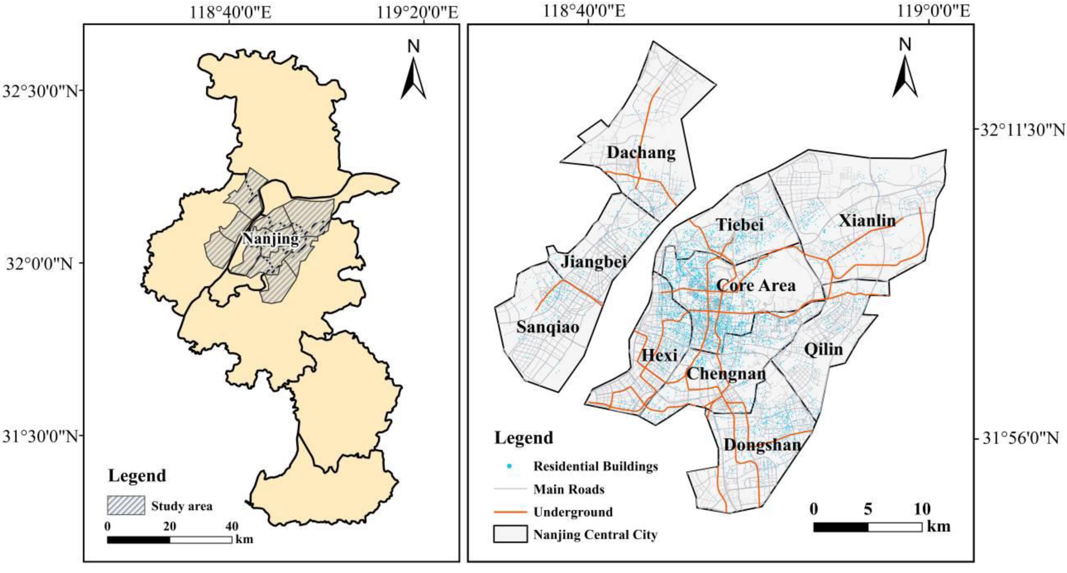
2.1. Study Area

Nanjing is a national historical and cultural city and the central city of the Yangtze River Delta. It has 11 municipal districts and 1 national new district (Jiangbei New District) under its administration. The catering industry occupies an important position in Nanjing’s service industry. According to the relevant data released by the Nanjing Bureau of Statistics, the turnover of the accommodation and catering industry in 2019 was RMB 91.2 billion, an increase of up to 14.1% year-on-year, accounting for 14.86% of the total retail sales of consumer goods (http://tjj.nanjing.gov.cn/) (accessed on 21 August 2022). The urban construction in Nanjing shows a typical expansion to the outer circle [26,37,38]. Since the 1990s, Nanjing’s urban planning tasks have focused on transforming lagging infrastructure, emphasizing the construction of new areas alongside the transformation of old cities. Nanjing has planned to form a spatial development pattern of “one main city, one new city and three sub-cities” in the city. It is necessary to study the relationship between residential and catering in Nanjing as a case study, which can provide practical guidance for cities facing functional decommissioning and rapid transformation to deal with spatial conflicts between commercial and residential spaces in a coordinated manner.

The central urban area of Nanjing, as defined in the Draft Nanjing Urban Master Plan (2018–2035), was used as the study area. The area includes ten functional zones (Core, Tiebei, Xianlin, Qilin, Chengnan, Dongshan, Hexi, Sanqiao, Jiangbei and Dafang) to accommodate the latest planning policies (Figure 1). These areas account for 12% of the city’s area, while the total population reaches 80% of the city’s resident population. Moreover, these areas are also where the most active consumer behavior occurs and where urban renewal and restaurant expansion are mainly concentrated.

2.2. Data Sources

(1)

Big data (web data) provide more accurate real-time merchant and location information than small data (statistical data, questionnaire and interview data, and industry yellow pages). VW Dianping (www.dianping.com) (accessed on 28 August 2022) is the leading lifestyle information and trading platform in China and was the first independent third-party consumer review website established in the world. We first obtained the restaurant industry data from VW Dianping (https://www.dianping.com/) through a Python program and accessed on 30 August 2022. The data fields include attributes such as the restaurant name, type, average per-person consumption price, opening time, and latitude and longitude. In addition, there are significant differences in the factors that need to be considered for the location of different grades of restaurants [39]. We divided the restaurant industry into different grades in order to compare and explore the similarities and differences in their exhibited adsorption patterns and applied the Jenks natural breakpoint method to classify the restaurant industry into 3 grades: high-grade restaurants (HRs) (84–635 RMB/person), mid-grade restaurants (MRs) (37–84 RMB/person) and low-grade restaurants (LRs) (8–36 RMB/person).

(2)

Housing information was collected by data crawling from the Anjuke website (https://nanjing.anjuke.com/) and was accessed on 14 September 2022. They mainly include attributes such as the name of the residential building, the unit price of the transaction and the year in which the house was built. We obtained the latitude and longitude by using the geocoding function provided by Gaode Map.

(3)

POI data have the characteristics of a small volume and accurate location information and are widely used in the identification of urban functional areas and the analysis of interactions between elements within the city [40]. The POI data in this study were obtained through the Gaode Map API (https://lbs.amap.com/) and were accessed on 23 September 2022. We obtained backup data for historical years through an application, and there are 7 categories: public facilities, shopping services, financial and insurance services, living services, sports and leisure services, accommodation services, and transportation facilities services (

Table 1. Number and classification of POIs.

POI Categories	POI Subclasses	Number in 2012	Proportion in 2012	Number in 2020	Proportion in 2020
Catering Services	Chinese restaurants, fast-food restaurants, cafes, teahouses, foreign fast food, foreign restaurants, snacks, tea and juice	9498	21.48%	19,304	26.16%
Public Facilities	Schools, hospitals, libraries, public toilets, public telephones, newsagents	1675	3.79%	2296	3.11%
Shopping Services	Convenience stores, specialty shops, electronic shops, cultural shops, home building markets, supermarkets, sporting goods shops, clothing shops	11,925	26.97%	18,370	24.90%
Financial and Insurance Services	Banks, insurance companies, ATMs, securities companies	3046	6.89%	5254	7.12%
Lifestyle Services	Laundries, travel agencies, logistics, post offices, repair shops, laundries, bath and massage establishments, beauty salons, post offices	10,848	24.53%	15,525	21.04%
Sports and Leisure Services	Fitness center, KTV, chess and card room, amusement park, cinema, theater	3386	7.66%	7133	9.67%
Accommodation Services	Hotels, guest houses, B&Bs	3824	8.65%	5906	8.00%

).

(4)

The geographic base information vector data were obtained from Open Street Map (OSM) (https://www.openstreetmap.org/) and were accessed on 17 August 2022. The data include administrative boundaries and road networks.

2.3. The Colocation Quotients

The global colocation quotient (GCLQ) is a measure based on nearest neighbors rather than the actual distance and was proposed by Leslie et al. [41]. It is able to avoid the influence of the overall distribution of point elements. It avoids the effect of the overall distribution of point elements and also measures the extent to which a subset of categories is spatially dependent on a subset of another category. In 2014, Cromley et al. proposed the local indicator of the colocation quotient (LCLQ), which is able to analyze the local heterogeneity of spatial processes using adaptive bandwidth [42]. It is also guaranteed that each marker point has exactly the same number of points for LCLQ estimation and can be visually represented. GCLQ and LCLQ are widely used in the study of urban crime, occupational space and industrial chains [35,43]. We used the colocation quotients to measure the ARTR. $CL{Q}_{A\to B}$ indicates the extent to which class $A$ points are attracted to class $B$ points. If the value is greater than 1, it indicates that class $A$ points are easily attracted to class $B$ points. On the contrary, if the value is less than 1, it indicates that class $A$ points tend to be dispersed from class $B$ points (

Table 2. Significant types and corresponding intervals of colocation quotients.

Type of CLQ	Description of CLQ Value Interval
Colocation—Significant	CLQ > 1 and p < 0.05
Colocation—Not Significant	CLQ > 1 and p > 0.05
Isolated—Significant	CLQ < 1 and p < 0.05
Isolated—Not Significant	CLQ < 1 and p > 0.05
Undefined	The element does not have any other elements in its neighborhood or bandwidth equal to 0

Note: p in the table represents the probability value of the random distribution of restaurant points.

). The formulas for the GCLQ and LCLQ are as follows:

$$GCL{Q}_{A\to B}=\frac{N_{A\to B}/N_A}{N_B/(N-1)}$$

(1)

$$LCL{Q}_{A_i\to B}=\frac{N_{A_i\to B}}{N_B/(N-1)}$$

(2)

$$N_{A_i\to B}={\displaystyle \sum _{j=1}^N\left\{w_{ij}{f}_{ij}/{\displaystyle \sum _{j=1(j\ne i)}^N{w}_{ij}}\right\}}(j\ne i)$$

(3)

$$w_{ij}=\exp \left(-0.5\times \frac{d_{ij}^2}{d_{ib}^2}\right)$$

(4)

where $CL{Q}_{A\to B}$ represents the extent to which restaurants are attracted to residential spaces; $N$ represents the number of all points; $N_A$ and $N_B$ represent the number of class $A$ and $B$ points, respectively; $N_{A\to B}$ represents the number of class $B$ points with class $A$ points as their nearest neighbors ($A_i$ represents the $i\text{-}\mathrm{th}$ class $B$ points); and $f_{ij}$ is a binary variable representing whether $j$ is marked as a class point (1 for yes, and 0 otherwise). Formula (4) is a mathematical expression that uses a Gaussian kernel density function to determine the spatial weights, where $w_{ij}$ is the weight of point $j$; $d_{ij}$ is the distance between the $i\text{-}\mathrm{th}$ class $A$ point and point $j$; and $d_{ib}$ is the bandwidth distance near the $i\text{-}\mathrm{th}$ class $A$ point.

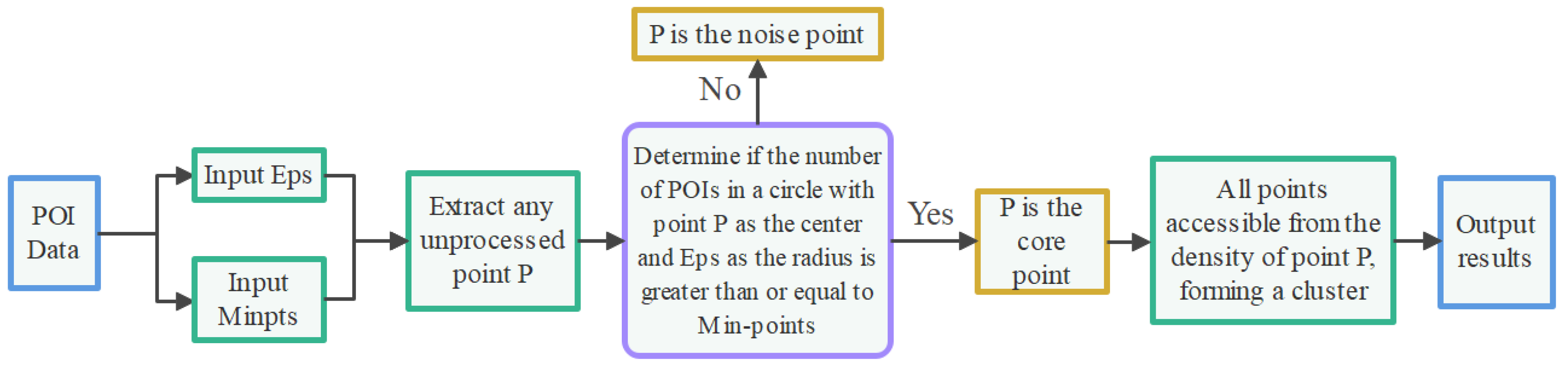
2.4. DBSCAN Clustering Algorithm

DBSCAN is a density-based spatial clustering method. It is capable of detecting arbitrarily shaped clusters in spatial datasets with noisy points. In addition, it runs faster in large-volume dataset aggregation. Therefore, it is widely used in the study of urban industrial cluster morphological characteristics’ identification and evolution [44,45]. Two important parameters of the control space cluster class are $E_{ps}$ (the range of the neighborhood of the study object within a given range) and $Mi{n}_{pts}$ (the threshold value of the number of smallest objects within the radius of the neighborhood). We identified low- and high-adsorption clusters in the restaurant industry with the help of the DBSCAN clustering algorithm. In addition, we explored the differences in the spatial and temporal evolution of different grades of restaurant clusters. The algorithm flow of DBSCAN is as follows (Figure 2).

2.5. Spatial Cold-Spot and Hot-Spot Analysis

Hot-spot analysis is a local spatial autocorrelation analysis method. It is widely used in the analysis of socio-economic as well as ecological evolution [46]. We explored the spatial clustering of high or low values of colocation quotients in the restaurant industry and their clustering patterns with the help of $G_i{}^{*}$. Our aim is to summarize the evolutionary pattern of the ARTR spatial structure even further. The calculation formula is as follows.

$$Z(G_i{}^{*})=\frac{{\displaystyle \sum _{j=1}^n{w}_{ij}{x}_j}-\overline{x}{\displaystyle \sum _{j=1}^n{w}_{ij}}}{S\sqrt{\frac{\left[\mathrm{n}{\displaystyle \sum _{j=1}^n{w}_{ij}{}^2}-{\left({\displaystyle \sum _{j=1}^n{w}_{ij}}\right)}^2\right]}{n-1}}}$$

(5)

where $x_j$ is the attribute value of feature $j$; $w_{ij}$ is the weight matrix between elements $i$ and $j$; $S$ is the standard deviation of all point element attribute values; and $n$ is the total number of elements. It is high-value spatial agglomeration if the element has a high z-score and a low p-value and low-value spatial agglomeration if the element has a negative z-score and a low p-value: the higher or lower the score, the greater the degree of clustering. If the Z-score is close to zero, there is no significant spatial clustering.

2.6. Multiscale Geographically Weighted Regression

The MGWR model adds spatially smoother variables compared to the GWR model. It sets some of the parameters as constants and the corresponding variables as global variables. It is able to consider multiple bandwidths simultaneously, which in turn enables the analysis of the scale effects of different spatial variables [47,48]. We used the MGWR model to explore the factors and scale effects that influence the spatial distribution and evolution of the ARTR. The bandwidth unit is defined as the number of grids indicating the extent of the influence of different built-environment factors. The calculation formula is as follows.

$$y_i={\displaystyle \sum _{j=1}^k{\beta }_{bwj}(u_i,v_j)x_{ij}+{\epsilon }_i}$$

(6)

where the observation unit $i$ belongs to $\left\{1,2,\cdots ,n\right\}$; $y_i$ represents the dependent variable; $x_{ij}$ represents the observed value of the $j$-th independent variable at the $i$-th unit; ${\beta }_{bwj}$ is the regression coefficient of local variables; and $(u_i,v_i)$ is the spatial coordinate of the $i$-th sample point. Several kernel functions and bandwidth selection criteria in MGWR are the same classical kernel functions and bandwidth selection criteria as in the classical GWR. We used the quadratic kernel function and the Akaike Information Criterion (AICc) method to determine the optimal bandwidth.

3. Spatial and Temporal Evolution Characteristics of ARTR

3.1. Global Characteristics of the Evolution of ARTR

We used the GCLQ as a global attractiveness measure on restaurant and residential point data for three years: 2005, 2012 and 2020. After several experiments, the bandwidths of the twenty-fifth-order neighbor and the fiftieth-order nearest neighbor were selected. In addition, we applied Monte Carlo simulations (100 times) to test for significance (

Table 3. GCLQ of restaurants attracted to residential areas.

	LR		MR		HR
Bandwidth	50	25	50	25	50	25
2005	0.8403	0.7879	0.9741	0.9098	0.9326	0.8668
2012	0.7574	0.8180	0.8818	0.8325	0.8273	0.7784
2020	0.6741	0.7383	0.8166	0.7343	0.7397	0.6727

Note: All the colocation quotients were significant at the confidence level of 0.05.

). In order to conduct cross-sectional comparison hypothesis testing to reflect the rigor and rationality of the study, we also measured the GCLQ of residential sites attracted to the restaurant industry, as shown in

Table 4. GCLQ of residential areas attracted to restaurants.

	LR		MR		HR
Bandwidth	50	25	50	25	50	25
2005	0.7239	0.7062	0.8668	0.7842	0.7822	0.7416
2012	0.6815	0.6447	0.7834	0.7241	0.7394	0.7154
2020	0.6522	0.6194	0.6971	0.6646	0.6734	0.6488

Note: All the colocation quotients were significant at the confidence level of 0.05.

. The attraction of restaurants to residential areas was greater than the attraction of residential areas to restaurants in all bandwidths, indicating that restaurants have the characteristic of being significantly dependent on the distribution of residences. The degree of absorption to residential points varied among different grades of restaurants due to the differences in consumer groups that they cater to and infrastructure costs. Mid-grade catering was the highest, followed by high-grade catering, while low-grade catering was the lowest. This may be due to the segregation of service industries with relatively low investment costs from other land parcels in order to obtain a market with easier agglomeration. This may also be related to the O2O model, since being embedded in a residential area means higher rent. In the time dimension, the degree of attractiveness of residential sites to the three grades of restaurants has been decreasing, but the rate of the decrease has been slowing down. The choice of location for catering is increasingly free from the constraints of geographical distance from neighboring consumer markets. This situation is most evident in high-grade restaurants. This is due to the fact that, on the consumer side, the concept of dining (especially luxury dining) is gradually shifting from a choice based on proximity to a focus on the dining experience, such as the service, the environment and the dishes themselves. In addition, the requirements for neighborhood spatial planning and site restrictions in new residential areas have become more stringent. This makes the layout of the catering industry more subject to the macro control of the functional area to which it belongs.

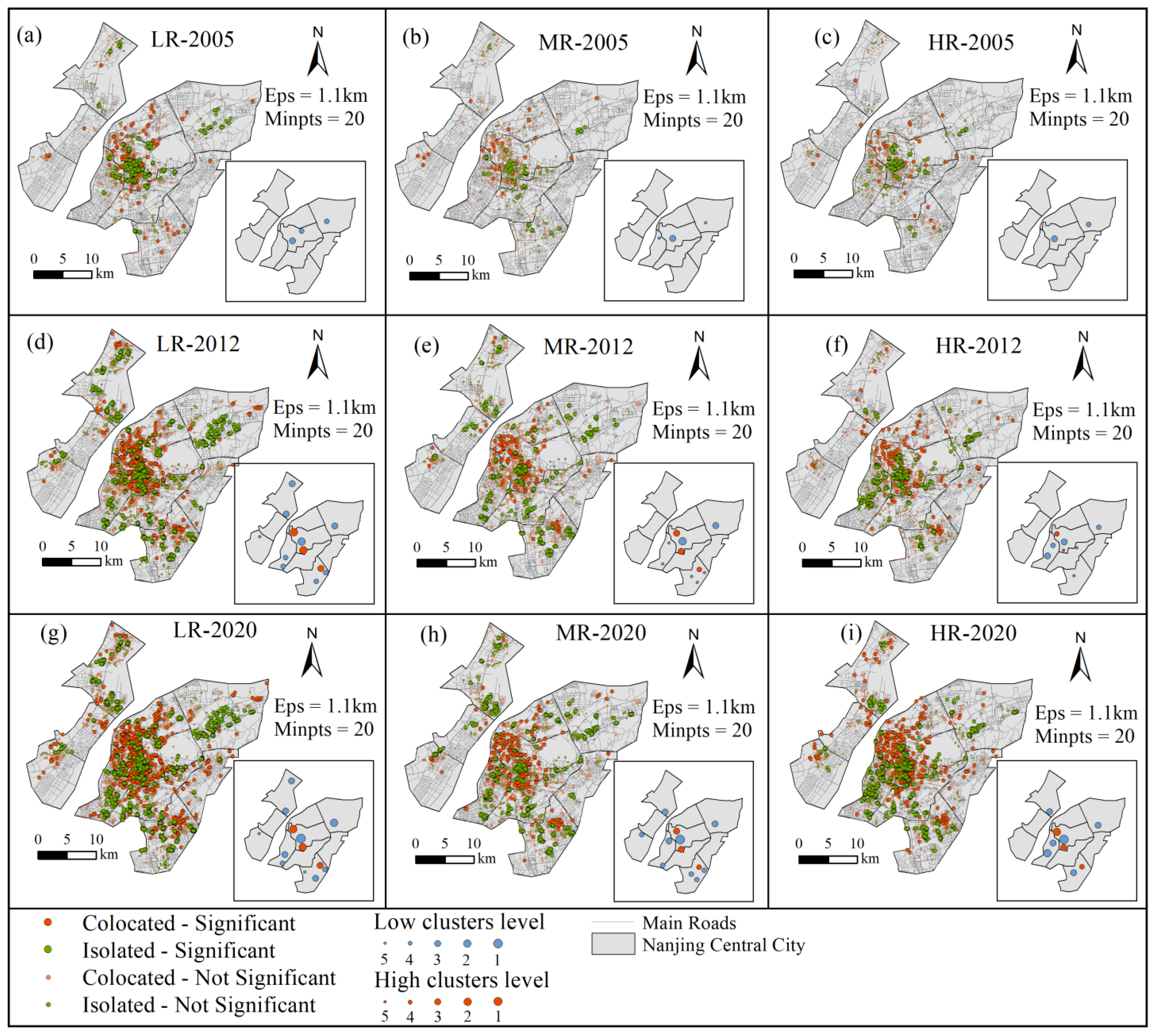
3.2. Local Characteristics of the Evolution of ARTR

We measured the extent to which restaurants were attracted to residential housing using local colocation quotients. However, it is not possible to visualize the spatial regularity characteristics. We therefore continued to use the DBSCAN clustering algorithm to identify clusters for different grades of restaurants. We classified clusters with fewer than 30 restaurants as five-level cluster centers, 31 to 50 restaurants as fourth-level cluster centers, 51 to 80 restaurants as third-level cluster centers, 81 to 150 restaurants as second-level cluster centers and more than 150 restaurants as first-level cluster centers based on the natural breakpoint hierarchy and the actual clustering results.

According to the statistics of the LCLQ (

Table 5. Parameters related to LCLQ of ARTR.

Time	Grade	Isolated Count	Colocated Count	Min	Median	Max	Mean	Std	Total
2005	Low	868	68	0	0.73	1.38	0.74	0.27	1972
	Middle	216	29	0.09	0.78	1.26	0.88	0.24	814
	High	309	31	0.13	0.72	1.25	0.74	0.22	756
2012	Low	2657	368	0	0.60	2.42	0.64	0.50	4520
	Middle	924	119	0.02	0.70	1.59	0.75	0.33	2745
	High	948	117	0	0.65	1.50	0.70	0.35	2233
2020	Low	5573	787	0	0.46	3.19	0.59	0.66	9687
	Middle	1998	228	0	0.55	1.87	0.63	0.41	4621
	High	2490	325	0	0.50	1.94	0.62	0.45	4996

Note: Both isolated count and colocated count are significant at 95%.

), the mean and median values of each grade of the restaurant industry were around 0.7, and the number of isolations was much greater than the number of colocations. Therefore, the extent of attraction remained generally low. The LCLQ values started to decline overall as time progressed, but the rate of decline gradually slowed down. The standard deviation values for the LRs were the largest and had the highest rate of change over the years, indicating that they were more sensitive to changes in the built environment. Moreover, the heterogeneity of their spatial distribution was more pronounced. In contrast, the performance of MRs and HRs was not as obvious. Figure 3 reveals the spatial and temporal evolution of the ARTR measured by the LCLQ method. The DBSCAN algorithm was used to identify the spatial structures of low- and high-adsorption catering clusters. The cross-sectional results of this indicate the spatial layout characteristics of the ARTR for different grades of restaurants. The longitudinal results represent the evolution of the ARTR pattern in the time dimension. The main parameters of DBSCAN were identified by the K-dist diagram and are marked in the diagram. The main parameters of DBSCAN identified by the K-dist plot $E_{ps}$ and $Mi{n}_{pts}$ are indicated in Figure 3. To further summarize the evolution of the ARTR spatial structure, we used the G-index to explore the local spatial autocorrelation of the ARTR for different grades of restaurants. Its spatial visualization results are shown in Figure 4.

In general, the center–periphery structure of the restaurant industry in Nanjing is obvious. The concentration density of the restaurant industry is distributed in a gradient from the city center to the periphery. In addition, a multi-core layout has gradually formed over time.

In 2005, restaurants with low ARTR values formed large clusters in the urban core. This was probably due to the high degree of specialization in the Xinjiekou CBD of Nanjing. The restaurants closely surrounding the low-absorption cluster were embedded in the residential area of the Xiaguan area, which resulted in significantly high values of the LCLQ (p < 0.05). However, no high-absorption clusters were formed. The LCLQ of LRs varied depending on the timing of the completion of the urban sub-center. For example, high-value hot spots were identified in the Jiangning Dongshan sub-city (the mean value was 1.08), which was lagging behind in planning concepts. In contrast, a cold spot of low-value clustering was identified in Qixia New Town (the mean value was 1.08), which has clear functional zoning. The mid-grade and high-grade restaurants, on the other hand, were generally segregated (the mean values were 0.68 and 0.64) and not sensitive to the built environment of the sub-center (the standard deviations were 0.24 and 0.22). In addition, according to the DBSCAN clustering results, low-adsorption clusters were identified in Xinjiekou CBD and Xianlin New Town (the mean values for LRs were 0.45 and 0.38, respectively), while high-adsorption clusters had not yet been formed. The Xinzhuang area formed a low-absorption tertiary cluster, which was mainly influenced by the large shopping centers. MRs and HRs in the Xianlin area, which would have been in isolation, were identified as hot spots in the ARTR hot-spot analysis due to the barrier effect of the Zhongshan scenic area and the fact that their own LCLQs were not significantly low.

In 2012, all three grades of high-adsorption clusters in the restaurant industry began to be identified. In terms of LRs, the number of catering businesses in Tiebei and Chengnan had increased significantly, and they were highly embedded within residential areas (the mean values were 1.23 and 1.54, respectively). With the accelerated construction of Hexi New Town, Xianlin New Town and Dachang, a low-value agglomeration center of ARTR for LRs was formed in the sub-center area (the mean values were 0.65, 0.36 and 0.48, respectively). There were differences in the level and concentration scale of the restaurant industry in different sub-centers, which were mainly related to the time of the development and construction of each sub-center. The agglomeration of Jiangbei New Town was dominated by LRs, while the development and construction of Hexi CBD made HRs start to gather in the Hexi area, forming a medium-sized low-absorption cluster (the mean value was 0.73). According to the hot-spot analysis chart, a low–high–low circular structural feature of low-end catering cluster adsorption was formed, while the structural feature of mid-grade and high-grade catering was not obvious. The hot-spot analysis mainly identified the hot spots of ARTR for MRs in the Xiaguan area and cold spots in the core area. However, HRs were more complete, with a single core cold spot. They were surrounded by hot spots that represent high-value clusters.

The spatial distribution of the ARTR in 2020 had more significant structural characteristics compared to 2012. The specific features were as follows: (1) The concentration of the restaurant industry in the core area had enhanced, while the scope of the high-adsorption clusters in the old city immediately adjacent to the core area of Xinjiekou continued to expand outward. Specifically, it extended to the northeast and south of the city and connected with the sub-center of the city to form one piece. (2) The first-level cluster centers and the second-level cluster centers basically formed a whole, which benefited from the improvement of the rapid transportation system and infrastructure construction, presenting a continuous spatial envelope structure. However, the ARTR for different grades of catering presented different characteristics, among which the LRs formed an obvious spatial structure, and MRs presented two cores of high values and low values, while the high-adsorption circle of HRs was more inclined to a semi-encircling structure. (3) The attractiveness of residential spaces to different grades of restaurants showed a diverse distribution in the fringe areas due to the different target consumer groups and the time of completion. For example, there were sporadic clusters of high adsorption in the Dongshan District of Jiangning (the LCLQ’s standard deviation changed from 0.74 to 0.89). The relationship between residential space and the service industry in the Dongshan area should be reasonably improved through planning and construction in the future, thus promoting the sustainable development of the community. The relevant functional agencies in Qixia New Town, Jiangbei Core Area and Hexi Area should reasonably consider how to optimize the accessibility of living space and the service industry under the concept of a living circle.

3.3. Analysis of Factors Influencing the Spatio-Temporal Heterogeneity of ARTR

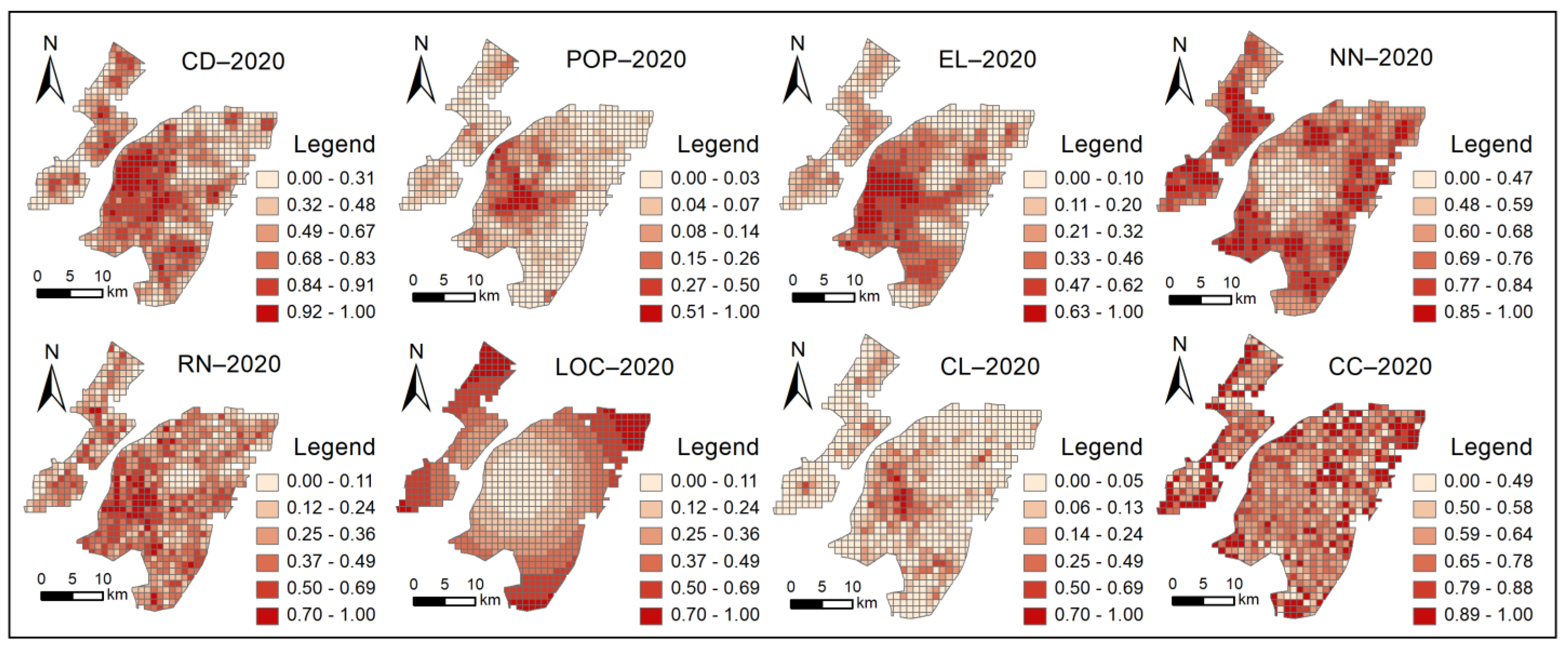
3.3.1. Indicator Selection

Eight dimensions of influencing factors were selected for the geographically weighted regression analysis based on the literature review (

Table 6. Selection and description of explanatory variables.

Factor Dimensions	Indicator Variables	Variable Interpretation	2012 VIF	2020 VIF
Commercial diversity (CD)	Diversity index of commercial facilities in the grid	$POI{M}_i=-{\displaystyle \sum _{j=1}^n{P}_{i,j}}\times \ln P_{i,j}$	1.632	1.524
Population level (POP)	Population density	Ratio of the number of people in the grid to the area	1.876	1.619
Economic level (EL)	House price level	Average room rates within the grid	2.577	3.622
Neighborhood newness (NN)	House completion time	Average completion time of houses in the grid	3.418	2.165
Road network level (RN)	Road network density	The ratio of the total length of the road in the grid to the area of the grid	3.214	3.049
Location condition (LOC)	Distance from the city center	Distance from square grid center to city center (Xinjiekou)	4.195	4.455
Clustering level (CL)	Nearest neighbor index of catering industry	$NN{I}_i=\overline{D_{oi}}/\overline{D_{ei}},\overline{D_{ei}}=0.5/\sqrt{n_i/A_i}$	2.686	3.274
Commercial competition (CC)	Other commercial POIs’ density	Ratio of the number of other commercial POIs to the number of restaurants in the grid	2.418	2.246

$P_{i,j}$ denotes the weighted percentage of the $j$th POI in grid $i$; $POI{M}_i$ is the SHDI of the $i$th grid; $NN{I}_i$ is the nearest neighbor index of the $i$th grid; $\overline{D_{oi}}$ is the average of the nearest neighbor distance of the restaurant elements in the $i$th grid; $\overline{D_{ei}}$ is the expected nearest neighbor distance of the restaurant elements in the $i$th grid; $n_i$ and $A_i$ are the number of samples in the grid and the area of the grid, respectively.

).

(1)

Commercial Diversity: The land-use mix is a useful indicator to measure the level of functional zoning in a city and, to a certain extent, reflects the level of neighborhood vitality and commercialization [49]. We used the commercial land-use mix as an indicator to explore whether commercial diversity can increase or decrease the ARTR.

(2)

Population Level: The population density represents the consumption demand of a geographical unit. As a consumer-oriented service, catering tends to be laid out in areas with higher population densities to approach higher clientele. However, a high population density will bring intense competition for spatial location [21]. The population density was selected as a variable to explore the spatial heterogeneity of its impact on the ARTR.

(3)

Economic Level: The residential price can roughly reflect the consumption ability of the residential population and the basic rent level of the neighboring areas, which in turn can characterize the economic level of the grid [50]. Based on the neighborhood house prices obtained from the web platform, the house prices within the grid were calculated by inverse distance weighted interpolation (IDW) so that we could investigate whether there were spatial and temporal differences in the influence of the residential class level on the ARTR.

(4)

Neighborhood Newness: The time of residential completion reflects the timing of the planning and development of the area, and the difference in planning concepts and strategies between different periods will directly affect the spatial relationship between restaurants and residential spots. Usually, the later the planning period, the more emphasis that is placed on the zoning of functions, while planning in an earlier period takes the needs of the citizens themselves as the leading guide.

(5)

Road Network Level: The layout of the catering industry is highly correlated with the intra-city transportation system [51,52], and the increase in regional accessibility may weaken the influence of housing on the location choice of the catering industry through the “spatial and temporal compression” effect. The road network density is an important indicator to reflect the level of regional traffic access, and traffic variables are measured by calculating the road network density.

(6)

Location Condition: The central city of Nanjing conforms to the urban territorial differentiation rule of the multi-core model. Several new cities are distributed around the city center, serving local economic and social functions. This indicator explores the territorial differentiation pattern of ARTR under the multi-core model. Xinjiekou is a widely recognized landmark of the Nanjing city center, and the distance of the grid center from Xinjiekou was assigned to the grid for measurement.

(7)

Clustering Level: Restaurant clusters are geospatial clustering phenomena formed by the catering industry, and they attract and link to each other in order to reduce operating costs and obtain the maximum profit [53]. The degree of agglomeration affects the location choice of the catering industry, and the degree of agglomeration was calculated by the nearest-neighbor index within each grid.

(8)

Commercial Competition: The location of the catering industry is also attracted by other elements, such as commercial centers, transportation locations, etc., which will cause it to shift away from residential centers to locations that can increse profits [53]. The density of other commercial service facilities in the grid was selected as the independent variable of spatial competition.

All indicators in this paper have been standardized, and the regression coefficients of different indicators can be compared with each other. Before the variables were introduced into the model, the eight explanatory variables were tested for cointegration. It was found that the VIF of each explanatory variable was less than 10, and there were no apparent multiple-cointegration problems. The standardized independent variable dataset for 2020 is visualized in Figure 5.

3.3.2. Model Selection and Comparison

We first analyzed the influencing factors of attractiveness using OLS models and constructed GWR and MGWR models using the same variables to identify the influencing factors. The following table shows the parameter estimates of the residual sum of squares, AICc and adjusted R² for each model (

Table 7. Comparison of OLS, GWR and MGWR model metrics.

		OLS			GWR			MGWR
Year	Level	RSS	AICc	Adjusted R2	RSS	AICc	Adjusted R2	RSS	AICc	Adjusted R2
2012	Low	342.18	−3165.84	0.436	283.45	−3341.12	0.743	236.49	−3429.65	0.871
	Middle	405.61	−4284.46	0.378	362.12	−4519.54	0.684	324.84	−4710.89	0.792
	High	377.48	−3412.48	0.455	317.45	−3874.46	0.719	288.69	−3962.81	0.896
2020	Low	508.49	−5221.18	0.365	463.55	−5648.61	0.692	416.59	−5841.64	0.794
	Middle	477.38	−4815.64	0.348	414.37	−5229.81	0.745	396.44	−5397.18	0.882
	High	516.37	−5617.39	0.337	486.49	−6018.52	0.731	465.28	−6294.44	0.843

). The multiscale geo-weighted regression model (MGWR) has higher goodness-of-fit R² and lower Akaike Information Criterion (AICc) values than the geo-weighted regression (GWR) and ordinary least-squares (OLS) models. The regression results are closer to the true values in terms of the residual sum of squares, showing its advantages over the other two models. Therefore, the MGWR model was chosen to explore the spatial heterogeneity of ARTR influences in this study.

3.3.3. Commercial Diversity and Population Level

We finally selected a 1 km ∗ 1 km grid as the study unit through repeated operations and assigned LCLQs to the grid by using the inverse distance weighted interpolation (IDW) method. We used MGWR2.2 software to calculate the above eight categories of influencing factors and used ArcGIS10.7 software to spatially visualize and express the variables. The Jenks natural breakpoint method was used to classify the coefficient values into six levels. Due to the difficulty of obtaining POI and road network data for 2005 and the limitation of the length of the article, this part of the analysis selected two categories, LR and HR, in 2012 and 2020 for the study. The results are shown in Figure 6. The mixed land use essentially acts positively on the ARTR, and the regression coefficient interval distribution is from −0.46 to 0.58, which shows that the overall magnitude of the effect is not significant. However, there are subtle differences with time. The spatial distribution of the regression coefficients decreases from west to east, which indicates that the increase in the land-use mixture along the river can effectively promote the enhancement of the ARTR, whether it is an HR or LR. The ARTR and land-mix regression coefficients for HRs gradually extend to inner Jiangnan. Specifically, the regression coefficient of LRs decreased over time and contracted to between 0.12 and 0.26; the effect of commercial diversity on HRs is generally smaller than that on LRs, with its regression coefficient located between 0.05 and 0.28. The area along the river shows apparent high-value clustering, and the lowest value is located near the Qixia district, probably due to the late planning of Qixia New City; the residential space and service industry show separation characteristics.

The regression coefficient intervals of the population level for LRs and HRs were −0.90~0.34 and −0.64~0.16, respectively, in 2012. Spatially, it shows core–edge characteristics, with a lower degree of influence in urban centers and a more pronounced positive effect in the fringe suburbs. Specifically, the response of the ARTR for LRs to the population density was more obvious, and the high values were mainly concentrated in Xianlin University City, Tangshan New Town and the Jiangbei Pukou area, which indicates that the increase in population density in suburban areas will prompt the establishment of restaurants near residential space. In the temporal dimension, the central low values for both LRs and HRs continued expanding to the periphery. The scope affected by the population density decreased, but the polarization of the high-value areas in the suburbs became more evident as the catering industry continued clustering.

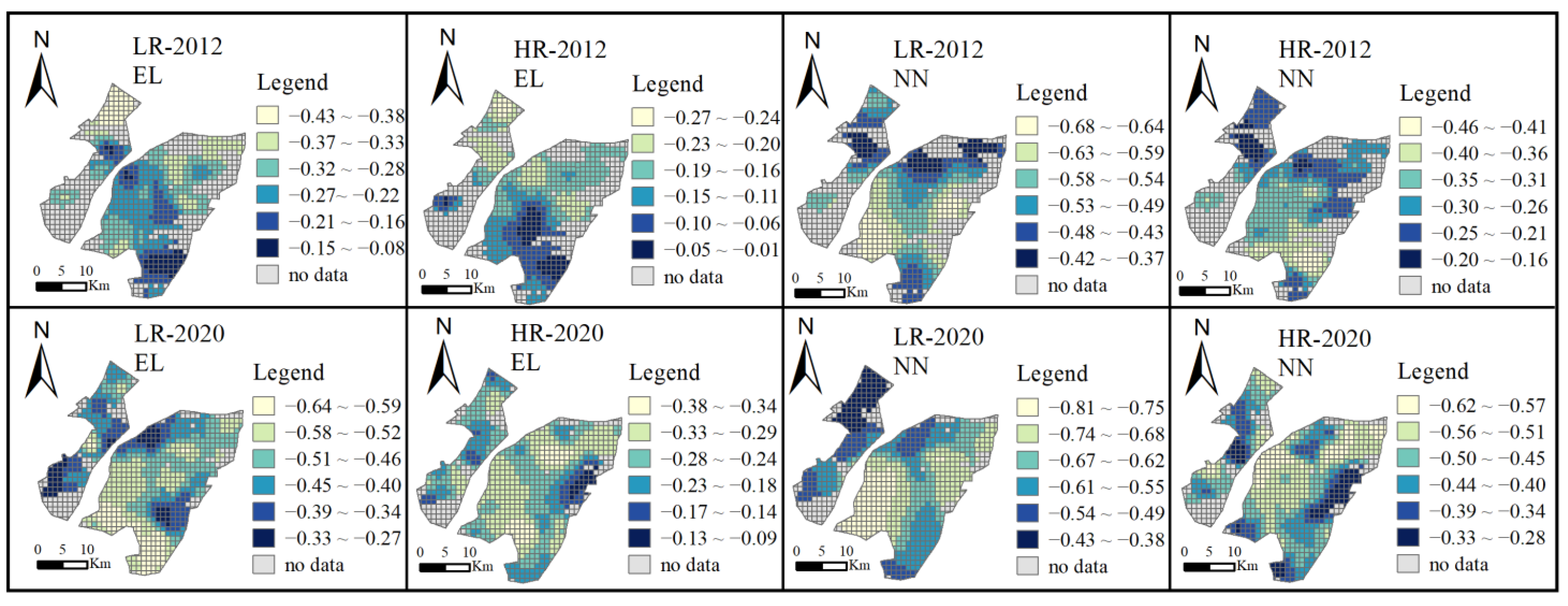
3.3.4. Economic Level and Neighborhood Newness

The regression coefficients of the economic level on the influencing factors of low-grade and high-grade catering ARTR are negative throughout the whole area (Figure 7). The regression coefficient intervals of ARTR for LRs and HRs in 2012 were −0.43~−0.44 and −0.27~−0.01, respectively. In terms of spatial distribution, the high-value areas were concentrated in old urban areas such as Qinhuai and Jiangning Dongshan. Compared with HRs, the housing price values were higher in Jiangbei New Area and Xiaguan area for ARTR with LRs, while the low values were concentrated on some urban edges with relatively low planning and management levels. The regression coefficients changed more dramatically in value and space over time, probably due to the dramatic change in the house price factor between 2012 and 2020. The regression coefficients of −0.64 to −0.27 and −0.38 to −0.09 for the low- and high-level restaurant ARTR, respectively, suggest an increasingly negative effect of consumption power on sorption. In the spatial distribution of the 2020 regression coefficients, the regression coefficient values of the Hexi area became low due to the change in the function of the plot from industry to business and the surge in house prices influenced by the market and the surrounding infrastructure, which shows a negative effect on the adsorption power. However, the urban expansion of Pukou New District gradually improved, which shows a positive effect on the adsorption power.

The degree of neighborhood newness represents the temporal difference in the planning and management philosophy of the area. According to Figure 4, the regression coefficients of the neighborhood newness on the adsorption factors are negative throughout the whole area. The negative effect becomes more and more evident over time, which is similar to the development history of planning in Nanjing, indicating that the older the neighborhoods are, the better the embeddedness of the catering industry. The zoning plan implemented in recent years has achieved good results. Specifically, the regression coefficients of ARTR for low-grade restaurants (−0.68 to −0.37) and HRs (−0.46 to −0.16) are more similar in 2012, while the negative effect of the neighborhood build-up time on LRs is more pronounced. In general, the spatial distributions of the two types of regression coefficients are relatively similar: they are higher on the northern and southern sides of the city and lower in the downtown core. Specifically, the influence of neighborhood newness in the Yanziji area, Qixia New Town and the south of Jiangning is insignificant. However, its negative effect is pronounced in the core area. The regression coefficient values and spatial patterns changed significantly in 2020, and the negative effect of neighborhood newness on the ARTR is enhanced in the Dachang district due to its early completion and relatively poor planning, coupled with the large number of HRs moving in between 2012 and 2020.

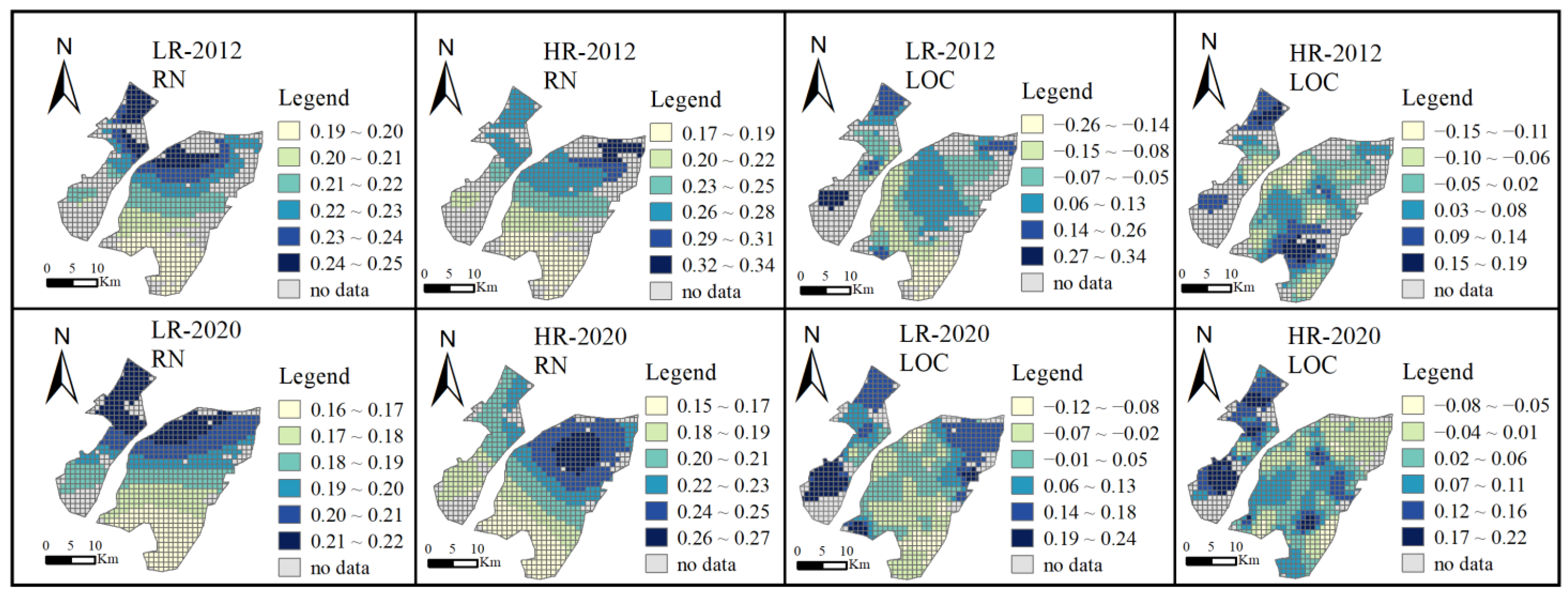
3.3.5. Road Network Level and Location Condition

The overall impact of the road network level on the ARTR in 2012 was positive, roughly between 0.19 and 0.34, showing a spatial distribution trend of high values in the south and low values in the north, but the spatial heterogeneity was not obvious (Figure 8). In the earlier-developed Yanziji area and Dafang area, which are high-value areas, the density of the road network had a greater impact on the ARTR for LRs, implying the more favorable integration of restaurants with residential space. The regression coefficients of the ARTR for HRs were in the northeastern part of the central city. We speculate that in areas with low road network density levels, higher road network levels can contribute to the rise in ARTR for HRs. Regarding the time dimension, the spatial distribution coefficients of the regression coefficients do not change much and are still mainly characterized by high values in the north and low values in the south. Comparing the regression coefficients of the ARTR with HRs and LRs, the road network density has a greater effect on the adsorption of high-level restaurants.

The regression coefficients of location conditions were more widely distributed (Figure 7). In 2012, the regression coefficients of ARTR were −0.26~0.34 and −0.15~0.19, respectively. The spatial heterogeneity of the overall magnitude of the effect was more obvious, mainly showing a pattern of low values in the middle and high values around it. The spatial distribution of the regression coefficients of ARTR for HRs showed a multi-core pattern, with high values of agglomeration in the Jiangning urban area and Dafang district and low values of agglomeration in the main urban areas, such as Gulou and Qinhuai. From the spatial dimension, the regression coefficients of ARTR for LRs showed a more obvious circular structure, and a farther distance from the city center increased the adsorption of LRs in suburban areas to residential areas. In contrast, the positive effect of the location factor on the adsorption of HRs was more significant in Jiangbei. The regression coefficients of both underwent an interval range reduction over time, indicating that location factors’ influence on the ARTR gradually decreased.

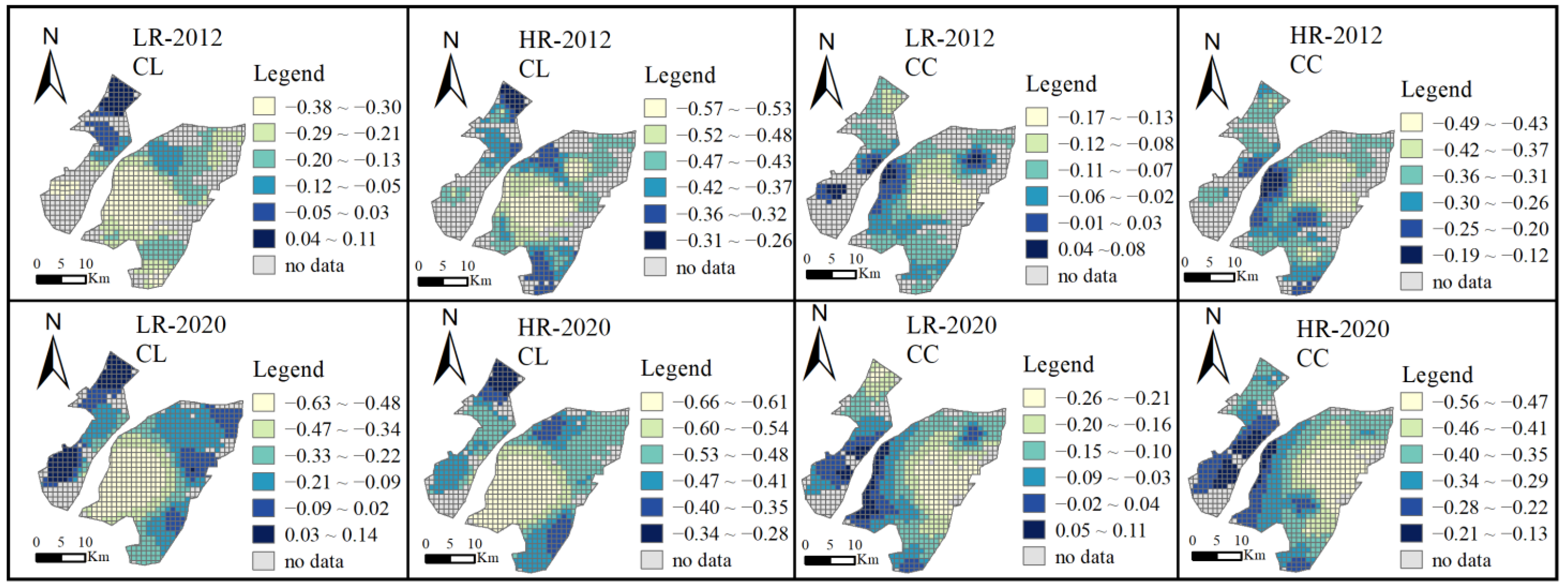
3.3.6. Clustering Level and Commercial Competition

The impact of the spatial agglomeration of the catering industry on the ARTR varied by location, and its regression coefficients showed a clear spatial arrangement with low values in the middle and high values in the surrounding circle (Figure 8). However, they are all negative, which indicates that the segregation effect caused by spatial agglomeration is more significant. In 2012, the regression coefficients of spatial agglomeration of ARTR were −0.38~0.11 and −0.57~−0.26 for LRs and HRs, respectively, and Jiangbei Dachang Area was the low-value agglomeration area for both types of ARTR. In addition, the high values of regression coefficients of ARTR for HRs were also concentrated in the southern Jiangning and Yanziji areas. It is possible that the negative effect of spatial agglomeration is relatively small because these areas are dominated by tourism functions and have larger green areas, while the density of the catering industry was low. The circular structure did not change as time continued to evolve, which indicates that urban renewal and expansion did not change the effect of agglomeration on the ARTR. The positive effect of agglomeration in the Xianlin and Tangshan areas on the ARTR was more pronounced in lower grades than in higher grades.

The spatial competition in the catering industry had an overall negative effect on the adsorption of the catering industry, with regression coefficients of −0.17 to −0.08 and −0.49 to −0.12 for LRs and HRs in 2012, respectively (Figure 9). In general, competition in other types of service industries will have a more significant effect on the ARTR, and the high-value areas of the regression coefficients were mainly concentrated in the area along the river. This might be because the land along the rivers was highly occupied, the degree of intensification was higher, the catering industry was more developed, and it was the dominant industrial sector among all types of commercial facilities, so it had higher adsorption to the residential area. In 2020, the regression coefficient decreased slightly, and the role of competition in the ARTR was always present and increasing in intensity. Spatially, with the vertical expansion of urban land, the area with high values of regression coefficients continued to expand to the southern riverine areas, and the regression coefficients of ARTR for both HRs and LRs showed similar patterns.

3.3.7. Scale Effects of Influencing Factors

For the factors influencing the attractiveness of residential space to the catering industry, we further conducted a scale effect analysis.

Table 8. Bandwidth of influencing factors for MGWR model estimation.

Variables	MGWR-LR 2012			MGWR-HR 2012			MGWR-LR 2020			MGWR-HR 2020
	BW	BP (%)	Scale	BW	BP (%)	Scale	BW	BP (%)	Scale	BW	BP (%)	Scale
CD	255	43.29	Local	208	35.31	Local	548	70.89	Global	605	78.27	Global
POP	136	23.09	Local	182	30.90	Local	252	32.60	Local	278	35.96	Local
EL	73	12.39	Local	86	14.60	Local	98	12.68	Local	102	13.20	Local
NN	218	37.01	Local	106	18.00	Local	316	40.88	Local	142	18.37	Local
RN	512	86.93	Global	533	90.50	Global	677	87.58	Global	686	88.75	Global
LOC	81	13.75	Local	74	12.56	Local	92	11.90	Local	86	11.13	Local
CL	132	22.41	Local	187	31.75	Local	158	20.44	Local	267	34.54	Local
CC	107	18.17	Local	184	31.24	Local	209	27.04	Local	255	32.99	Local
GWR	166	28.18	—	185	31.41	—	274	35.45	—	301	38.94	—

shows the bandwidths of the different drivers in the GWR and MGWR models, which represent the differences in the scales of action of each variable. The bandwidths of the GWR for LRs and HRs were 166 and 185 in 2012, accounting for 28.18% and 31.41% of the total sample size, respectively, while they accounted for 35.45% and 38.94% in 2020. This shows a trend toward a global shift in each influencing factor in the time dimension, but the magnitude of the shift is not significant. Specifically, for each influencing factor, the bandwidth varies significantly, and the scale of influencing factors they reveal is significantly different. Based on the bandwidth scale as a percentage of the global sample (BP) and the corresponding administrative district width, it can reflect that the drivers show scale effects at two levels: global scale (BP > 50%) and local scale (BP ≤ 50%). The level of the road network (86.93%) is the macroscopic variable at the global level in 2012, while commercial diversity, population level, economic level, neighborhood newness, location condition, clustering level and like-for-like competition are micro-local variables with significant regional differences and a highly spatially non-smooth relationship with the ARTR, which is consistent with the range and distribution of coefficients in the regression coefficient results. From the perspective of time evolution, the level of the road network always acts on the ARTR at a more macroscopic scale, and the indicative scale of commercial diversity undergoes a shift from local to global, probably because the full-scale construction and expansion of commercialized supporting complexes within the central city raised its scale of influence. The location conditions and economic level are stable at a more microscopic scale, probably due to the apparent heterogeneity in the spatial distribution of house prices and specific locations and the more drastic local changes in economic factors due to the rapid development of the economy and real estate.

4. Discussion

Unlike the study of the relationship between residential areas and employment, the spatial relationship between the service industry and residential space is a unified entity with both benefits and negative externalities [2]. On the one hand, some scholars advocate the neighborhoodization of residential space, which is a powerful way to enhance urban vitality and boost consumption by mixing the vertical use of neighborhoods with a high degree of embeddedness [54]. In contrast, functionalist-oriented scholars believe that zoning can achieve the optimal allocation of urban resources and will significantly improve the efficiency of intensive urban management [55]. For example, community neighborhood centers have been successfully practiced in Suzhou Industrial Park. Since “physical online” has become a popular trend, consumers will pay more attention to the physical experience. A new round of changes will occur in the urban ARTR, so it is necessary to dynamically adjust the planning scheme. Most of the influencing factors we calculated are localized, which requires a more refined approach to neighborhood issues. The relationship between agglomeration and dispersion, diversity and specialization should be precisely handled in the future according to the built environment and socio-economic characteristics of different neighborhoods.

The analysis of the spatial distribution of ARTR values can provide some indication of urban development. From the results of our study, the distribution of restaurants embedded in residential space in the core–periphery of CBD is a place of neighbor avoidance. Conflicts are also extremely likely to occur. This “fragile zone of coexistence” therefore places greater demands on the management of noise, pollution emissions and consumer orders in the catering sector. We found relatively low LCLQ values in the urban fringe. New town planning at the periphery ignores the accessibility of services. This may lead to a reduction in the efficiency of land resource allocation. It may even hold back the development of compact cities. These problems can be solved by increasing the density of the road network and reducing excessive agglomeration and competition. In addition, the planning of new towns should also take into account the accessibility of meals for vulnerable groups, such as the elderly and students. The question of how to balance equity and efficiency in the context of function-oriented new town planning is worth considering.

Our proposed concept of ARTR can be one of the indicators for the fine measurement of urban functional zoning at small scales. In addition, it can be applied to geography, urban sociology and urban economics, providing new ideas for solving the conflict between negative externalities of business and community residents and providing some empirical insights to local policymakers. In addition, we focused on the active role of residential sites rather than the interaction between the two elements to measure the ARTR and its evolution mechanism from a spatial evolution perspective rather than a static one. In the future, urban planners and geographers should reasonably regulate the relationship between residential areas and service industries so as to minimize the negative externalities of service industries and maximize the economic and social benefits of spatial land resource allocation.

However, our study still has the following limitations: (1) Limited to the data availability, we only discussed the spatial relationship between the service industry and residential areas. In fact, the analysis of other service industries, such as accommodation, hospitals, schools and financial services such as banks and ATMs, would also be valuable and can provide a scientific and empirical basis for exploring the spatial relationship between service industries and residential space. (2) In the context of new retailing, take-out stores have become indispensable residential food and beverage businesses, so the comparison of the spatial differentiation between traditional stores and take-out stores in the central city under the influence of the O2O model and its mechanism can be explored in the future. (3) The urban renewal and planning response is a long-term policy practice process, so we need longer time series data to reflect the attractive spatio-temporal evolution process. At the same time, socio-economic and built-environment-induced changes in spatial relationships should be considered in depth so as to ascribe more universal laws and mechanisms.

5. Conclusions

We used data from VW Dianping and multi-source urban built environments in 2005, 2012 and 2020 to quantitatively measure the ARTR for different grades of restaurants using synergistic GCLQ, LCLQ and DBSCAN cluster analysis methods. In addition, we applied multiscale geographically weighted regression models to study the influencing factors and scale effects of the ARTR of restaurants in 2012 and 2020, which is crucial for scientifically formulating the relationship between urban restaurants. It is also vital for the in-depth understanding and regulation of the spatial relationship between the catering industry and residential buildings. The main conclusions are as follows.

(1)

The attractiveness of residential space in the central city of Nanjing to different grades of restaurants presents different global and local characteristics. At 50th-order bandwidth, the results of the global measurement show that MRs are the highest (the average is 0.89), followed by HRs (the average is 0.83), while LRs are the lowest (the average is 0.76). Attractiveness decreases over time due to the influence of macro-planning policies. At 50th-order bandwidth, LRs, MRs and HRs were reduced by 0.17, 0.16 and 0.19, respectively. The spatial and temporal distribution characteristics of the ARTR were analyzed by measuring the LCLQ, which formed a spatial layout with low attraction values as the core cluster, middle circles with high-value clusters and external sub-core areas as low-value clusters. The cluster level decreases from inside to outside in order.

(2)

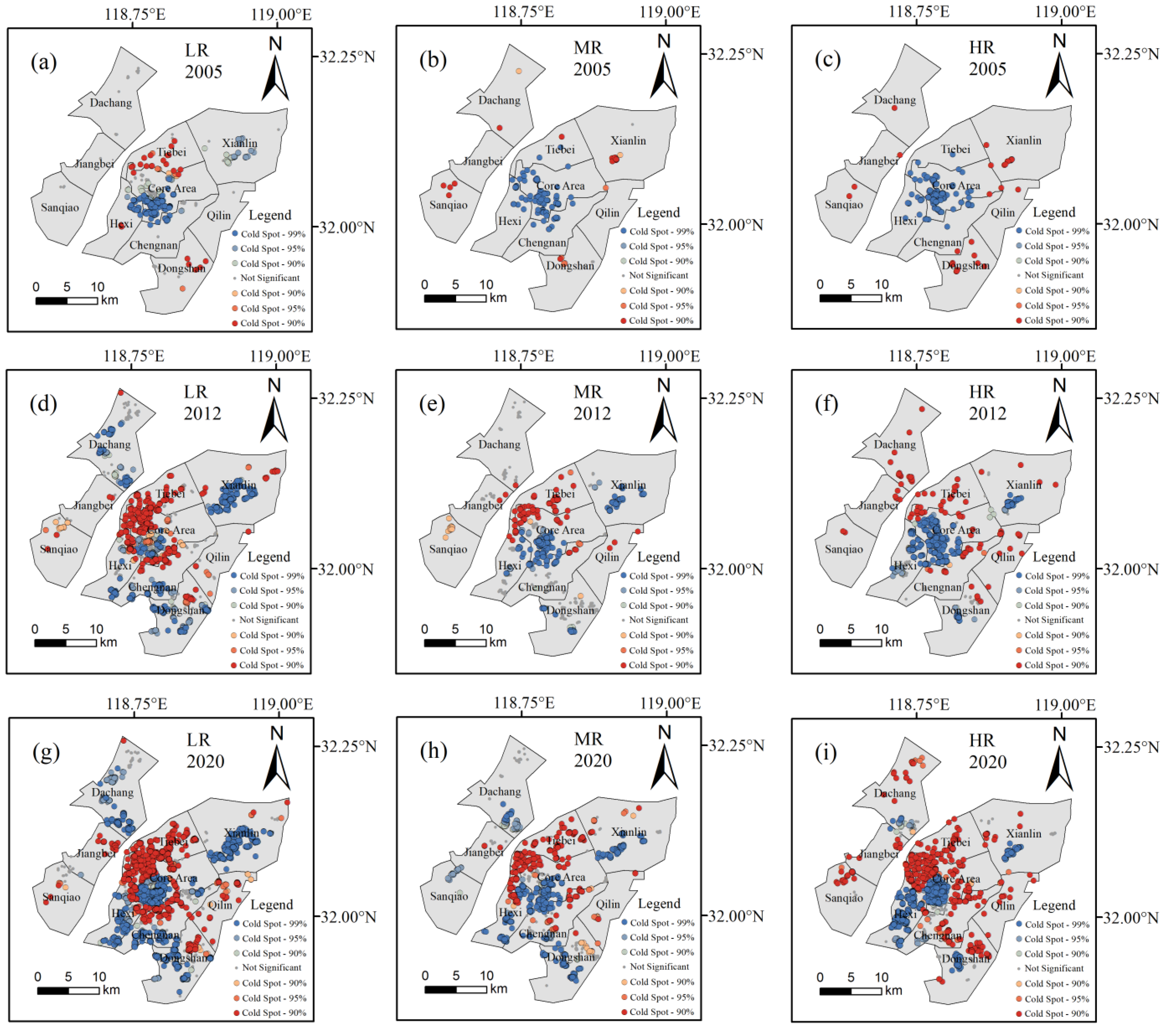
We used hot spots to analyze the spatial autocorrelation phenomenon of ARTR in the central city of Nanjing. The results show that there are also significant differences in the clustering of high and low values of the ARTR for different levels of restaurants. For example, the ARTR for LRs has a circular structure. In contrast, the ARTR of MRs and HRs shows a semi-envelope structure. The evolution trend shows that LRs are more flexible than MRs and HRs in responding to changes in the built environment in urban renewal (LCLQ standard deviation for LRs increased from 0.27 to 0.66).

(3)

The factors affecting the ARTR for LRs and HRs were analyzed from eight variables characterizing the built environment. The regression coefficients of the different built-environment factors are spatially different, with urban expansion and regeneration leading to stronger adverse effects of spatial agglomeration, competition in the service industry, the economic level and the newness of neighborhoods. The means of their regression coefficients decreased by 0.08, 0.04, 0.15 and 0.1, respectively. Unexpectedly, the road network density was more stable (the mean changed from 0.24 to 0.22). The ARTR became progressively less responsive to location conditions.

(4)

The MGWR model takes into account the diversity of the scales of action of the drivers. It effectively reduces the noise and bias of the regression coefficients. The scale effects of the drivers and the spatial heterogeneity of the degree of influence can be estimated by the variable optimal bandwidth. We further analyzed the scale effects of the drivers and found that the road network density was a constant global factor (the average scale was 88.44%). Business diversity changed from a local factor to a global factor (the scale changed from 39.3% to 74.58%), while the average scales of economic and location factors were 13.22% and 12.34%, which had strong spatial non-stationarity.

References

1. Wu, M.; Pei, T.; Wang, W.; Guo, S.; Song, C.; Chen, J.; Zhou, C. Roles of locational factors in the rise and fall of restaurants: A case study of Beijing with POI data. Cities 2021, 113, 103185. [Google Scholar] [CrossRef]
2. Zhou, L.; Liu, M.; Zheng, Z.; Wang, W. Quantification of Spatial Association between Commercial and Residential Spaces in Beijing Using Urban Big Data. ISPRS Int. J. Geo-Inf. 2022, 11, 249. [Google Scholar] [CrossRef]
3. Zhang, Y.; Min, J.; Liu, C.; Li, Y. Hotspot Detection and Spatiotemporal Evolution of Catering Service Grade in Mountainous Cities from the Perspective of Geo-Information Tupu. ISPRS Int. J. Geo-Inf. 2021, 10, 287. [Google Scholar] [CrossRef]
4. Mo, H.; Luo, K.; Wang, S.; Zhou, C. Spatial heterogenicity and mechanism difference of restaurant in the central urban area of Guangzhou: A comparison between traditional restaurant and take-out restaurant. Geogr. Res. 2022, 41, 3318–3334. [Google Scholar] [CrossRef]
5. Davis, D.R.; Dingel, J.I.; Monras, J.; Morales, E. How Segregated Is Urban Consumption? J. Polit. Econ. 2019, 127, 1684–1738. [Google Scholar] [CrossRef]
6. Chua, B.-L.; Karim, S.; Lee, S.; Han, H. Customer Restaurant Choice: An Empirical Analysis of Restaurant Types and Eating-Out Occasions. Int. J. Environ. Res. Public Health 2020, 17, 6276. [Google Scholar] [CrossRef]
7. Eckert, J.; Vojnovic, I. Fast food landscapes: Exploring restaurant choice and travel behavior for residents living in lower eastside Detroit neighborhoods. Appl. Geogr. 2017, 89, 41–51. [Google Scholar] [CrossRef]
8. Brown, K.W.; Sarnat, J.A.; Koutrakis, P. Concentrations of PM(2.5) mass and components in residential and non-residential indoor microenvironments: The Sources and Composition of Particulate Exposures study. J. Expo. Sci. Environ. Epidemiol. 2012, 22, 161–172. [Google Scholar] [CrossRef]
9. Liang, X.M.; Chen, L.G.; Liu, M.; Lu, Q.; Lu, H.T.; Gao, B.; Zhao, W.; Sun, X.B.; Xu, J.T.; Ye, D.Q. Carbonyls from commercial, canteen and residential cooking activities as crucial components of VOC emissions in China. Sci. Total Environ. 2022, 846, 157317. [Google Scholar] [CrossRef]
10. Prayag, G.; Landre, M.; Ryan, C. Restaurant location in Hamilton, New Zealand: Clustering patterns from 1996 to 2008. Int. J. Contemp. Hosp. M 2012, 24, 430–450. [Google Scholar] [CrossRef]
11. Austin, S.B.; Melly, S.J.; Sanchez, B.N.; Patel, A.; Buka, S.; Gortmaker, S.L. Clustering of fast-food restaurants around schools: A novel application of spatial statistics to the study of food environments. Am. J. Public Health 2005, 95, 1575–1581. [Google Scholar] [CrossRef]
12. Castro, C.; Ferreira, F.A. Online hotel ratings and its influence on hotel room rates: The case of Lisbon, Portugal. Tour. Manag. Stud. 2018, 14, 63–72. [Google Scholar] [CrossRef]
13. Lee, B.A.; Price-Spratlen, T. The Geography of Homelessness in American Communities: Concentration or Dispersion? City Community 2004, 3, 3–27. [Google Scholar] [CrossRef]
14. Wang, Z.; Wei, F.; Zhang, S.; Qiao, H.; Gao, Y. Evolution of spatial pattern of catering industry in metropolitan area under the background of urban renewal: A case study of Shanghai. Geogr. Res. 2022, 41, 1652–1670. [Google Scholar] [CrossRef]
15. Chou, T.Y.; Hsu, C.L.; Chen, M.C. A fuzzy multi-criteria decision model for international tourist hotel’s location selection. Int. J. Hosp. Manag. 2008, 27, 293–301. [Google Scholar] [CrossRef]
16. Yang, Y.; Luo, H.; Law, R. Theoretical, empirical, and operational models in hotel location research. Int. J. Hosp. Manag. 2014, 36, 209–220. [Google Scholar] [CrossRef]
17. Zhang, M.; Wang, Q.; Zhu, J. Comparison of the spatial distribution and influencing factors of O2O takeaway and traditional catering industry in Fuzhou, China. Sci. Geogr. Sin. 2022, 42, 1463–1473. [Google Scholar] [CrossRef]
18. Rummo, P.E.; Guilkey, D.K.; Ng, S.W.; Popkin, B.M.; Evenson, K.R.; Gordon-Larsen, P. Beyond Supermarkets: Food Outlet Location Selection in Four U.S. Cities Over Time. Am. J. Prev. Med. 2017, 52, 300–310. [Google Scholar] [CrossRef]
19. Dock, J.P.; Song, W.; Lu, J. Evaluation of dine-in restaurant location and competitiveness: Applications of gravity modeling in Jefferson County, Kentucky. Appl. Geogr. 2015, 60, 204–209. [Google Scholar] [CrossRef]
20. Peng, K.; Rodriguez, D.A.; Hirsch, J.A.; Gordon-Larsen, P. A method for estimating neighborhood characterization in studies of the association with availability of sit-down restaurants and supermarkets. Int. J. Health Geogr. 2021, 20, 1–16. [Google Scholar] [CrossRef]
21. Naumov, I.V.; Sedelnikov, V.M. Scenario modelling and forecasting of spatial transformation in the Russian catering market. Upravlenets 2021, 12, 75–91. [Google Scholar] [CrossRef]
22. He, Z.; Han, G.H.; Cheng, T.C.E.; Fan, B.; Dong, J.C. Evolutionary food quality and location strategies for restaurants in competitive online-to-offline food ordering and delivery markets: An agent-based approach. Int. J. Prod. Econ. 2019, 215, 61–72. [Google Scholar] [CrossRef]
23. Su, Q.; Xiong, Y.; Cui, T.; Xiao, J. Research on the Differences of Location Characteristics between Offline and Online Catering Spaces Under O2O E-Commerce. Environ. Urban. Asia 2022, 13, 153–167. [Google Scholar] [CrossRef]
24. Xu, F.F.; Zhen, F.; Qin, X.; Wang, X.; Wang, F. From central place to central flow theory: An exploration of urban catering. Tour. Geogr. 2019, 21, 121–142. [Google Scholar] [CrossRef]
25. Wu, L.; Quan, D.; Zhu, H. Study on the spatial distribution of Time-honored Catering Brand and its influencing factors in Xi’an. World Reg. Stud. 2017, 26, 105–114. [Google Scholar]
26. Wang, W.W.; Wang, S.; Chen, H.; Liu, L.J.; Fu, T.L.; Yang, Y.X. Analysis of the Characteristics and Spatial Pattern of the Catering Industry in the Four Central Cities of the Yangtze River Delta. ISPRS Int. J. Geo-Inf. 2022, 11, 321. [Google Scholar] [CrossRef]
27. Zhang, D.; Cao, W.; Yao, Z.; Yue, Y.; Ren, Y. Study on the Distribution Characteristics and Evolution of Logistics Enterprises in Shanghai Metropolitan Area. Resour. Environ. Yangtze Basin 2018, 27, 1478–1489. [Google Scholar]
28. Gase, L.N.; Green, G.; Montes, C.; Kuo, T. Understanding the Density and Distribution of Restaurants in Los Angeles County to Inform Local Public Health Practice. Prev. Chronic Dis. 2019, 16, E06. [Google Scholar] [CrossRef] [PubMed]
29. Tu, J.; Tang, S.; Zhang, Q.; Wu, Y.; Luo, Y. Spatial heterogeneity of the effects of mountainous city pattern on catering industry location. Acta Geogr. Sin. 2019, 74, 1163–1177. [Google Scholar] [CrossRef]
30. Shan, Z.R.; Wu, Z.; Yuan, M. Exploring the Influence Mechanism of Attractiveness on Wuhan’s Urban Commercial Centers by Modifying the Classic Retail Model. ISPRS Int. J. Geo-Inf. 2021, 10, 652. [Google Scholar] [CrossRef]
31. Du, X.; Li, Z.; Chen, X. Spatial difference of catering industry development level based on online public data in Wuhan. Sci. Geogr. Sin. 2021, 41, 1389–1397. [Google Scholar] [CrossRef]
32. Barreira, A.P.; Nunes, L.C.; Guimaraes, M.H.; Panagopoulos, T. Satisfied but thinking about leaving: The reasons behind residential satisfaction and residential attractiveness in shrinking Portuguese cities. Int. J. Urban Sci. 2019, 23, 67–87. [Google Scholar] [CrossRef]
33. Tian, C.; Luan, W.X.; Li, S.J.; Xue, Y.A.; Jin, X.M. Spatial imbalance of Chinese seafood restaurants and its relationship with socioeconomic factors. Ocean Coast Manag. 2021, 211, 105764. [Google Scholar] [CrossRef]
34. Chen, B.Q.; Xu, X.T.; Zhang, Y.C.; Wang, J. The temporal and spatial patterns and contributing factors of green development in the Chinese service industry. Front. Environ. Sci. 2022, 10, 2349. [Google Scholar] [CrossRef]
35. Zhou, Y.; Shen, X.; Wang, C.; Liao, Y.X.; Li, J.L. Mining the Spatial Distribution Pattern of the Typical Fast-Food Industry Based on Point-of-Interest Data: The Case Study of Hangzhou, China. ISPRS Int. J. Geo-Inf. 2022, 11, 559. [Google Scholar] [CrossRef]
36. Han, Z.; Song, W. Identification and Geographic Distribution of Accommodation and Catering Centers. ISPRS Int. J. Geo-Inf. 2020, 9, 546. [Google Scholar] [CrossRef]
37. Chen, J.L.; Gao, J.L.; Yuan, F.; Wei, Y.D. Spatial Determinants of Urban Land Expansion in Globalizing Nanjing, China. Sustainability 2016, 8, 868. [Google Scholar] [CrossRef]
38. Wu, Q.Y.; Cheng, J.Q.; Chen, G.; Hammel, D.J.; Wu, X.H. Socio-spatial differentiation and residential segregation in the Chinese city based on the 2000 community-level census data: A case study of the inner city of Nanjing. Cities 2014, 39, 109–119. [Google Scholar] [CrossRef]
39. Zhai, S.X.; Xu, X.L.; Yang, L.R.; Zhou, M.; Zhang, L.; Qiu, B.K. Mapping the popularity of urban restaurants using social media data. Appl. Geogr. 2015, 63, 113–120. [Google Scholar] [CrossRef]
40. Niu, H.F.; Silva, E.A. Crowdsourced Data Mining for Urban Activity: Review of Data Sources, Applications, and Methods. J. Urban Plan Dev. 2020, 146, 04020007. [Google Scholar] [CrossRef]
41. Leslie, T.F.; Kronenfeld, B.J. The Colocation Quotient: A New Measure of Spatial Association Between Categorical Subsets of Points. Geogr. Anal. 2011, 43, 306–326. [Google Scholar] [CrossRef]
42. Cromley, R.G.; Hanink, D.M.; Bentley, G.C. Geographically Weighted Colocation Quotients: Specification and Application. Prof. Geogr. 2014, 66, 138–148. [Google Scholar] [CrossRef]
43. Yue, H.; Zhu, X.Y.; Ye, X.Y.; Guo, W. The Local Colocation Patterns of Crime and Land-Use Features in Wuhan, China. ISPRS Int. J. Geo-Inf. 2017, 6, 307. [Google Scholar] [CrossRef]
44. Ponce-Lopez, R.; Ferreira, J., Jr. Identifying and characterizing popular non-work destinations by clustering cellphone and point-of-interest data. Cities 2021, 113, 103158. [Google Scholar] [CrossRef]
45. Tu, X.; Fu, C.; Huang, A.; Chen, H.; Ding, X. DBSCAN Spatial Clustering Analysis of Urban “Production-Living-Ecological” Space Based on POI Data: A Case Study of Central Urban Wuhan, China. Int. J. Environ. Res. Public Health 2022, 19, 5153. [Google Scholar] [CrossRef] [PubMed]
46. Huang, X.R.; Gong, P.X.; White, M.; Zhang, B. Research on Spatial Distribution Characteristics and Influencing Factors of Pension Resources in Shanghai Community-Life Circle. ISPRS Int. J. Geo-Inf. 2022, 11, 518. [Google Scholar] [CrossRef]
47. Fotheringham, A.S.; Yue, H.; Li, Z. Examining the influences of air quality in China’s cities using multi-scale geographically weighted regression. Trans. Gis 2019, 23, 1444–1464. [Google Scholar] [CrossRef]
48. Oshan, T.M.; Li, Z.; Kang, W.; Wolf, L.J.; Fotheringham, A.S. MGWR: A Python Implementation of Multiscale Geographically Weighted Regression for Investigating Process Spatial Heterogeneity and Scale. ISPRS Int. J. Geo-Inf. 2019, 8, 269. [Google Scholar] [CrossRef]
49. Zhang, Y.; Li, X.W.; Jiang, Q.R.; Chen, M.Z.; Liu, L.Y. Quantify the Spatial Association between the Distribution of Catering Business and Urban Spaces in London Using Catering POI Data and Image Segmentation. Atmosphere 2022, 13, 2128. [Google Scholar] [CrossRef]
50. LI, L.; Hou, G.; Xia, S.; Huang, Z. Spatial distribution characteristics and influencing factors of leisure tourism resources in Chengdu. J. Nat. Resour. 2020, 35, 683–697. [Google Scholar] [CrossRef]
51. Ma, Z.P.; Li, C.G.; Zhang, J. Transportation and Land Use Change: Comparison of Intracity Transport Routes in Changchun, China. J. Urban Plan Dev. 2018, 144, 05018015. [Google Scholar] [CrossRef]
52. Chen, Y.B.; Yin, G.W.; Hou, Y.M. Street centrality and vitality of a healthy catering industry: A case study of Jinan, China. Front Public Health 2022, 10, 1032668. [Google Scholar] [CrossRef] [PubMed]
53. Chen, Q.Y.; Guan, X.H.; Huan, T.C. The spatial agglomeration productivity premium of hotel and catering enterprises. Cities 2021, 112, 103113. [Google Scholar] [CrossRef]
54. Iannillo, A.; Fasolino, I. Land-Use Mix and Urban Sustainability: Benefits and Indicators Analysis. Sustainability 2021, 13, 13460. [Google Scholar] [CrossRef]
55. Hu, Y.F.; Han, Y.Q. Identification of Urban Functional Areas Based on POI Data: A Case Study of the Guangzhou Economic and Technological Development Zone. Sustainability 2019, 11, 1385. [Google Scholar] [CrossRef]
Figure 1. Geographical area of the central urban area in Nanjing.
Ijgi 12 00202 g001
Figure 2. The technical flow of the DBSCAN algorithm.
Ijgi 12 00202 g002
Figure 3. Spatial and temporal evolution of ARTR and cluster identification from 2005–2020 in the central city of Nanjing.
Ijgi 12 00202 g003
Figure 4. Hot-spot analysis of ARTR in different grades of restaurants from 2005–2020 in the central city of Nanjing.
Ijgi 12 00202 g004
Figure 5. Spatial distribution of impact factors in 2020.
Ijgi 12 00202 g005
Figure 6. Spatial distribution of correlation coefficients for CD and POP.
Ijgi 12 00202 g006
Figure 7. Spatial distribution of correlation coefficients for EL and NN.
Ijgi 12 00202 g007
Figure 8. Spatial distribution of correlation coefficients for RN and LOC.
Ijgi 12 00202 g008
Figure 9. Spatial distribution of correlation coefficients for CL and CC.
Ijgi 12 00202 g009