Abstract
Tangible cultural heritage is vulnerable to various risks, particularly those stemming from criminal activity. Through analyzing the distribution and flow of crime risks from a spatial perspective based on quantitative methods, risks can be better managed to contribute to the protection of cultural heritage. This paper explores and summarizes the spatial characteristics of crime risks from 2011 to 2019 in China. Firstly, the average nearest neighbor (ANN) and the Jenks Natural Breaks Classification method showed that the national key protected heritage sites (NPS) and crime risks exhibit clustering features in space, and most of the NPS were located in the middle and lower reaches of the Yangtze River and the Yellow River. Secondly, the economy has no impact on crime risks in the spatial statistical analysis. However, the population density, distribution of NPS, and tourism development influenced specific types of crime risks. Finally, Global Moran’s I was used to examine the strong sensitivity between crime risks and cultural relics protection policies. The quantitative results of this study can be applied to improve strategies for crime risk prevention and the effectiveness of heritage security policy formulation.
1. Introduction
Cultural heritage, encompassing both tangible and intangible forms, constitutes a valuable asset for all of humanity. Tangible cultural heritage takes on physical forms, such as buildings and paintings, and may fall victim to criminal acts. Given its immense cultural and economic significance, unscrupulous individuals seeking substantial financial gain resort to various means, including the theft, looting, and smuggling of artifacts, resulting in the catastrophic loss of and irreparable damage to cultural relics. Moreover, illegal approaches to cultural heritage are progressively becoming more sophisticated, intelligent, violent, and covert; therefore, tangible cultural heritage encounters enormous risks, particularly from criminal destruction.
It is also crucial to investigate crime risks in the real world. Taking China as an example, from 2017 to June 2021, more than 7900 cases of cultural relic vandalism were handled, and more than 8600 criminals were arrested (Please see the website: http://www.gov.cn/xinwen/2021-06/11/content_5617030.htm (accessed on 20 June 2022)). Yet, theories on crime risk regarding cultural heritage have been developed relatively late. In 2013, Grove studied the human destruction of cultural relics and defined related concepts to promote the development of the field [1]. In 2014, Grove and Thomas edited a book that systematically introduced heritage crime worldwide and advanced approaches for tackling heritage crime [2]. Two years later, Charney edited a book introducing various types of heritage crime, including terrorists, tomb raiders, forgers, and thieves. Scholars have a clearer picture of the crime risk to cultural heritage [3].
More finely, tangible heritage crime encompasses various violations, including unlawful excavation, illegal reselling, theft, and vandalism. This concept defines the object of the crime rather than a specific type of offense. In China, the objects that are unlawfully excavated usually consist of ancient cultural relics and tombs. Ancient cultural relics denote areas created and left by ancient humans throughout history, indicating their level of cultural development; ancient tombs, on the other hand, refer to fixed burial places where people in ancient times (generally before the Qing Dynasty) placed the remains of the deceased along with funeral objects. Illegal reselling and smuggling are related but distinct activities. Smuggling refers to the act of exporting cultural relics prohibited by the state beyond national borders through customs, while reselling involves selling cultural relics prohibited by the state for profit. However, few criminal cases in China pertain to the smuggling of cultural relics. Hence, it is not a significant risk and is thus excluded from our analysis. Theft, as used here, pertains to the act of stealing a cultural heritage object in an infringement of property crime. Vandalism, meanwhile, entails intentional or unintentional damage to cultural relics or historical sites. This type of crime involves destroying the main body of cultural relics.
Regarding the crime risks associated with tangible heritage, a distinctive feature of heritage crime is that it can only occur at a heritage site, and a combination of historical, cultural, and topographical factors influence the geographical distribution of these sites. As a result, understanding the spatial characteristics of heritage sites is crucial to preventing and controlling heritage risks. This paper focuses neither on natural risks nor risks to heritage sites caused by industrial development or urban expansion but on risks caused by human criminal acts against heritage sites. Analyzing heritage crime risks from a spatial perspective can improve the system of heritage risk management in a more refined dimension.
The paper’s structure comprises six main sections: Introduction, Literature Review, Materials and Methods, Results, Discussion, and Conclusion. The Literature Review examines pertinent research in the field and outlines their respective strengths and limitations. The Materials and Methods section provides data sources and outlines the scope of data usage as well as the primary methods utilized in the study. The Results section is divided into three parts. First, it analyzes the geographical distribution pattern of crime risks. Second, it employs statistical methods to examine the influence of four factors on the spatial distribution of crime risks. Third, it applies the Global Moran’s I to establish a connection between China’s crackdown actions and the spatial distribution characteristics of risks. The Conclusion section summarizes the paper’s analytical findings. The Discussion section identifies limitations and innovations in the study.
2. Literature Review
2.1. Risks of Tangible Cultural Heritage
Although cultural heritage preservation is urgent, research on heritage protection has been comparatively slow. Previous studies have mainly focused on the natural damage risks [4,5,6] or employed new technologies to guard against ontological threats [7,8,9,10]. There was limited quantitative analysis of the crime risk associated with cultural heritage.
Today, governments and international organizations have begun to increase investment in cultural heritage protection, and there are more data sources for cultural heritage risk analysis, such as the European Interoperable Database platform (EID) [11]. Moreover, more scholars perform quantitative analyses using heritage risk data [12,13,14]. Springer also released a book series in 2021 titled Studies in Art, Heritage, Law, and the Market. Among them, Crime and Art categorized heritage crimes globally from three aspects: crime methods, theoretical research, and data utilization, and used open source data of cultural relics to develop models for cultural heritage crime analysis [15].
2.2. Geographical Analysis of Cultural Heritage
The risks facing cultural heritage are significantly impacted by their geographical location, and the study of heritage risk management from a spatial perspective requires further development.
The current research on the spatial analysis of heritage risks mainly focuses on natural risks, such as flooding [16] and wildfires [17]. The spatial modeling of heritage risks is also dominated by the simulation of natural environmental damage [18], with Earth observation data providing important information to assess this damage [19,20,21]. Based on big Earth data, the features of spatial–temporal distribution, material types, civilization and religion characteristics, capital investment capacity, and risks have been described [22]. Also, many types of cultural sites, including monuments, cultural routes, and rock-art sites [23], have been analyzed in terms of risk. However, less attention has been given to studying human factors that contribute to heritage risks. One notable study on this topic is Nebbia et al.’s examination of the destruction of heritage sites in southern Tajikistan caused by urban encroachment and infrastructure development [24].
2.3. Factors Affecting Crime
Crime is widely regarded as a multifaceted social phenomenon, with various factors influencing its occurrence. Different types of crime are impacted by specific factors, with climate and weather conditions being widely analyzed in relation to crime rates [25]. For example, robbery and burglary are less likely to occur during periods of extreme weather [26], while both violent and non-violent robbery rates increase significantly with heat stress in spring [27]. Haze pollution has the greatest impact on theft, drug-related, and assault crimes [28], and bus pickpocketing increases with worsening air quality [29]. Urban construction can also affect crime, such as the positive correlation between nightlight gradients and street robbery rates, but negative correlation between nightlight gradients and burglary rates [30]. Various types of land-use features can also encourage or discourage different types of crimes to varying degrees [31]. Furthermore, large-scale social events—from regional gatherings [32] to global pandemics such as COVID-19 [33]—can strongly influence crime. The following sections explore the factors influencing heritage crime.
3. Materials and Methods
This section outlines the data sources and analysis methods used in the study. Figure 1 provides an overview of the framework, which encompasses all of the analysis processes.
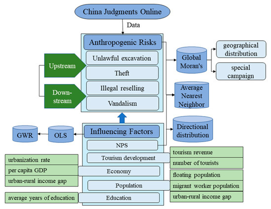
Figure 1.
Research Framework.
3.1. Data Description
The risk data utilized in this paper was obtained from China Judgments Online (https://wenshu.court.gov.cn/ (accessed on 20 June 2022)), an online platform established by the Supreme People’s Court of China in 2013 for disclosing legal judgments. Criminal verdicts related to heritage crimes between 2011 and 2019 were downloaded, and key information, such as time and location, was extracted from the documents. To obtain coordinates for textual addresses, an online conversion tool (https://github.com/sjfkai/mapLocation (accessed on 20 June 2022)) was deployed.
In addition to the general factors that influence risk, such as economic status and population, this study also considers specific factors, namely protected heritage sites and tourism development. The data sources for these factors are described in Table 1.

Table 1.
Data description.
3.1.1. Protected Heritage Sites
Protected heritage sites in this study refer to ancient cultural sites, tombs, buildings, grotto temples, and stone carvings with significant historical, artistic, and scientific values. As an institution established by the state to protect cultural relics through legislation, the sites are categorized into three levels: National Key Protected Heritage Sites (NPS), Provincial-level Protected heritage sites, and County-level Protected heritage sites. Currently, there are 5058 NPS that have been declared as such by the State Council from 1961 to 2019 in eight batches, which can be downloaded from the website of the State Council of China.
Given that the geographical distribution of protected heritage sites may impact crime risks, it was factored into the analysis. Due to the significance and representation of NPS, this paper only analyzes data regarding NPS. Notably, the number of NPS changed only once during the period analyzed in this study, with the sixth batch announced in 2006, the seventh in March 2013, and the eighth in October 2019. The NPS catalog can be downloaded from the Chinese government website (https://www.gov.cn/ (accessed on 20 June 2022)).
3.1.2. Tourism Development
Most NPS in China are open to tourists, and the significant tourist activities occurring at these sites provide ideal cover for criminals seeking to approach their targets. Additionally, sites with a large number of tourists typically enjoy high revenues, making them lucrative targets for theft. This means that cultural relics situated within developed tourist areas may face greater risks than other sites. Unfortunately, the provincial statistical yearbooks do not offer financial expenditure details on tourism industry development. Accordingly, this paper chooses two indicators—tourism revenue and the number of visitors—to reflect the level of tourism development within each province. Both data sources can be found within the provincial statistical yearbooks
3.1.3. Economy
The regional economy may impact the risks of crime in several ways [34,35]. For instance, the economic conditions within a region could directly or indirectly affect the construction of preventative facilities. Within the context of cultural heritage sites, the economy may determine the amount of capital invested in developing security measures around such sites. To capture the economic level of each region quantitatively, three indicators were selected: urbanization rate (urbanization rate refers to the proportion of urban population to the total population.), per capita GDP (per capita GDP is the ratio of GDP to the resident population of a region), and urban–rural income gap (the urban–rural income gap is the ratio of the per capita disposable income of urban households to the per capita disposable income of rural households). These data sources were derived from the statistical yearbooks of the respective provinces.
3.1.4. Population
As economies develop, large numbers of laborers typically move into major cities, leading to high population density and a significant proportion of migrant workers. The Chinese Ministry of Public Security published the National Temporary Resident Statistical Data Collection from 2011 to 2014, covering statistics on the number of migrants in each province. The two indicators of floating population and migrant worker population can be extracted from these books. In addition, population density sourced from statistical yearbooks could represent the population as a third indicator.
3.2. Jenks Natural Breaks Classification
The Jenks Natural Breaks Classification (Jenks) is a popular data classification method widely utilized in Geographic Information Systems (GIS) and is an inherent feature of ArcGIS Pro version 3.0.1. The method was developed in the 1960s, in which Jenks [36,37] posits the presence of breakpoints between data as the basis for classifying them using “natural” divisions. The key principle of this algorithm is cluster analysis, which maximizes between-group variance and minimizes within-group variance.
Firstly, calculate the sum of squared deviations for array mean (SDAM). The mean value is calculated as follows:
The equation for SDAM is:
where is the number of elements in the array; is the value of the i-th element.
Then, iterate through each range combination, calculate the “sum of squared deviations for class means” (SDCM_ALL), and find the minimum of these values, denoted as SDCMmin. The elements are divided into classes, so that the classification result can be divided into subsets, one of which is the case of . Calculate the SDAMi, SDAMj,…, SDAMn for each subset, and sum SDCM1 as:
Similarly, the classification results can also be classified into other cases of class . The value of is calculated successively, and the smallest one of them is selected as the final result SDCMmin, so that the classification range is the best classification.
Finally, the “goodness of variance fit” (GVF) is calculated:
The value of is between 0 and 1, 1 indicates an excellent fit and 0 indicates a very poor fit. The higher the gradient indicates the greater the difference between classes, and the test proves that the classification obtained by the smallest SDCMmin in step (2) has the largest gradient value, which can lead to the conclusion that the results of the natural breaks classification method are desirable.
3.3. Geographical Weighted Regression
The linear regression is the most commonly used model in statistical analysis, while the most basic method is Ordinary Least Squares (OLS) [38]. The idea is to make the following:
where is a set of linearly independent functions selected in advance, is a coefficient to be determined (k = 1, 2…, m, m < n), and the fitting criterion is to make minimize the sum of the squares of the distances from .
There are two basic assumptions of OLS: the errors are random and the model residuals are uncorrelated. However, there is always spatial heterogeneity and spatial autocorrelation in the associations between spatial data, thus violating the principle of using OLS models. Geographical Weighted Regression (GWR) is a local linear regression method based on the modeling of spatially varying relationships [39,40], which generates a regression model describing local relationships at each location in the study area, thus effectively explaining the local spatial relationships and spatial heterogeneity of the variables. The GWR model can generally be expressed as follows:
where is the value of the dependent variable at position ; is the value of the independent variable at position ; are the coordinates of point of the regression analysis; is the intercept term; and are the coefficients of the regression analysis.
3.4. Global Moran’s I
Spatial autocorrelation is a common method for spatial econometric analysis. Its theoretical source is Tobler’s First Law of Geography (TFL), proposed by Waldo Tobler in 1970, that is, “Everything is related to everything else, but near things are more related than distant things” [41]. Spatial autocorrelation can be used to describe the relationship between things in space, that is, to evaluate whether the distribution pattern of a group of elements in space is discrete, an aggregated pattern, or a random pattern. Spatial autocorrelation is generally expressed by Global Moran’s I, and statistical Z-scores and p-values are used to assess the confidence of the results. Moran’s I is an inferential statistic based on the null hypothesis. In the case of the null hypothesis, the distribution between the elements is random. The statistical significance of the p-value and Z-score at this time is the significance of the test results rejecting the null hypothesis. When the p value is not statistically significant, it means that the null hypothesis cannot be rejected, and the elements are randomly distributed in space; when the p value is statistically significant and the Z score is positive, it means that the null hypothesis can be rejected and the elements are more spatially clustered than expected; when the p-value is statistically significant and the Z-score is negative, it indicates that the null hypothesis can be rejected and the features are more spatially dispersed than expected.
Moran’s I was proposed around 1950 [42,43] and can be expressed as:
In the above formula, is the spatial weight of element and and represent the total number of all features. represents a set of all spatial weights, and represents the deviation of from its mean. Among them, is expressed as:
Z-score can be calculated with the following formula:
Global Moran’s I is widely used in crime analysis. For example, in environmental criminology, it is used to compare the degree of clustering of environmental variables with resident variables [44]. Harinam et al. viewed it as a metric that compares the standardized magnitude of difference between the spatial concentration of counted crimes relative to crime severity [45]. This tool also could be used to identify clusters of violent crime during the 3 months of the 2020 COVID-19 lockdown compared to crime rates during an equivalent period [46]. In this paper, the global Moran’s I is used to detect the spatial clustering of heritage crimes and NPS.
4. Results
4.1. Spatial Distribution Pattern Analysis
4.1.1. NPS and Crime Risks
The NPS catalog (see Data collection) was used to extract addresses that were later converted into coordinates. The coordinates were then imported into ArcGIS Pro version 3.0.1, and the Jenks Natural Breaks Classification method (Jenks) was used to classify the number of NPS in China. The analysis reveals that the Shanxi, Henan, and Shaanxi provinces have the highest concentration of NPS. More specifically, the densest distribution is observed in the region where Shanxi borders Henan, followed by the Yangtze River Delta. Throughout its history, China has had many dynasties, with each choosing a city as its capital. As capitals are typically more prosperous than other cities, they tend to leave more cultural heritage behind. The seven ancient capitals of China, which are Xi’an, Luoyang, Nanjing, Beijing, Kaifeng, Hangzhou, and Anyang [47], were chosen due to their superior conditions. Therefore, it is reasonable to suggest that the distribution of NPS is aligned with the division of China’s seven ancient capitals, with Xi’an, Luoyang, Kaifeng, and Anyang located in the provinces of Shanxi, Henan, and Shaanxi.
Additionally, our analysis reveals that the majority of NPS are located in the middle and lower reaches of the Yellow River and the Yangtze River. We further verified this finding by importing a water system map into the software, as shown in Figure 2, where the yellow lines represent the Yangtze River and Yellow River systems, and the blue dots indicate NPS. The distribution of NPS along these two river systems is consistent with archaeological research that highlights multiple foundations of Chinese civilization, with both the Yangtze River and Yellow River being considered the birthplace of this civilization [48]. This paper briefly investigates this phenomenon from two perspectives. First, as the civilizations of the Yellow River and the Yangtze River Basin emerged early, artifacts and relics from these areas are more likely to be preserved over time. Secondly, the natural environment around the rivers is conducive to human life, while water transportation was historically critical for political and economic exchange. Therefore, throughout various dynasties, more people chose to live in these areas and even built their capitals there, resulting in the creation of a wealth of cultural sites.
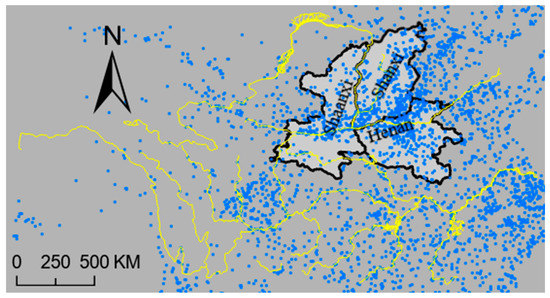
Figure 2.
NPS is mainly distributed in the Yangtze and Yellow River basins.
Moreover, to test the spatial clustering in the distribution of risks and NPS, the Average Nearest Neighbor (ANN) method was employed, which measures the distance between each feature centroid and its nearest neighbor’s centroid location, subsequently obtaining their average value [49,50]. The ANN ratio is given as:
where is the observed mean distance between each feature and its nearest neighbor and is the expected mean distance for the features given in a random pattern. The ANN method takes NPS points or risk points in the space as the inspection objects, calculates the average distance between each observation point and its nearest neighbor, and then compares it with the average distance between two random points. If the former is smaller than the latter, it means that the spatial distribution of the analyzed NPS points or heritage crime points is clustered. In the case of the opposite, it is regarded as decentralized. The ANN index can be expressed as the ratio of the observed average distance to the expected average distance. An ANN of less than 1 corresponds to an aggregated distribution pattern, and an index greater than 1 corresponds to a dispersed distribution pattern [51].
The results of the ANN method are shown in Table 2. It can be found that the ANN of both NPS and risks are less than 1, and the Z scores are less than −2.58, all of which pass the test at a 0.01 significance level and present significant aggregation characteristics.
Table 2.
Analysis results of ANN.
4.1.2. Upstream and Downstream Analysis of Risks
The crime of acquiring cultural objects directly from an unexplored heritage site or NPS is defined in this section as an upstream crime, including unlawful excavation and theft. The re-flow of cultural objects illegally obtained from upstream crime or the resale of cultural objects whose trade is prohibited by law is defined as a downstream crime in this section, including illegal reselling. The crime risk data were organized according to the above classification method, and the classified data were separately used to create hotspot maps (Figure 3) for upstream and downstream crimes in ArcGIS Pro software.
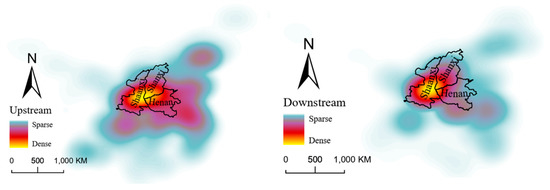
Figure 3.
Heat map of upstream and downstream crimes.
It can be seen that upstream risks are scattered on a large scale in the center and east, and downstream risks are more concentrated, mainly concentrated in the Shaanxi Province. In addition, the Shanxi province also has small-scale hotspots. Therefore, the Shaanxi Province is China’s main hub for combating downstream risks and should continue to intensify its efforts to cut off the chain of cultural heritage risks.
The clustering of downstream risks can be attributed to the fact that illegal reselling typically occurs among acquaintances within the same or neighboring provinces, resulting in relatively small spatial spans. As cultural relics are often advertised and sold online under the false pretenses of being “crafts” or “collectibles,” it requires considerable professional knowledge to authenticate their authenticity. This has made distinguishing cultural relics more challenging and fueled greater volumes of reselling.
To ascertain whether online sales of artifacts have affected the spatial distribution of downstream heritage crimes, we applied the ANN method to analyze the historical heritage crime sites from 2011 to 2019, as detailed in Table 3. The Nearest Neighbor Index did not exhibit an increasing or decreasing trend over the years but instead exhibited a steady cycle of “increasing and then decreasing.” Therefore, it can be deduced that, at this stage, online transactions have yet to present a decisive impact on the geographic pattern of heritage crimes, implying that downstream heritage crimes primarily occur offline.
Table 3.
Analysis of heritage crime sites for each year from 2011 to 2019 using ANN methodology.
4.2. Analysis of Influencing Factors
The distribution of crime risk can be influenced by several factors, including the presence of NPS (as discussed earlier), as well as economic, population, and tourism development. In this section, we treat risks as the dependent variable and these four categories of factors as explanatory variables. To examine their spatial relationships, we performed a spatial regression analysis using the GIS software. Specifically, we used the exploratory regression tool to test the indicators and then applied the Ordinary Least Squares (OLS) method for regression analysis. Based on the results obtained from the OLS analysis, the Geographical Weighted Regression (GWR) model was chosen to examine the spatial heterogeneity of risk.
Taking into account the data availability of the indicators (the data of floating population and migrant workers are only available from 2011 to 2014), and regarding the uniformity of the time, 2011, 2014, and 2019 were selected as the samples for analysis. The exploratory regression tool can evaluate all possible combinations of input explanatory variables and rank the results in reverse order of AdjR2 (adjusted R-squared). The combination with a larger AdjR2 value and fewer explanatory variables is regarded as the optimal combination, and the final results are shown in Table 4. Most of the AdjR2 values are less than 0.5. Only the AdjR2 value for the illegal reselling in 2019 is 0.6, and its corresponding explanatory variable combinations are NPS, urban–rural income gap, and population density. The AdjR2 value for unlawful excavation in 2011 is 0.53, and the corresponding explanatory variable combinations were NPS, the number of domestic tourists, and domestic tourism income. In the next step, the OLS analysis was only carried out on the risk of unlawful excavation in 2011 and illegal reselling in 2019. The results are shown in Table 5, and the diagnosis results are shown in Table 6. From the results, it can be concluded that:
Table 4.
Exploratory regression tool output for indicators.
Table 5.
The output of the OLS method.
Table 6.
OLS diagnostic report.
(1) VIF in Table 5 represents the variance inflation factor (VIF), and if VIF is less than 3, it means there is no multicollinearity problem between variables. Only “illegal reselling in 2019” can pass the test.
(2) The Koenker (BP) statistic in Table 6 indicates whether the relationship between the dependent variable and the explanatory variable is stable. The Koenker (BP) for the two risks listed in the table is significant, indicating that both types of data are not stationary. In this case, the Robust_Pr (robustness indicator of probability) in Table 6 needs to be considered rather than the p value. In 2011, the Robust_Pr of all independent variables of unlawful excavation was less than 0.05. The Robust_Pr value of NPS and population density of illegal reselling in 2019 was less than 0.05, while the value of the urban–rural income gap was greater than 0.05, which shows that the urban–rural income gap index is not helpful for the regression model. On the other hand, the significant Koenker (BP) value also means that the two risks can be further analyzed by the GWR model to verify their spatial heterogeneity as follows:
(3) When the Koenker (BP) value is significant, if the joint chi-square statistic is also significant, the model is significant.
(4) The Jarque–Bera statistic in Table 6 indicates whether the residuals of the model conform to a normal distribution. The Jarque–Bera statistic of unlawful excavation in 2011 in the table is significant, indicating that the model is biased and key explanatory variables are missing. The Jarque–Bera statistic for illegal reselling in 2019 is not significant, indicating that the model meets the needs. Therefore, only illegal reselling in 2019 was allowed for the next step of GWR analysis to compare the performance of OLS and GWR.
(5) The performance of the model was tested by R-squared, adjusted R-squared, and Akaike information criterion (AICc). R-squared or adjusted R-squared indicated the goodness of fit of the model. The goodness of fit of the two risks was between 0.5 and 0.6, and the overall performance of the model was average. The goodness of fit of the illegal reselling in 2019 was slightly better than that of the unlawful excavation in 2011. The AICc value is often used to compare the performance between models. The smaller the AICc value, the better the model performance. Generally, a difference of more than 3 indicates that the improved model is better than the original model. In the next step, this indicator was be used to compare the model performance of OLS and GWR.
(6) The linear equation of the illegal reselling in 2019 can be expressed as:
To test the spatial heterogeneity of illegal reselling in 2019, this risk was used as the dependent variable, NPS and population density were used as explanatory variables, and the model type was selected as a continuous (Gaussian) for GWR analysis. The R-squared value of the GWR model was 0.6108, and the adjusted R-squared value was 0.4899, both lower than the OLS model. The AICc value was 184.4841, which is larger than the value under OLS of 173.521, so the overall performance of the GWR model was lower than that of the OLS model, and there was no spatial heterogeneity in illegal reselling in 2019.
After conducting OLS and GWR analysis of crime risks, the following conclusions can be drawn:
(1) Regarding the economic conditions, the three indicators of urbanization rate, per capita GDP, and urban–rural income gap did not have a significant impact on crime risks. One possible explanation is that provinces with good economies may not have allocated sufficient funds for security facility construction. Another explanation could be that, while provinces with good economies may have invested more in security facility construction, there are issues with system usage or the daily management of NPS. Further field research is recommended to determine appropriate measures for enhancing the security of cultural relics.
(2) Among population factors, the floating population and migrant workers had no impact on crime risks; only population density had an impact on illegal reselling in 2019. In China, migrants are typically defined as individuals residing in a location for six months or longer. However, since criminals do not usually remain near heritage sites for extended periods, this indicator cannot properly reflect their movements. Moreover, higher incidences of illegal reselling occurred in provinces with higher population densities.
(3) Regarding NPS, both unlawful excavation in 2011 and illegal reselling in 2019 were impacted by them, demonstrating that even the highest level of protected NPS faces a significant risk of being illegally excavated. This highlights the enormous historical and cultural value of these items, as well as their high economic worth. Heritage criminals eagerly target such NPS sites for profit.
(4) Tourism development had an influence on unlawful excavation in 2011. Many of China’s NPSs are tourist attractions, and a booming tourism industry can mean more protected heritage sites in a province, increasing the risk of crimes occurring in accordance with the analysis in the previous paragraph.
4.3. The Global Moran’s I Analysis of Crime Risks
This section describes the calculation of the Global Moran’s I of four crime risks and NPS and summarizes the distribution of cultural heritage risks among provinces. Firstly, to reduce the error of spatial calculation, the coordinate system was also spatially projected. Secondly, the total number of crime risk events for the period of 2011–2019 was calculated, and the data, along with the eighth batch of NPS data, was imported into the projected coordinate system, with the conceptualization of the spatial relationship choosing “adjacent edge corners.” The results are shown in Table 7. It can be seen that the p values of NPS and the four risks are all less than 0.05, and the Z scores are all greater than 1.96, so their distributions all have significant clustering characteristics. Among them, unlawful excavation is the most concentrated.
Table 7.
The Global Moran’s I of four crime risks and NPS.
In the next step, the sum of the four risks for each year were calculated and expressed. Ten sets of results are shown in Table 8, which were obtained by calculating Global Moran’s I for each year. The Z-scores and p-values show that each group presented a significant aggregation state. To further observe the geographical distribution trend, a line graph was made out of the Global Moran’s I values (Figure 4).
Table 8.
Global Moran’s I of crime risk.
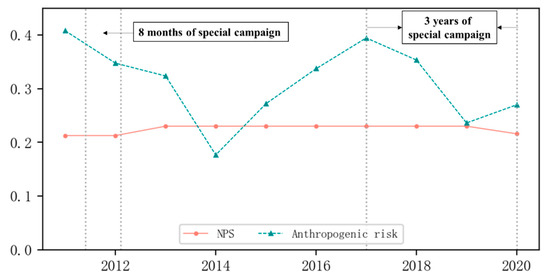
Figure 4.
Global Moran’s I line graph of crime risk from 2011 to 2019.
Figure 4 indicates that the Global Moran’s I of NPS has remained relatively stable over time, with only minor fluctuations despite an increase by 1943 in the number of NPS announced in the seventh batch in March 2013. At this point, the Global Moran’s I increased further, indicating stronger clustering. This illustrates that the additional NPS listings originated mostly from provinces possessing significant cultural relics that border each other geographically. Conversely, the Global Moran’s I for crime risk was more volatile, declining since 2011, with a notable trough occurring in 2014. In the same year, there was also a shift in p-value significance level, changing from 0.01 to 0.05, followed by a continuous increase in Global Moran’s I. After peaking in 2017, it began to decrease again, and a second trough emerged in 2019.
The appearance of these trends stems from China’s specific campaign against heritage crimes. Typically, after significant police operations are concluded in China, updates are released via the official website (www.mps.gov.cn (accessed on 20 June 2022)) of the Ministry of Public Security (MPS). These releases can be used to deduce the anti-crime actions taken by individual provinces at a macroscopic level. As previously analyzed, heritage crimes tend to happen in contiguous regions, such as the Shaanxi-Shanxi-Henan Province region, the Yangtze River Delta region, etc. Therefore, provinces rich in cultural relics and sharing borders are susceptible to clustering characteristics, contributing to the sustained elevation of the Global Moran’s I for crime risks.
According to MPS’s official website, China’s first special campaign against heritage crimes was conducted from December 2009 to June 2010, covering only nine key provinces. In May 2011, an eight-month long campaign was launched again, expanding the scope to seventeen key areas. As the number of provinces involved increased, crime risks were more evenly distributed across the country, leading to the sustained decline of Global Moran’s I until 2014. Another downward trend appeared after 2017, when the MPS and State Administration of Cultural Heritage jointly initiated a three-year-long nationwide campaign. During these campaigns, each province took actions to combat heritage crimes, offsetting the clustering characteristics of some heritage-rich and border-connected regions.
However, between 2015 and 2017, no national-level special campaigns were held. News reports indicate that provinces with significant cultural relics continue to conduct their own special campaigns in recent years. For instance, Shanxi launched a hundred-day operation to combat heritage crimes in 2015, while the Shaanxi Province implemented the “Eagle” special campaign. This phenomenon can be attributed to two factors. Firstly, provinces with abundant cultural relics may experience more heritage crimes. Secondly, these provinces gain more experience in resolving heritage crimes, leading to the reporting of more news and case-solving activities. When provinces with adjacent borders and rich cultural relic resources see significantly more criminal cases than others, they will again exhibit clustering.
5. Discussion
Preventing crime risks has both contemporary and future merits. By utilizing methods such as spatial analysis, correlation analysis, and spatial econometrics, this paper provides in-depth insights into the geographical distribution patterns, influencing factors, and policy sensitivities of crime risks. The results suggest that, when establishing security systems for protected heritage sites, their spatial characteristics, impact of tourism and economy, and potential policy effects on heritage crime risk should all be taken into account. Meanwhile, national or local governments should formulate heritage conservation policies based on fine-grained data and thorough analysis at the micro level. Targeted policies are needed for NPS in different spatial environments with varying economic and tourism conditions.
To circumvent the lack of crime risk data for cultural relics, this paper pioneers an approach of obtaining crime data from public judgment documents, which may have broader applications in the acquisition of other crime data.
In analyzing the influencing factors of heritage crime, crime is seen as a complex social phenomenon, and there are many factors that influence crime. Heritage managers should consider variables such as staff capacity, visitor limits, and heritage ontology alongside crime risk reduction when assessing the impact of tourism on heritage crime. While migrant workers are often assumed to be the main perpetrators of heritage crime, identifying them can require a much longer policy period than the time frame for detecting heritage crime trends. Impact factor analysis can thus provide useful indicators for detecting macro-level crime trends.
Criminal policy, particularly for non-traditional types of crime such as heritage crime, can also significantly impact crime distribution. Therefore, legislative safeguards against heritage crime should be strengthened if policy is found to substantially affect crime distribution.
While limited by the quality of crime risk data and available spatial analysis techniques, this paper highlights current crime risk patterns and emphasizes the need to enhance heritage security facilities and prioritize the protection of precious historical heritage.
6. Conclusions
Based on the crime risk data obtained from the Judgment Document Online, this paper used the ANN method, Directional Distribution (Standard Deviational Ellipse), OLS, GWR, and Global Moran’s I methods to explore and summarize the spatial characteristics of crime risks. The main conclusions are as follows:
Both NPS and crime risks showed clustering distribution characteristics in space. Most of the hot spots were located in the middle and lower reaches of the Yangtze River and the Yellow River, and the directional distribution showed different characteristics. Cases of cultural heritage crime involving illegal reselling typically remain within the province where the offence took place or nearby regions, with little spatial dispersion. However, the emergence of online reselling in recent years has made the flow of cultural heritages more scattered. The economy does not have an impact on crime risks. Specific types of crime risks are influenced by factors such as population density, distribution of NPS, and tourism development, while crime risk itself does not exhibit significant spatial heterogeneity. The agglomeration of crime risks in the time scale analyzed is related to China’s special campaign against heritage crime, and Global Moran’s I declined when a nationwide campaign was launched.
Extensive research has been conducted on the quantitative analysis of crime, and its findings have significantly informed practical police work, with their efficacy in crime control now being widely acknowledged. However, there has been limited quantitative research in the subdivision of heritage crime risk, and developing a systematic theory of heritage crime control requires a great deal of work. In-depth research on heritage crime is particularly significant, as it not only helps maintain the stability of the social environment but also protects precious historical and cultural heritage, as well as substantial economic interests. Therefore, conducting quantitative criminological research on heritage conservation and applying the findings to the practical work of heritage conservation is crucial. Utilizing a range of time–space criminological theories can support law enforcement efforts, and practical experience in combating heritage crime can also contribute to generating new criminological theories.
Author Contributions
Yiming Zhai and Ning Ding conceived and designed the study and wrote the manuscript. Yiming Zhai and Hongyu Lv analyzed the results. Ning Ding provided key suggestions and helped with the writing of the manuscript. All authors have read and agreed to the published version of the manuscript.
Funding
This research was funded by the National Key R&D Program of China (No. 2020YFC1522600) and the Basic Research Foundation of People’s Public Security University of China (2022JKF02010).
Data Availability Statement
The data that support the findings of this study are available from the China Judgments Online (https://wenshu.court.gov.cn/ (accessed on 20 June 2022)) and the Chinese government website (https://www.gov.cn/ (accessed on 20 June 2022)).
Acknowledgments
We thank the anonymous reviewers and academic editor for the constructive suggestions and insightful comments that substantially improved the quality of this research.
Conflicts of Interest
The authors declare no conflict of interest.
References
- Grove, L. Heritocide? Defining and Exploring Heritage Crime. Public. Archaeol. 2013, 12, 242–254. [Google Scholar] [CrossRef]
- Grove, L.; Thomas, S. (Eds.) Heritage Crime; Palgrave Macmillan: London, UK, 2014; ISBN 978-1-349-47078-5. [Google Scholar]
- Charney, N. (Ed.) Art Crime: Terrorists, Tomb Raiders, Forgers and Thieves; Palgrave Macmillan: London, UK, 2016; ISBN 978-1-349-55370-9. [Google Scholar]
- Maio, R.; Ferreira, T.M.; Vicente, R. A Critical Discussion on the Earthquake Risk Mitigation of Urban Cultural Heritage Assets. Int. J. Disast. Risk Re. 2018, 27, 239–247. [Google Scholar] [CrossRef]
- Wang, J.-J. Flood Risk Maps to Cultural Heritage: Measures and Process. J. Cult. Herit. 2014, 16, 210–220. [Google Scholar] [CrossRef]
- Wu, P.-S.; Hsieh, C.-M.; Hsu, M.-F. Using Heritage Risk Maps as an Approach to Estimating the Threat to Materials of Traditional Buildings in Tainan (Taiwan). J. Cult. Herit. 2014, 15, 441–447. [Google Scholar] [CrossRef]
- Kim, H.; Matuszka, T.; Kim, J.-I.; Kim, J.; Woo, W. Ontology-Based Mobile Augmented Reality in Cultural Heritage Sites: Information Modeling and User Study. Multimed. Tools Appl. 2017, 76, 26001–26029. [Google Scholar] [CrossRef]
- Zhao, J.; Wen, R.; Mei, W. Systematic Method for Monitoring and Early-Warning of Garden Heritage Ontology Used in the Suzhou Classical Garden Heritage. J. Environ. Eng. Landsc. 2020, 28, 157–173. [Google Scholar] [CrossRef]
- Novotny, Á.; Dávid, L.; Csáfor, H. Applying RFID Technology in the Retail Industry—Benefits and Concerns from the Consumer’s Perspective. Amfiteatru Econ. J. 2015, 17, 615–631. [Google Scholar]
- Çınar, K. Role of Mobile Technology for Tourism Development. In The Emerald Handbook of ICT in Tourism and Hospitality; Hassan, A., Sharma, A., Eds.; Emerald Publishing Limited: Bingley, UK, 2020; pp. 273–288. ISBN 978-1-83982-689-4. [Google Scholar]
- Appiotti, F.; Assumma, V.; Bottero, M.; Campostrini, P.; Datola, G.; Lombardi, P.; Rinaldi, E. Definition of a Risk Assessment Model within a European Interoperable Database Platform (EID) for Cultural Heritage. J. Cult. Herit. 2020, 46, 268–277. [Google Scholar] [CrossRef]
- Grove, L.; Thomas, S.; Daubney, A. Fool’s Gold? A Critical Assessment of Sources of Data on Heritage Crime. Disaster Prev. Manag. Int. J. 2018, 29, 10–21. [Google Scholar] [CrossRef]
- Habib, U.; Areeba, U.; Sarfraz, S.; Ahmad, M.; Ullah, M.; Mazzara, M. Spatiotemporal Analysis of Web News Archives for Crime Prediction. Appl. Sci. 2020, 10, 8220. [Google Scholar] [CrossRef]
- Li, J.; Chen, Y.; Yao, X.; Chen, A. Risk Management Priority Assessment of Heritage Sites in China Based on Entropy Weight and TOPSIS. J. Cult. Herit. 2021, 49, 10–18. [Google Scholar] [CrossRef]
- Oosterman, N.; Yates, D. (Eds.) Studies in art, heritage, law and the market. In Crime and Art: Sociological and Criminological Perspectives of Crimes in the Art World; Springer: Cham, Switzerland, 2021; ISBN 978-3-030-84856-9. [Google Scholar]
- Figueiredo, R.; Romão, X.; Paupério, E. Flood Risk Assessment of Cultural Heritage at Large Spatial Scales: Framework and Application to Mainland Portugal. J. Cult. Herit. 2020, 43, 163–174. [Google Scholar] [CrossRef]
- Mallinis, G.; Mitsopoulos, I.; Beltran, E.; Goldammer, J. Assessing Wildfire Risk in Cultural Heritage Properties Using High Spatial and Temporal Resolution Satellite Imagery and Spatially Explicit Fire Simulations: The Case of Holy Mount Athos, Greece. Forests 2016, 7, 46. [Google Scholar] [CrossRef]
- Lombardo, L.; Tanyas, H.; Nicu, I.C. Spatial Modeling of Multi-Hazard Threat to Cultural Heritage Sites. Eng. Geol. 2020, 277, 105776. [Google Scholar] [CrossRef]
- Cerra, D.; Plank, S.; Lysandrou, V.; Tian, J. Cultural Heritage Sites in Danger—Towards Automatic Damage Detection from Space. Remote Sens. 2016, 8, 781. [Google Scholar] [CrossRef]
- Xie, Y.; Yang, R.; Liang, Y.; Li, W.; Chen, F. The Spatial Relationship and Evolution of World Cultural Heritage Sites and Neighbouring Towns. Remote Sens. 2022, 14, 4724. [Google Scholar] [CrossRef]
- Elfadaly, A.; Attia, W.; Qelichi, M.M.; Murgante, B.; Lasaponara, R. Management of Cultural Heritage Sites Using Remote Sensing Indices and Spatial Analysis Techniques. Surv. Geophys. 2018, 39, 1347–1377. [Google Scholar] [CrossRef]
- Yao, Y.; Wang, X.; Lu, L.; Liu, C.; Wu, Q.; Ren, H.; Yang, S.; Sun, R.; Luo, L.; Wu, K. Proportionated Distributions in Spatiotemporal Structure of the World Cultural Heritage Sites: Analysis and Countermeasures. Sustainability 2021, 13, 2148. [Google Scholar] [CrossRef]
- Valagussa, A.; Frattini, P.; Crosta, G.; Spizzichino, D.; Leoni, G.; Margottini, C. Multi-Risk Analysis on European Cultural and Natural UNESCO Heritage Sites. Nat. Hazards 2021, 105, 2659–2676. [Google Scholar] [CrossRef]
- Nebbia, M.; Cilio, F.; Bobomulloev, B. Spatial Risk Assessment and the Protection of Cultural Heritage in Southern Tajikistan. J. Cult. Herit. 2021, 49, 183–196. [Google Scholar] [CrossRef]
- Ranson, M. Crime, Weather, and Climate Change. J. Environ. Econ. Manag. 2014, 67, 274–302. [Google Scholar] [CrossRef]
- Peng, C.; Xueming, S.; Hongyong, Y.; Dengsheng, L. Assessing Temporal and Weather Influences on Property Crime in Beijing, China. Crime Law Soc. Chang. 2011, 55, 1–13. [Google Scholar] [CrossRef]
- Hu, X.; Chen, P.; Huang, H.; Sun, T.; Li, D. Contrasting Impacts of Heat Stress on Violent and Nonviolent Robbery in Beijing, China. Nat. Hazards 2017, 87, 961–972. [Google Scholar] [CrossRef]
- Algahtany, M.; Kumar, L.; Barclay, E. A Tested Method for Assessing and Predicting Weather-Crime Associations. Environ. Sci. Pollut. R. 2022, 29, 75013–75030. [Google Scholar] [CrossRef]
- Ding, N.; Zhai, Y. Crime Prevention of Bus Pickpocketing in Beijing, China: Does Air Quality Affect Crime? Secur. J. 2019, 34, 262–277. [Google Scholar] [CrossRef]
- Zhou, H.; Liu, L.; Lan, M.; Yang, B.; Wang, Z. Assessing the Impact of Nightlight Gradients on Street Robbery and Burglary in Cincinnati of Ohio State, USA. Remote Sens. 2019, 11, 1958. [Google Scholar] [CrossRef]
- Yue, H.; Zhu, X.; Ye, X.; Guo, W. The Local Colocation Patterns of Crime and Land-Use Features in Wuhan, China. ISPRS Int. J. Geo-Inf. 2017, 6, 307. [Google Scholar] [CrossRef]
- Ristea, A.; Kurland, J.; Resch, B.; Leitner, M.; Langford, C. Estimating the Spatial Distribution of Crime Events around a Football Stadium from Georeferenced Tweets. ISPRS Int. J. Geo-Inf. 2018, 7, 43. [Google Scholar] [CrossRef]
- Chen, P.; Kurland, J.; Piquero, A.R.; Borrion, H. Measuring the Impact of the COVID-19 Lockdown on Crime in a Medium-Sized City in China. J. Exp. Criminol. 2021. [Google Scholar] [CrossRef]
- Rosenfeld, R.; Fornango, R. The Impact of Economic Conditions on Robbery and Property Crime: The Role of Consumer Sentiment. Criminology 2008, 45, 735–769. [Google Scholar] [CrossRef]
- Detotto, C.; Otranto, E. Cycles in Crime and Economy: Leading, Lagging and Coincident Behaviors. J. Quant. Criminol. 2012, 28, 295–317. [Google Scholar] [CrossRef]
- Jenks, G.F. Generalization In Statistical Mapping. Ann. Assoc. Am. Geogr. 1963, 53, 15–26. [Google Scholar] [CrossRef]
- Jenks, G.F. The Data Model Concept in Statistical Mapping; C. Bertelsmann: Gütersloh, Germany, 1967. [Google Scholar]
- Dempster, A.P.; Schatzoff, M.; Wermuth, N. A Simulation Study of Alternatives to Ordinary Least Squares. J. Am. Stat. Assoc. 1977, 72, 77–91. [Google Scholar] [CrossRef]
- Fotheringham, A.S.; Brunsdon, C.; Charlton, M. Geographically Weighted Regression: The Analysis of Spatially Varying Relationships; Wiley: Chichester, UK; Hoboken, NJ, USA, 2002; ISBN 978-0-471-49616-8. [Google Scholar]
- Brunsdon, C.; Fotheringham, A.S.; Charlton, M.E. Geographically Weighted Regression: A Method for Exploring Spatial Nonstationarity. Geogr. Anal. 2010, 28, 281–298. [Google Scholar] [CrossRef]
- Tobler, W.R. A Computer Movie Simulating Urban Growth in the Detroit Region. Econ. Geogr. 1970, 46, 234–240. [Google Scholar] [CrossRef]
- Moran, P.A.P. Notes on Continuous Stochastic Phenomena. Biometrika 1950, 37, 17–23. [Google Scholar] [CrossRef]
- Moran, P.A.P. The Interpretation of Statistical Maps. J. R. Stat. Soc. Ser. B (Methodol.) 1948, 10, 243–251. [Google Scholar] [CrossRef]
- Andresen, M.A. The Ambient Population and Crime Analysis. Prof. Geogr. 2011, 63, 193–212. [Google Scholar] [CrossRef]
- Harinam, V.; Bavcevic, Z.; Ariel, B. Spatial Distribution and Developmental Trajectories of Crime versus Crime Severity: Do Not Abandon the Count-Based Model Just Yet. Crime. Sci. 2022, 11, 14. [Google Scholar] [CrossRef]
- Moise, I.K.; Piquero, A.R. Geographic Disparities in Violent Crime during the COVID-19 Lockdown in Miami-Dade County, Florida, 2018–2020. J. Exp. Criminol. 2023, 19, 97–106. [Google Scholar] [CrossRef]
- Chen, Q. China’s Seven Ancient Capitals; China Youth Press: Beijing, China, 2005; ISBN 978-7-5006-0727-4. [Google Scholar]
- Chen, L. On the Origin of the Chinese Civilization and the Chief Characteristics of Its Early Stage Development. J. Cent. Univ. Natl. 2000, 27, 22–34. [Google Scholar] [CrossRef]
- Ebdon, D. Statistics in Geography, 2nd ed.; Rev. with 17 Programs; B. Blackwell: Oxford, UK; New York, NY, USA, 1985; ISBN 978-0-631-13688-0. [Google Scholar]
- Vidal Ruiz, E. An Algorithm for Finding Nearest Neighbours in (Approximately) Constant Average Time. Pattern Recognit. Lett. 1986, 4, 145–157. [Google Scholar] [CrossRef]
- Amissah, M.B.; Wemegah, T.D.; Okyere, F.T. Crime Mapping and Analysis in the Dansoman Police Subdivision, Accra, Ghana—A Geographic Information Systems Approach. J. Environ. Earth Sci. 2014, 4, 28–37. [Google Scholar]


Disclaimer/Publisher’s Note: The statements, opinions and data contained in all publications are solely those of the individual author(s) and contributor(s) and not of MDPI and/or the editor(s). MDPI and/or the editor(s) disclaim responsibility for any injury to people or property resulting from any ideas, methods, instructions or products referred to in the content. |
© 2023 by the authors. Licensee MDPI, Basel, Switzerland. This article is an open access article distributed under the terms and conditions of the Creative Commons Attribution (CC BY) license (https://creativecommons.org/licenses/by/4.0/).