Convolutional Neural Network-Based Deep Learning Approach for Automatic Flood Mapping Using NovaSAR-1 and Sentinel-1 Data

Abstract

The accuracy of most SAR-based flood classification and segmentation derived from semi-automated algorithms is often limited due to complicated radar backscatter. However, deep learning techniques, now widely applied in image classifications, have demonstrated excellent potential for mapping complex scenes and improving flood mapping accuracy. Therefore, this study aims to compare the image classification accuracy of three convolutional neural network (CNN)-based encoder–decoders (i.e., U-Net, PSPNet and DeepLapV3) by leveraging the end-to-end ArcGIS Pro workflow. A specific objective of this method consists of labelling and training each CNN model separately on publicly available dual-polarised pre-flood data (i.e., Sentinel-1 and NovaSAR-1) based on the ResNet convolutional backbone via a transfer learning approach. The neural network results were evaluated using multiple model training trials, validation loss, training loss and confusion matrix from test datasets. During testing on the post-flood data, the results revealed that U-Net marginally outperformed the other models. In this study, the overall accuracy and F1-score reached 99% and 98% on the test data, respectively. Interestingly, the segmentation results showed less use of manual cleaning, thus encouraging the use of open-source image data for the rapid, accurate and continuous monitoring of floods using the CNN-based approach.

1. Introduction

Floods are among the most frequent and devastating natural disasters in the world today, and floods have accounted for the large-scale destruction of property and loss of human life [1,2]. In most cases, floods are associated with long-lasting periods of cloud cover when heavy rainfall occurs [3]. However, during these events, the accessibility to accurate information is often limited, and a cost- and time-efficient approach that is crucial for situation awareness, the allocation of resources and emergency response operations is generally lacking [4].

Remote sensing techniques have been proven to provide valuable information for monitoring and rescue operations in the event of floods in a time- and cost-efficient manner due to their synoptic view [4]. The synthetic aperture radar (SAR) is one of the most used satellite-based systems in recent years due to the increased availability of high spatio-temporal resolution imagery, its frequent revisit capability and its ability to capture data from targets on the earth’s surface in nearly all weather conditions and during any time of the day [5,6,7,8]. A SAR sensor not only offers advantages in all weather conditions but also enables shape distinctions between water and land [9,10,11].

In SAR imagery, the detection and extraction of water pixels is a measure of its distinctive radar signature. However, the side-viewing geometry and the sensitivity of the microwaves to surface roughness often complicate the radar backscatter response during flood detection [12,13,14]. Calm water produces a smooth surface, which is often in a dark tone, indicating low backscatters on SAR images [4]. In contrast, rough water appears brighter on SAR imagery than calm water as it reflects signals in different directions [15]. Oftentimes during flooding, the variability of different environmental conditions such as topography, shadows and wind can adversely complicate the radar backscatter response, which creates some challenges in establishing the optimal threshold values to map the extent of a flooded area.

In built-up areas for instance, the double-bounce effect has been observed due to the presence of buildings, hence leading to the application of several analytical methods to address this [16,17,18,19]. For instance, ref. [16] used SAR interferometry coherence and intensity to map floodwater in urban and agricultural areas via thresholding, region growing and change detection methods. The combination of these methods achieved compelling results as a multitemporal coherence trend was seen to compliment SAR intensity, thus reducing misclassification errors. Similarly, ref. [17] performed urban flood mapping from a very high-resolution TerraSAR-X via a hybrid method comprising radiometric thresholding, region growing and change detection. The results revealed that the methods can achieve a satisfactory outcome in mapping challenging situations. In another urban flood mapping study, ref. [18] used an unsupervised Bayesian network fusion framework for SAR intensity and interferometric coherence. According to the study, the fusion of the coherence and the intensity image can account for flood uncertainty and provide valuable information for urban flood mapping. In addition, the authors of [19] demonstrated the use of a Sentinel-1 based SAR coherence to detect floodwater in urban areas. Using an automatic algorithm, the study leveraged the Sentinel-1 short temporal and perpendicular baselines, in which the evaluation compared well with Digital Global crowdsourcing and the FEMA hydrological models during a cross-comparison.

In rural areas, vegetation cover causes ambiguity in SAR radar signature’s ability to accurately detect the presence of flood [20,21]. However, a common way to identify a flooded area under vegetation cover is largely dependent on the intensity of the radar signature from the flooded vegetation compared to a non-flooded area due to double-bounce effects [22].

For many years, the thresholding method has been used in SAR-based flood detection and is usually categorised into flooded and not flooded areas in SAR images. To perform floodwater extraction, a threshold value is assigned such that a pixel with a radar backscatter lower than the assigned value is classified as flood [16,17]. This method is computationally efficient and can be applied in real time. However, a notable shortcoming with thresholding is the mapping of areas with similar low radar backscatter as not all pixels with low radar backscatter are covered with water. Overall, some studies have established that there is no universal threshold value for water backscatter [4]. One way to overcome this is using an InSAR change detection approach to map floodwater in urban and vegetated areas [16]. However, even though this approach is effective, image segmentation and classification require necessary ancillary data, which may not be readily available.

Similarly, region growing is one method that has been used in many studies for homogeneous flood mapping. In this method based on seed pixels, adjacent pixels within a whole SAR are connected to seed pixels belonging to the seed region. This iterative process stops when conditions are met, and then the seed pixels are classified as water. Creating accurate seed pixels manually can be challenging and time-consuming. To address this limitation, the selection of seed pixels can be performed automatically using the thresholding method. Overall, these techniques are still faced with the inherent limitations of thresholding methods [14,15].

As noted in several studies, these methods have achieved some successful results but not without some limitations. Firstly, due to the sensitivity of these models to the presence of speckle noise in SAR images, pre-processing filters are applied; however, these filters can also cause information loss, thus affecting the overall performance of these techniques. Additionally, most of these models need some careful human interventions to manually update training parameters and require high accuracy DEM and ancillary data from different sources, which are not readily available, to achieve optimal results. It intuitively follows that during human intervention, errors and bias may be introduced in overall data management. A major disadvantage of these methods is the loss of time in producing maps, especially for the activation of an emergency response in the event of flood disasters [4,23].

To address this knowledge gap, machine learning techniques have increasingly been applied to a wide range of Earth observation studies due to the increasingly large amount of data that are being collected and the timely image processing required [24,25]. Some studies revealed that the emergence of deep learning can automate image processing and compare well with human performance or even achieve superior results [26,27]. These techniques have proven to provide solutions that generalise varying complex and dynamic environmental settings [23,27,28,29,30]. In recent years, machine learning, a purely data-driven technique, has been used to extract water pixels, with most focusing on flood mapping and monitoring.

Various techniques have been applied to automate the mapping of flood extent. In recent years, a common way has been the use of machine learning-based techniques on imagery collected from optical and multispectral sensors, which is often a fusion of multiple datasets [31,32,33,34,35]. While passive sensors have shown great promise, they are still limited to a time interval and restricted to weather conditions such as cloud cover, thus making them less suited for emergency response operations in the event of floods. Due to the increased availability of high spatio-temporal resolution imagery from SAR sensors and their ability to capture data from Earth’s surface in all weather conditions, the use of machine learning techniques for SAR-based flood detection has continued to improve. Some notable studies include the use of Sentinel-1 imagery and machine learning for the supervised and unsupervised flood image classification of the City of San Diego, CA, USA [36]. The study applied machine learning random forest (RF), support vector machine (SVM) and maximum likelihood classifier and developed a new unsupervised framework that was combined with the Otsu algorithm, fuzzy rules and iso-clustering [36]. The analysis of the results obtained from this study showed that this approach can provide a more robust and time-efficient solution for the mapping and risk management of flooded transportation facilities [36]. Another method tested for flood mapping was the use of the Gaussian mixture model [37]. The convolutional neural network (CNN), a deep learning neural network, is now becoming one of the most frequently used machine learning pixel-based segmentation techniques [4]. This automatic processing chain was tested on multiple sites and was found to be efficient in extracting flood and surface waters automatically using smooth labelling on Sentinel-1 data [37] The huge computational requirements for the analyses and interpretation of large datasets make it of great interest to researchers, even though it has not been widely explored [38]. It has the capability of multiple high levels of generalisation in the extraction of complex spatial features [27,39]. Moreover, it is a scalable technique that allows the increase in and management of large datasets with increasing performance [40,41].

CNNs have been used in several studies for the classification of land cover and groundwater potential zones, polarimetric SAR landcover classification [42], crop classification [43] and urban growth [44]. However, more recently, there have been different CNN techniques applied to the detection of various scenarios of water bodies and flood events globally. Wu, Yang and Wang [45] used an SAR-based multi-depth flood detection convolutional neural network (MDFD-CNN) for water region classification and extraction in a complex environment. The MDFD-CNN achieved a more robust result compared to traditional methods. In addition, Li et al. [16] introduced and experimented on the multi-temporal SAR-data-derived self-learning convolutional neural network (A-SL CNN) to reduce the impact of limited annotated training samples. The achieved result has shown that the proposed ASL-CNN outperformed its supervised counterpart.

Similarly, Nemni et al. [4] designed a Sentinel-1 -based fully convolution neural network (CNN) for flood pixels extraction. The methodology was found to speed up the development of flood maps by 80%, as well as obtain strong performance metrics over the selected locations with varying environmental conditions [4]. Furthermore, Wu et al. [46] used dual-polarised SAR images based on multi-scale DeepLab model for flood detection. The study proposed a CNN-based MS-DeepLab model and other models, (i.e., PSPNet, U-Net and DeeLabV3) with the MobileNetV2 convolutional backbone. The results showed that the MS-DeepLab model successfully improved the feature extraction ability, especially for boundary detection, and was the best performing model in the study [46].

Furthermore, Zhao et al. [30] used a CNN deep learning-based model for flood detection in Xinxiang, China. The authors successfully developed and implemented the U-Net-based model for water body extraction with Gaofen-3 (GF3) SAR data, which showed strong model performance in water extraction. Compared to the standard U-Net structure, an attention mechanism was integrated into the encoding part of the neural network to improve the accuracy and efficiency of the water extraction [30]. As shown in these studies, the application of convolutional neural networks has the potential to revolutionise the development of flood maps given their high classification accuracy over traditional methods. In another study, Katiyar, Tamkuan and Nagai [47] implemented SAR images with a deep neural network (DNN) for flood area detection. The authors used a U-Net model for the binary classification of a flood event that occurred in Kyushu, Japan. The encoder part of this model used alternate 5 × 5 convolution to 3 × 3 convolution to capture more contextual information, which showed a significant improvement compared to the thresholding method [47]. For this reason, we seek to build on these studies to assess the classification accuracy of three CNN deep learning models using NovaSAR-1 and Sentinel-1 datasets.

The major contributions of this paper are, firstly, the introduction of a publicly available SAR dataset (i.e NovaSAR-1) used jointly with Sentinel-1 for the segmentation and classification of floodwater. To the best of our knowledge, no previous study has used a NovaSAR-1 dataset for flood mapping using a CNN-based deep learning image segmentation method. Secondly, we demonstrated that the pre-flood and post-flood datasets from these two different SAR sensors (i.e., NovaSAR-1 and Sentinel-1) over the same area can achieve very high and similar performance metrics, as one would expect that different pre-flood and post-flood characteristics could affect the results negatively. Thirdly, our study built on research conducted in this domain using a simplified end-to-end CNN-based pre-trained transfer learning workflow of the widely used ESRI ArcGIS Pro 3.0 Software platform. Our work uncovered more benefits of this technology for SAR-based flood mapping to researchers, students and geospatial analysts.

Therefore, the main objective of this paper was to compare the accuracy and prediction performance of three CNN encoder–decoder models (i.e., U-Net, PSPNet and DeepLabV3) for automatic flood mapping using NovaSAR-1 and Sentinel-1 data. This approach consists of annotating and training each CNN model separately on these publicly available dual-polarised pre-flood data (i.e., NovaSAR-1 and Sentinel-1) based on the ResNet convolutional backbone using a transfer learning approach and testing the generalisability of each trained model on post-flood datasets.

The rest of this paper is structured as follows. Section 2 describes the study area, the details of the datasets, SAR pre-processing and the implementation of the CNN-based deep learning workflow. Section 3 presents the results and analysis. Section 4 presents the discussion and compares our results to previous studies. Finally, Section 5 concludes the paper.

2. Materials and Methods

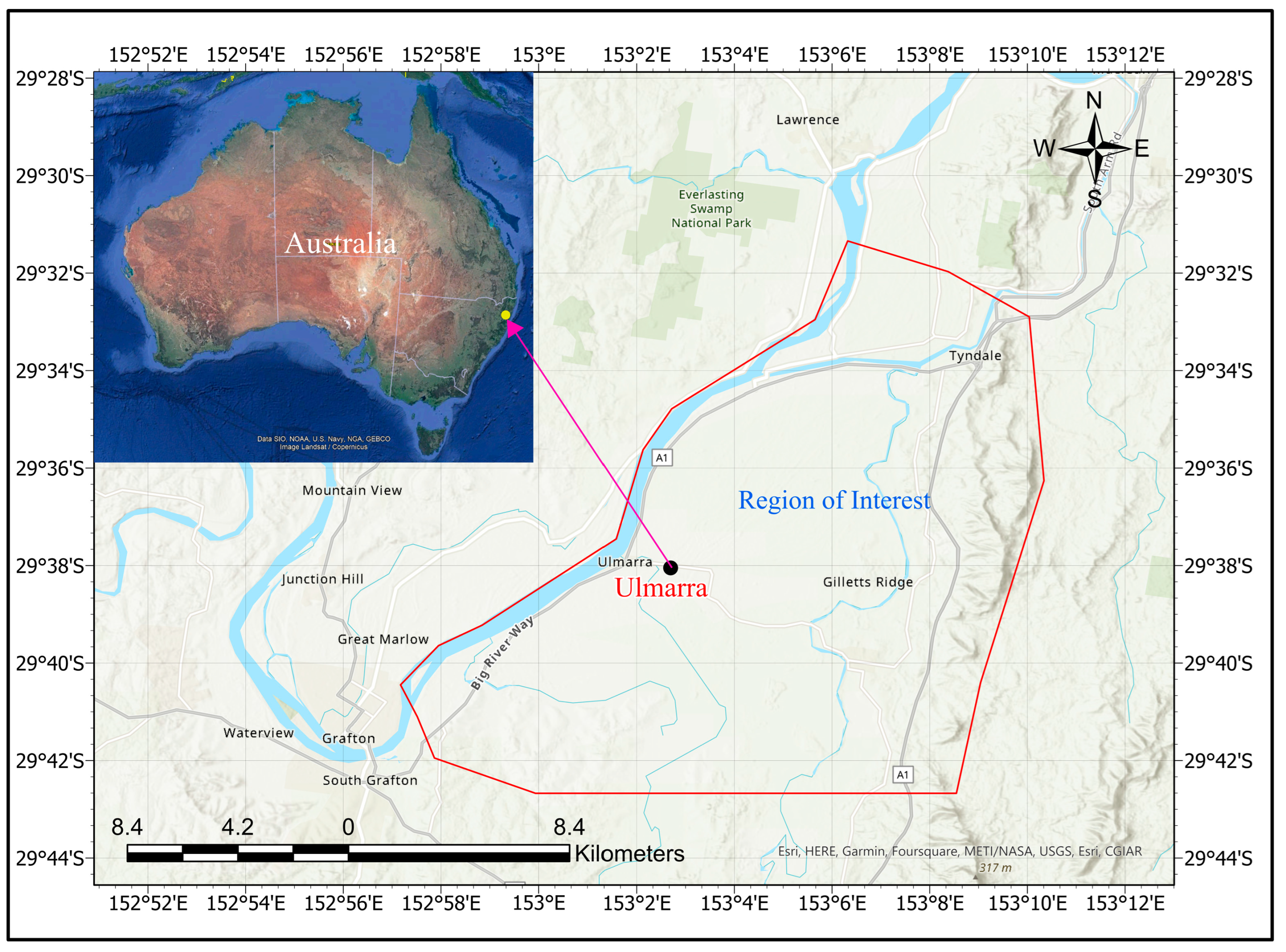
2.1. Study Area

Deep learning techniques, as demonstrated in many image classification studies, have great potential for improving flood mapping accuracy. Therefore, to compare the classification accuracy of our selected CNN-based deep learning models, Ulmarra was selected as the study area. Ulmarra is located on the North of New South Wales, Australia, and geographically located on latitude 29°37′50″ S and longitude 153°1′40″ E, flanked by the regional centre of Grafton on the southwest (Figure 1). A small town bounded by Clarence River, it had a population of 779 people according to the 2016 Census and had experienced widespread floods before the 28 February–3 March 2022 events. On 28 February 2022, due to a large amount of precipitation, the Clarence River rose significantly in under two hours, breaching the levee designed to protect the community. By midday of 1 March 2022, the town recorded an unprecedented flood. Ulmarra suffered minimal property damage and disruptions due to power outages during the flood event.

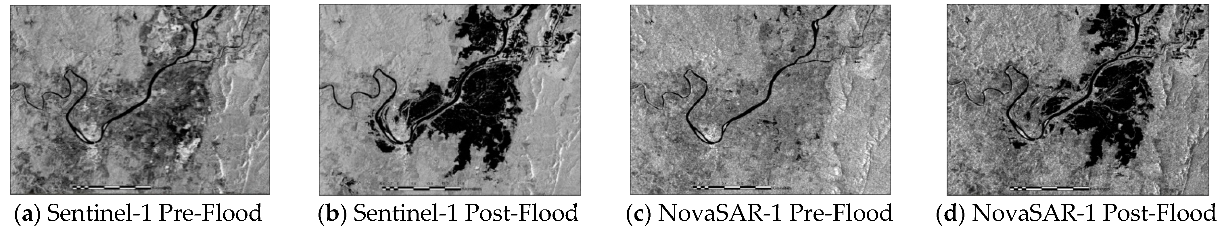
2.2. Dataset

Four SAR datasets from two different sensors were acquired over the study area. The first pair of datasets collected includes NovaSAR-1 pre-flood and post-flood images for 17 April 2021 and 5 March 2022. NovaSAR-1 is one of the low-cost S-band SAR missions launched in 2018 (

Table 1. Experimental SAR images used in this study.

Sensor	NovaSAR-1	NovaSAR-1	Sentinel-1	Sentinel-1
Band Used	S-dual polarised (HHHV)	S-dual polarised (HHHV)	C-dual polarised (VVVH)	C-dual polarised (VVVH)
Spatial Resolution (m)	50	50	5 × 20	5 × 20
Date	17 April 2021	5 March 2022	18 February 2022	3 March 2022
Product Type	SCD	SCD	GRD	GRD
Remark	Pre-flood for training	Post-flood for testing	Pre-flood for training	Post-flood tor testing

). The small SAR satellite is designed to provide medium spatial resolution (6–50 m) imagery for Earth observation, including flood monitoring, and is, to some extent, expected to overcome the limitations of low- and high-frequency SAR missions [48]. While data from the sensor has been applied in different natural resource management fields, not much has been exploited for mapping natural disasters, especially floods. Interestingly, as the use of SAR-derived measurements continues to grow and contribute immensely to hazard mapping such as floods, the data from this sensor is now of great interest to researchers. In this work, dual-polarised ScanSAR_195 km_HHHV (SCD Wide) swath (50 m ground resolution) datasets were acquired from CSIRO NovaSAR-1 National Facility Datahub as presented in Table 1. The ScanSAR wide mode is usually emitted in a variety of polarisations and reduced resolutions (30 m–50 m) and is suitable for large-area monitoring. For this study, dualCo-Cross polarized datasets were used (Table 1 and Appendix A:

Table A1. Location, sensing date and image name can be downloaded from the CSIRO NovaSAR-1 National Facility Datahub [69].

Location	Sensing Date	Image Name
Ulmarra	17 April 2021	NovaSAR_01_21984_scd_29_210417_005131_HH_HV
Ulmarra	5 March 2022	NovaSAR_01_32067_scd_220305_121059_HH_HV

)

Secondly, Sentinel-1 C-band pre-flood and post-flood images for 18 February 2022 and 2 March 2022, consisting of dual-polarised VV+VH Interferometric Wide (IW) swath mode, Ground Range Detected (GRD) (20 m ground resolution) datasets were downloaded from the European Space Agency Copernicus Open Access Hub (Table 1, Figure 2 and Appendix A:

Table A2. Location, sensing date and image name can be downloaded from Copernicus Open Access Hub [70].

Location	Sensing Date	Image Name
Ulmarra	18 February 2022	S1A_IW_GRDH_1SDV_20220218T190635_20220218T190700_041971_04FF93_F972
Ulmarra	2 March 2022	S1A_IW_GRDH_1SDV_20220302T190635_20220302T190700_042146_050598_23F0

).

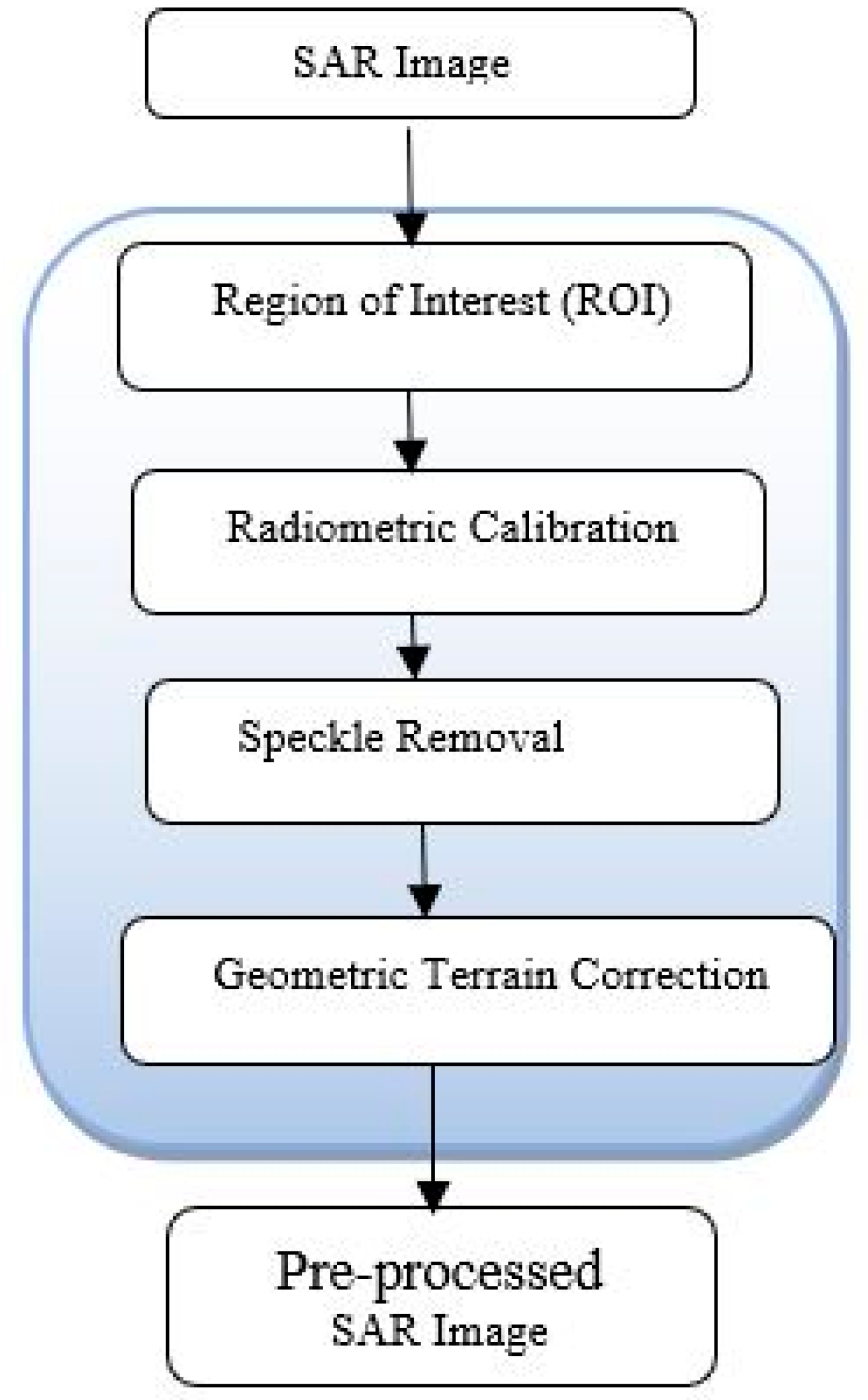
2.3. Image Pre-Processing

Given the inherent speckle noise and geometric errors often associated with SAR data, the need to improve data quality to achieve robust performance metrics cannot be overemphasized. SNAP 8.0 (Sentinel Application Platform) was used to perform the pre-processing tasks (Figure 3). Both Sentinel-1 and NovaSAR-1 were collected in UTM Zone 56J/WGS84 coordinate systems, which consequently facilitated the creation of the intersections for all images. We clipped all data to the study area by creating subsets using the SNAP toolbox. We also applied radiometric calibration to calculate the sigma nought values; however, this step did not apply to NovaSAR-1 as datasets emitted by the SSTL-Image Formation Processor-IFP are fully radiometrically calibrated images. Speckle reduction was performed using multi-looking processing parameters to minimise the effect of noise. Furthermore, geometric Doppler terrain correction was performed by applying SRTM 3s DEM to easily oversee geometric errors due to the side-looking geometry of the SAR systems. The co-registered sigma nought datasets of Sentinel-1 VV and NovaSAR-1 HV polarisations were exported as one band Geotiff image file for CNN-based deep learning techniques as shown in Figure 2.

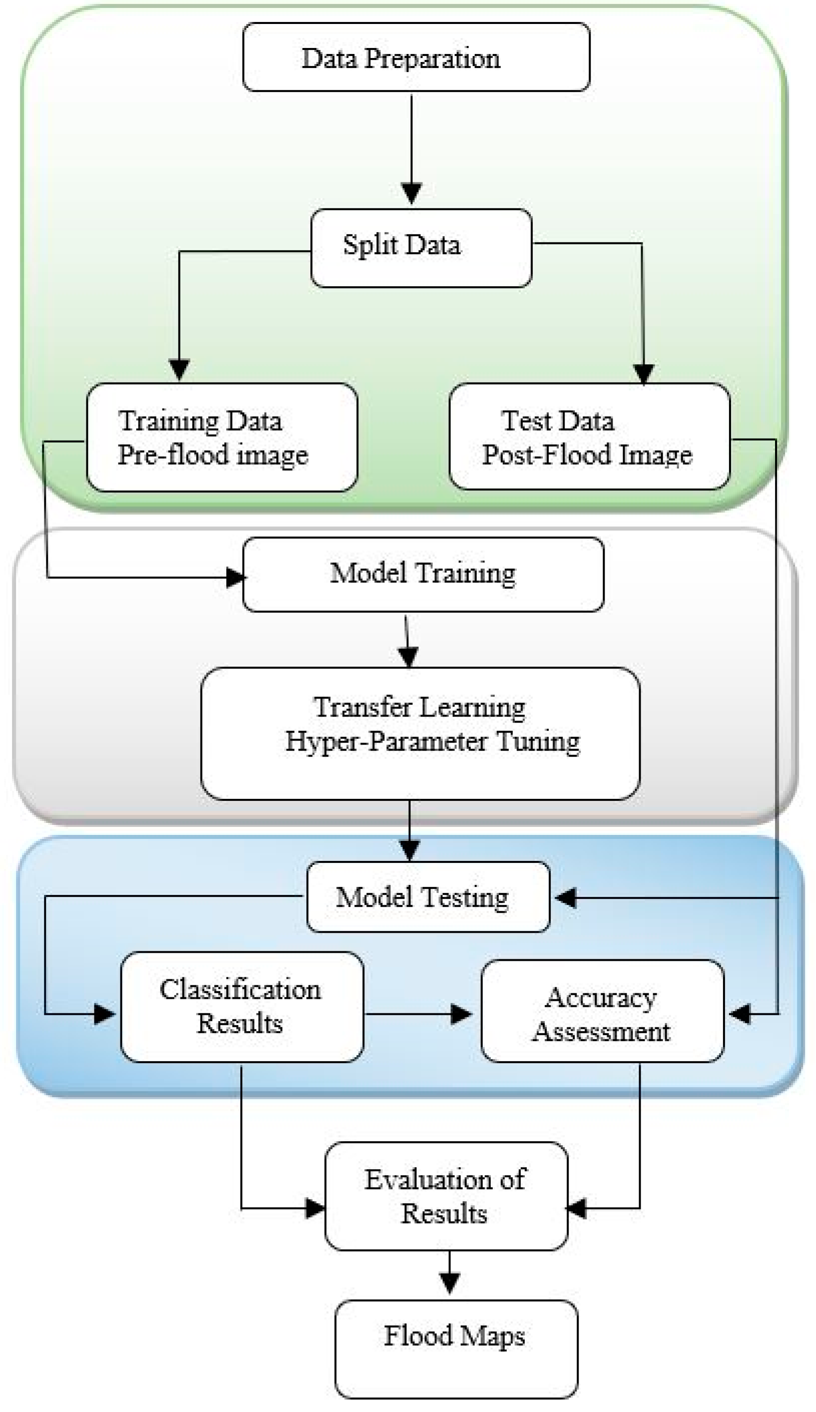
2.4. Data Preparation and Labelling

A challenge often associated with the SAR dataset is the non-availability of large-scale labelled training data compared to optical datasets. In this supervised CNN-based deep learning technique, the unlabelled pre-processed Sentinel-1 sigma0_VV_db (18 February 2022) and NovaSAR-1 sigma0_HV_db (17 April 2021) pre-flood datasets were imported to ArcGIS Pro 3.0, with all data georeferenced and projected to the same UTM Zone 56J/WGS84 coordinate systems. To improve our classification results and determine the actual flooded areas, we prepared the pre-flood images (as reference data) for training purposes. The images were converted to 8-bit unsigned RGB 3-band composite images suitable for deep learning. Since SAR data is generally complex and less intuitive [28], and the performance of a CNN model largely depends on the quality and amount of training sample datasets, we relied on pre-processed pre-flood datasets from Sentinel-1 and NovaSAR-1 imagery, as well as an ESRI World dataset, to manually create a large amount of image annotations required to train convolution neural network models for highly accurate feature extraction and pattern recognition [30]. The training data is characterised by different landcover types such as river, built-up area, forest vegetation, crop/cultivated land and roads. For this study, a detailed specification of pre-flood and post-flood amplitude datasets is provided in Table 1. The decision to use pre-flood data for training is three-fold. Firstly, it was used to distinctively clarify the extent of the flood as permanent water also existed in the area prior to the flood disaster. Secondly, the training data were used to test the generalisability of the trained CNN classifiers (i.e., to evaluate the performance of the trained model on completely unseen post-flood data) as this is a way of evaluating model performance [23,30]. Thirdly, it was used to address any uncertainty relating to post-flood water characteristics with different datasets. In this study, we separately trained two pre-flood datasets from NovaSAR-1 and Sentinel-1 imagery with different wavelengths, polarisations, incidence angles, spatial resolutions, product types, sensor modes and imaging dates. Overall, a similar outcome was achieved.

In generating training data, this study experimented on two types of classifications, namely, binary and multiple categories. While the Sentinel-1 dataset was trained for both binary and multiple classifications, the NovaSAR-1 dataset was trained using the binary classification due to its low resolution. To perform this, the Training Sample Manager pane of ArcGIS Pro was used to create the class categories from our classification schema. This step furnished us with vital information as to the size and number of samples and often plays a significant role in improving the accuracy of a classification model. To collect training samples from the input data sets, polygons were created around the pixels in the schema with corresponding class values.

2.4.1. Data Augmentation and Generation of Training Datasets

Prior to feeding the training CNN models, we converted the annotated Sentinel-1 and NovaSAR-1 vectors into a suitable deep-learning training dataset. However, due to the insufficient memory footprint on the computer hardware to process a whole image in its original resolution in deep learning, the class training samples are generated and trained on small sub-images called image chips [49,50]. This step was performed to address the memory limitations rather than improve the accuracy of the model [50]. The generation of training sets in this study included resampling the input image at a specified tile size of 256 × 256 pixels. The stride parameter was set to 128 × 128 pixels to ensure an overlap of 50% across the pixel tiles, which helped to overcome border artifacts commonly associated with CNN-based image segmentation [4].

We experimented on different rotation angles and observed that image chips increased as the value tends to 1 degree, with 0 degree being no rotation and no additional chips. Considering the balancing of the feature class, we decided to use a rotation angle of 30 degrees to generate additional image chips, which improved our model accuracy. To eliminate the unwanted image chips for training purposes, especially those that did not capture training samples, the software was tasked to output only feature tiles. Furthermore, the appropriate training metadata format (i.e., classified tiles) was specified to create label and image chips from the polygon shapefile for pixel-based semantic segmentation. These pairs of chips (often called tiles) have corresponding locations, and they consist of sub-images containing the feature of interest and indicate the RGB values of the input feature. The label chip is a raster with information about the class number of the pixels derived from the training polygon [49]. Other outputs of this step consist of feature class statistics, metadata files (i.e., ESRI model definition and accumulated-statistics) and a map file containing a list of corresponding images and labelled chips. More importantly, the output herein supports the implementation of third-party deep learning frameworks such as Keras, Google TensorFlow and PyTorch.

2.5. CNN Implementation and System Specification

Deep learning was implemented using the ArcGIS Pro Geoprocessing tool with the Image Analyst extension. The simplified workflow does not require the use of specific computer programming skills. Given the large amount of training sample data in this experiment, each of the multiple layers in the convolutional neural networks was required to extract features in the image. Therefore, we relied on a 40 GB RAM, NVIDIA GeForce RTX 3060 with 8 GB of dedicated GPU memory to perform our model training and inferencing.

2.6. CNN Deep Learning Models

The motivation to use CNN in this experiment stems from its widespread application in computer vision and image classification analysis. The use of convolutional neural networks (CNNs) has brought about a large and important improvement in pattern recognition. During detection, each neuron is localised within the region of interest of the input image, thus allowing it to greatly reduce training time and easily overcome overfitting, especially for a large dataset. The CNNs, unlike traditional neural networks (NNs), have significantly fewer trainable parameters, making the network computationally efficient. The CNNs models have been used to extract object and pixel-based features [51]. Therefore, in the next section, we examined the three CNN-based models used in this study.

2.6.1. U-Net Model

The U-Net model is an encoder–decoder model originally designed for biomedical image segmentation [52]. It has been widely used for research due to its robust prominence and well-defined structure [27]. In recent years, the occurrence of tiny and fine-grained targets in remote sensing data has led to the application of the model for better spatial refinement. For this reason, it is now the most widely used encoder–decoder design and has now been used in many research studies including remote sensing applications [27,53].

In this study, the encoder part of the neural network (i.e., ResNet), is a pre-trained convolutional backbone capable of high-level feature extraction, while the decoder helps to precisely localise features in the image tile [4,27,49,52,53]. The model was separately trained on NovaSAR-1 and Sentinel-1 labelled SAR pre-flood datasets and tested on the post-flood image to detect flood and determine the accuracy of model generalisability. We re-implemented U-Net in this study due to its demonstrated ability to achieve robust performance in pixel-based semantic segmentation, especially in the mapping of SAR-based floods, as previous studies have shown.

2.6.2. PSPNet Model (Pyramid Scene Parsing Network)

The PSPNet model is a widely known image segmentation model and can be trained to extract pixels in a raster image. This model was invented as an improvement over the fully convolutional network (FCN) segmentation model. It became handy in capturing the global context of a whole image as opposed to FCN pixel-based classifiers. It uses a pyramid parsing module to develop the global context of an image for predictions via local-based context aggregation, hence demonstrating better and more robust performance [54].

Like the U-Net model used in this study, PSPNet was trained on labelled SAR-pre-flood datasets with ResNet as the encoder (i.e., a pre-trained CNN backbone) to extract high-features in the input image, while the decoder played an important role in taking features in the encoder to predict results. For better performance, this study applied PSPNet with the U-Net-like decoder known as the feature pyramid network (FPN), which has learnable parameters capable of capturing small details and generating a high-resolution output. The whole post-flood images were used to test the generalisability of the model. Our decision to use PSPNet in this study stems from its ability to achieve compelling results in image classification as noted in [49,54]. The PSPNet model, according to [54], won the ImageNet Scene Parsing Challenge 2016 and has been highly cited and applied in many computer vision and Earth observation studies since then.

2.6.3. DeepLabV3 Model

DeepLabV3 is an encoder–decoder semantic segmentation model developed as an improvement over DeepLabV2 [49,55]. DeepLapV3 uses atrous convolution and has also experienced significant improvement in its Atrous Spatial Pyramid Pooling (ASPP) module compared to the CRF (Conditional Random Field) used in its previous versions [56]. The modifications in DeepLabV3 improved high-level features extraction in global context with increasingly better performance [57]. For this reason, in this study, DeepLabV3 was used to separately train our datasets with ResNet, particularly the ResNet 152 convolution back backbone, for the classification of each pixel to their corresponding classes. The use of DeepLabV3 in this study is due to its ability to achieve comparable performance metrics with other classifiers such as U-Net and PSPNet on the PASCAL VOC 2012 semantic image segmentation benchmark [55].

2.7. Convolutional Backbones

Convolutional backbones are feature extractors in the input layer of a CNN architecture, and they perform the specific function of extracting features for object and pixel image segmentation [27]. The two commonly used backbones are the ResNet family and the Vintage architecture, while others include DensNet, DarkNet and ImageNet. The ResNet backbones have shown superior performance in terms of accuracy in Earth observation image classifications over other convolutional architectures [27,58].

Several studies have shown that the depths of convolutional backbones that have been used in remote sensing are not the same as the depths of best performing models used on datasets in computer vision [27]. It is known in the field of computer vision that a deeper backbone, such as ResNet 152, has better performance than shallower variants such as ResNet, 101, 50, 34 and 18 [27,59]. The deeper a CNN model, the better because it contains more hidden convolutional layers capable of accurately classifying 1000 classes and can easily overcome the tiny objects and fine-grained targets that characterize remote sensing data [27].

In this work, we experimented on the ResNet family, especially the recent variant ResNet 152. The 152 layer-deep residual network is a preconfigured model trained on the ImageNet dataset containing over 1 million images., The authors of [27] argued that the deeper a model, the more parameters it has. However, due to many insufficiently trained parameters arising from small datasets in Earth observation imagery, they are not frequently used [27,60] but can easily oversee spatially tiny targets in Earth observation compared to shallower models. As observed in our experiment, ResNet 152 model can overfit on a small dataset due to its depth, which we addressed by performing data augmentation to increase our training samples.

2.7.1. CNN Model Training

In this study, we trained the CNN models using the geoprocessing tools of ArcGIS Pro 3.0 Image Analyst extension. The model training was implemented using the image chips generated in Section 2.4.1 Each proposed CNN model in this work was trained separately, and model training parameters were populated accordingly. The different training epochs, (i.e., the number of times the dataset passes forward and backward through the convolutional neural network) were tested and set to 50 for best results in the whole experiment. The software was tasked to grid search the optimum learning rate from the learning curve during each training stage.

We performed hyperparameter optimisation using varying batch sizes. As mentioned before, the ResNet family, especially ResNest 152, was chosen as the convolutional backbone architecture for this experiment due to its depth and relatively low application in Earth observation. During the training process, early stopping was implemented as too much training can lead to overfitting on the training model. The early stopping technique ends the model training when model accuracy no longer improves regardless of the maximum epoch specified. To validate the models, some input training samples were used as shown in

Table 2. Training sample summary.

Category/Dataset	Sentinel-1	NovaSAR-1
Binary Class	Water Non-Water	Water Non-Water
Image tiles for Training and Validation	2120	2196
Image tiles for Validation
Multi-Class	Water Built-up Forest Cropland/Cultivated	Not Applicable
Image tiles for Training and Validation	1980

. [4,61]. While training was in progress, training and validation losses for each iteration were monitored to ascertain the performance of the neural networks.

Afterwards, an ESRI model definition file (EMD), (i.e., a configuration file that contains parameters to run deep learning model inference) and a deep learning package (.dkp), which also contains an ESRI Model Definition file, as well as a trained model metrics file, are generated. Another output includes a loss graph showing training and validation losses, which helps to visualise and diagnose the performance of the model as well as to identify where tuning is needed. In this work pipeline, the trained model file extension is dependent on a deep learning framework. Specifically, ArcGIS Pro implemented the PyTorch backbend for our classification. For clarity, we present a CNN-based deep learning workflow for our study in Figure 4.

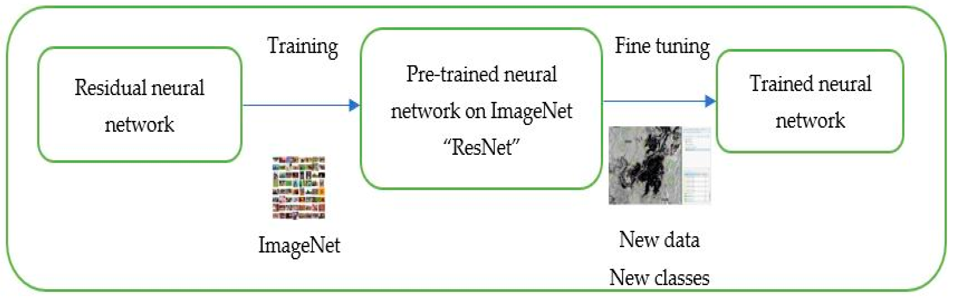
2.7.2. Transfer Learning

Building a neural network can be challenging given the vast computing and time resources required, as well as the complexities associated with the input datasets on which these models are trained. To reduce training requirements, neural network parameters can be reused from the previously learnt features to fine-tune a new model; this is known as transfer learning. This method is an optimiser, which can speed up training time and improve model performance and generalizability [4,62].

In machine learning, transfer learning refers to the process of using a pretrained model as the starting point for a second task with a similar convolutional neural backbone. The extraction of information in CNNs is generally implemented using a hierarchical method. While the first convolutional layer detects the edges and corners of an image, the last layer gives more sophisticated information about extracted features. These CNNs structure make them well suited for transfer learning [4].

To perform image classification task in this study, we implemented the pre-trained model approach of transfer learning in Section 2.7.1, which allowed us to specify a pre-configured neural network as the convolutional architecture for training the CNN models, as shown in Figure 5. ResNet, a convolutional backbone, which was pre-trained on the ImageNet database, acts as the encoding part of the neural networks for the extraction of complex features such as edge detection and pattern recognition. The fine-tuning was performed on our new labelled datasets (SAR data) to evaluate the training performance of U-Net, PSPNet and DeepLapV3 models. [4].

2.7.3. Neural Network Hyper-Parameter Tuning

Hyper-parameters are the configurable variables that govern the model training process, and they are usually fixed during training. In this study, we ran multiple model training trials for U-Net, PSPNet and DeepLabV3 by varying their training parameters to obtain the best performance in Section 2.7.1. After some multiple training trials, we set the epoch to 50, varied the batch size and grid-searched the optimum learning rates for the whole training. This was implemented manually and found to be computationally expensive. For this reason, we implemented a trade-off between parameters that have been tested but were found to have no significant impact on the model performance and those parameters that have a significant impact on the model performance. For computational efficiency, we opted for the latter.

2.8. Accuracy Assessment and Confusion Matrix

To further test the performance of the models and their ability to generalise varying complex and dynamic environmental settings, especially for operational flood conditions, we performed both binary and multi-classification accuracy assessments using unseen post-flood datasets (i.e., Sentinel-1 and NovaSAR-1). A stratified random approach of at least 500 randomly distributed points was used. These points were distributed such that they were proportional to the relative area of each class. This was followed by the generation of a confusion matrix to determine the overall kappa index of agreement. This approach describes how well a model has performed much better than just training accuracy as, sometimes, the training accuracy metrics can be misleading.

Neural Network Evaluation Metrics

The evaluation of model performance is an essential part of the CNN-based deep learning workflow. In flood water detection, confusion matrix has been frequently used for measuring model performance as this helps to assess how well different classification models have performed. For this purpose, four quantitative evaluation metrics have been chosen to evaluate the accuracy of water extraction as well as other classes. The assessment criteria were overall accuracy (OA), recall (R), precision (P), recall and F1-score.

Overall accuracy is the percentage of training samples that are correctly classified. Accuracy for binary classification can be mathematically expressed as follows [30,63]:

$$\mathrm{OA}=\frac{TP+TN}{TP+FP+TN+FN}$$

(1)

Recall (R) is expressed as the ratio of number of positive samples correctly classified as positive to the total number of positive samples and mathematically represented as follows [30,63,64]:

$$R=\frac{TP}{TP+FN}$$

(2)

In multi-classification, it is hard to generalize performance; thus, we examined the results based on class. For this reason, we use recall values of each class for both binary and multi-classification.

Precision is the ratio of numbers of positive samples that are correctly predicted to the total number of samples classified as positive and can be expressed as follows [30,63,64]:

$$P=\frac{TP}{TP+FP}$$

(3)

F1-Score is defined as the harmonic mean of recall and precision and can be expressed as follows [30,63,64]:

$$F=\frac{2\ast Recall\ast Precision}{2\ast Recall\ast Precision}$$

(4)

Our datasets are unbalanced and, therefore, have unequally distributed classes. For this reason, the F1-Score was used to measure the results between the different classes.

In the above equations, TP is True Positive, FP is False Positive, TN is True Negative and FN is False Negative.

3. Results

3.1. Training Data Comparison for Binary Classification

In this section, we present our binary classification results for training datasets using four model metrics. The quantitative comparisons in Figure 6a–c represent the overall performance of the three CNN deep learning models selected for this study.

Figure 6a,b represent the model training results for the Sentinel-1 and NovaSAR-1 pre-flood datasets, respectively. The main differences between the two sets of SAR data are the polarisations, ground resolutions and sensing periods. As can be seen, the models do not show any significant difference in performance. After training each model separately, U-Net + ResNet 152 achieved a marginally higher average overall accuracy and showed strong recall/precision statistics in the extraction of permanent water pixels. In addition, the three models achieved strong recall, precision and F1-score statistics, which implies that there were a few missing water pixels in our prediction, thus decreasing the amount of manual cleaning that was performed. Overall, Figure 6c summarises the overall accuracy of the two training datasets. As can be seen, NovaSAR-1 compares well with Sentinel-1 in overall accuracy, except for the 1% loss during PSPNet model training.

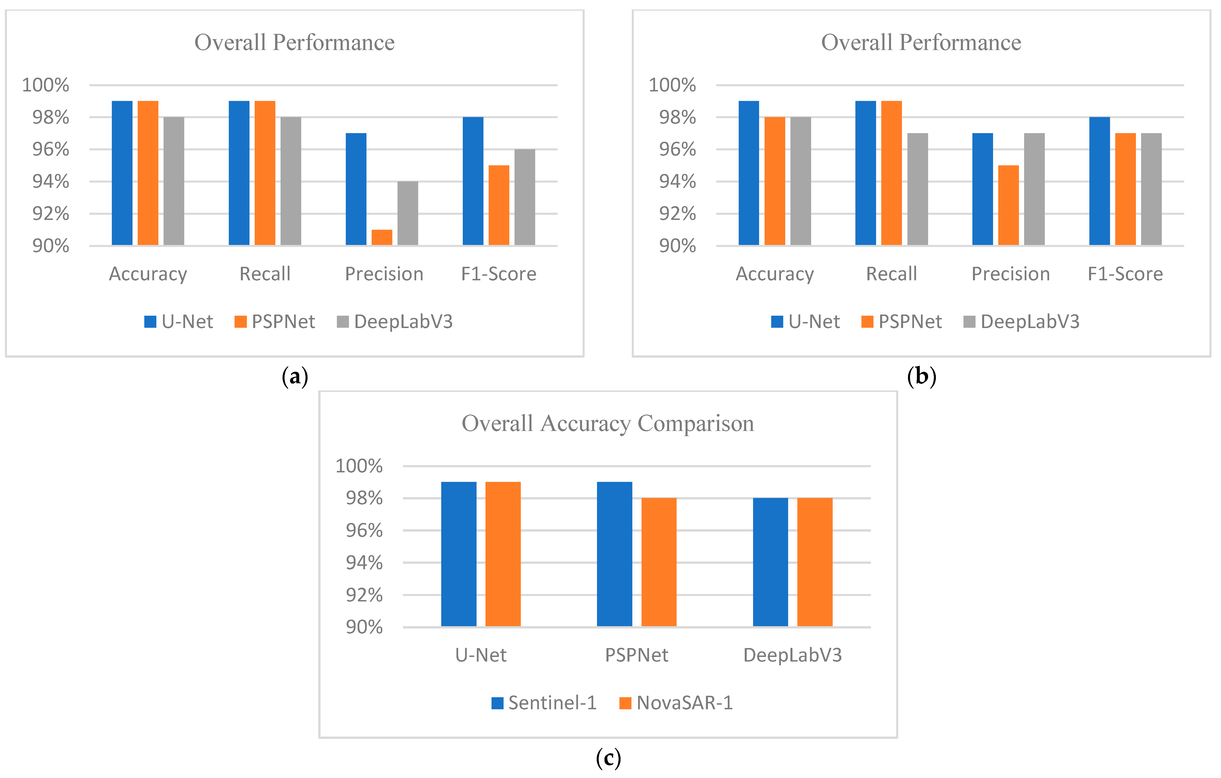
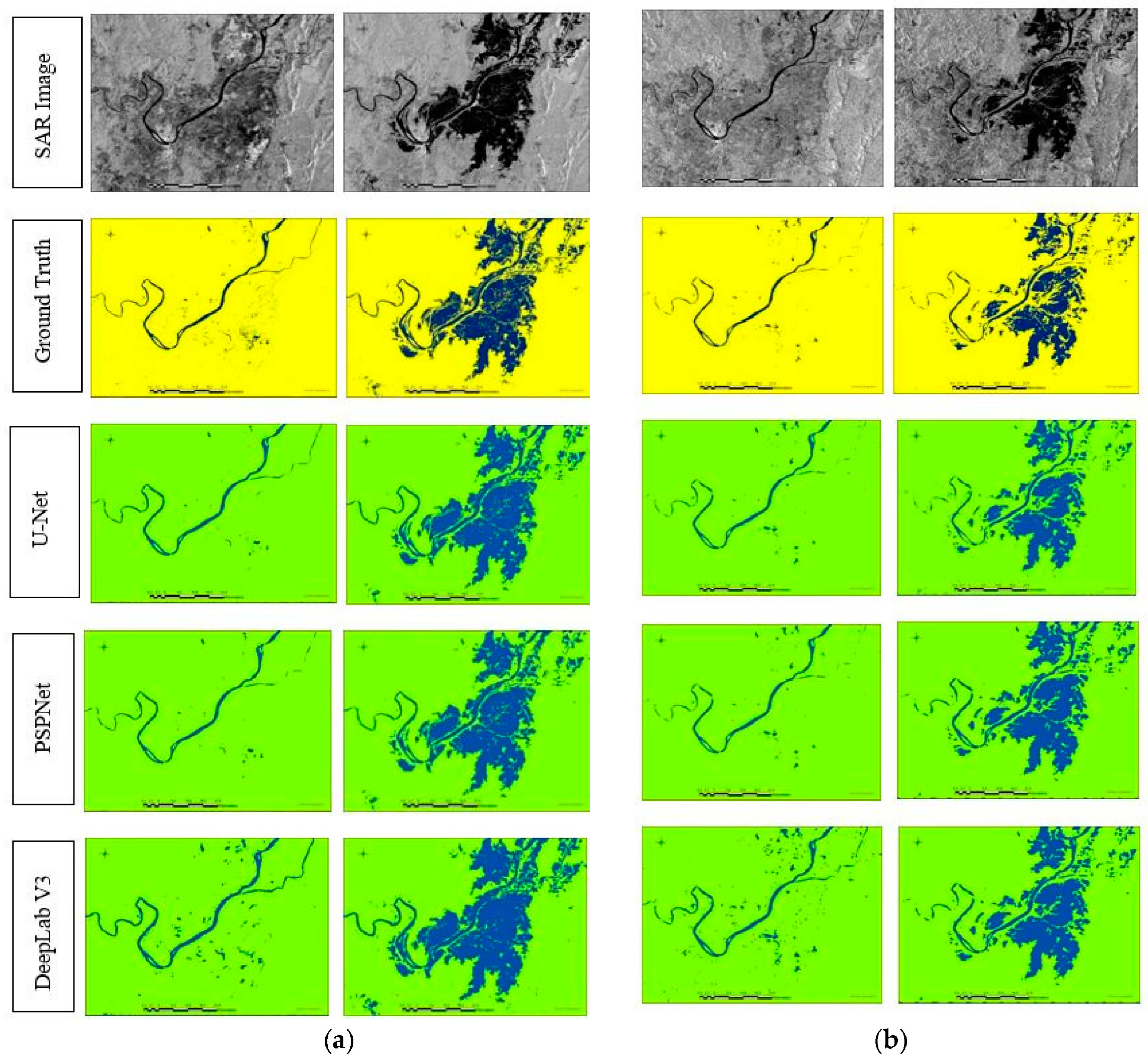
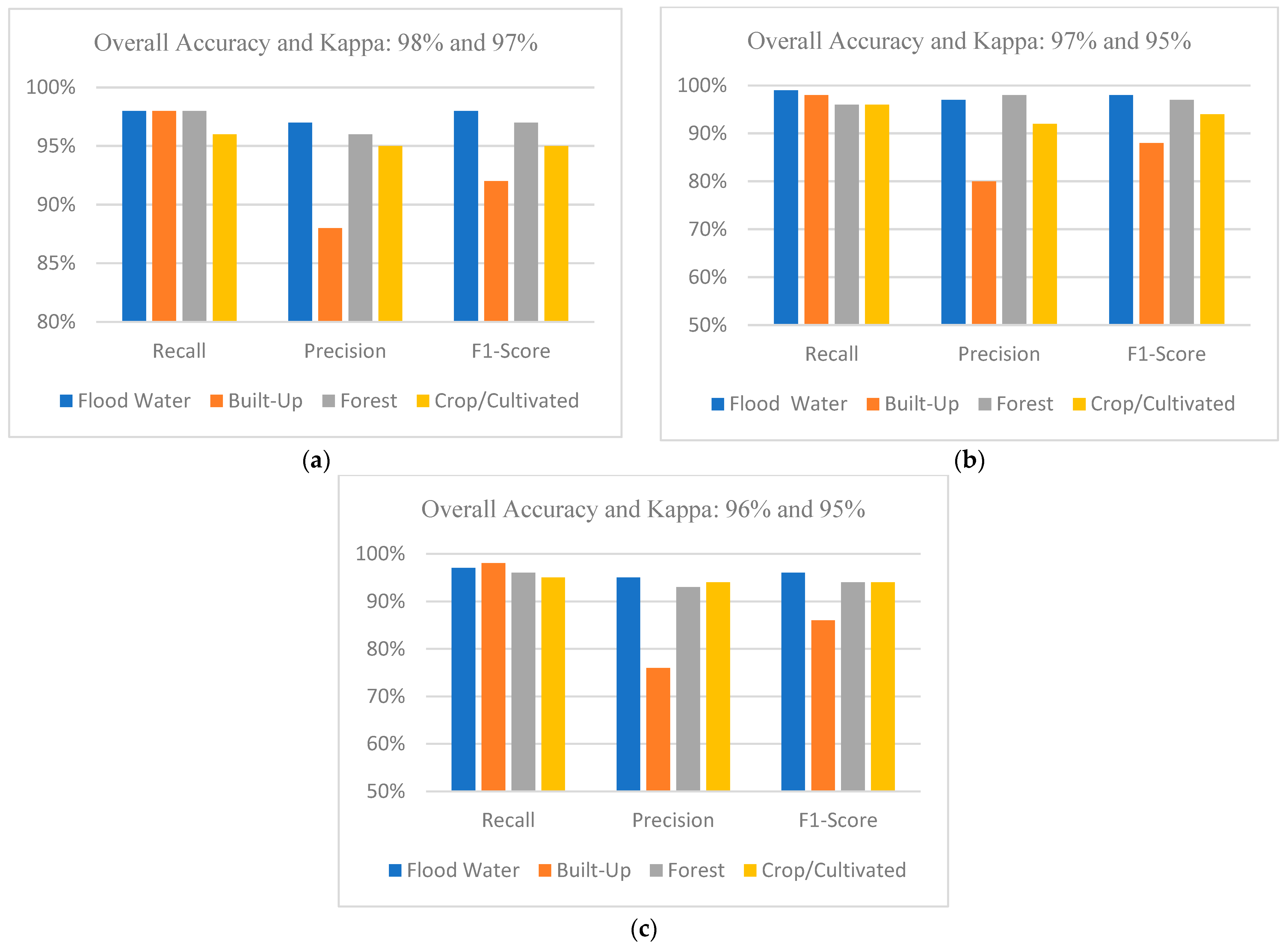
3.2. Test Data Analysis for Binary Classification

We present the test results of both seen and unseen binary classifications for both Sentinel-1 and NovaSAR-1 in Figure 7a,b:

In this section, we present the analysis of the inference performed on the unseen (i.e., post-flood) datasets from the trained models. Each model was performed in a slightly different manner in terms of the extraction of flood pixels and accuracy; despite this, the semantic segmentation outputs generally showed a much higher level of detail. For instance, while PSPNet + ResNet 152 maintained flood and permanent water boundaries, with some insignificant false negatives, it showed a better ability to detect small and isolated water, as well as a strip of water, as can be seen in Figure 7a,b. DeepLabV3 + ResNet 152 did not perform well in maintaining flood and permanent water boundaries but showed how well it can extract small and isolated water. Generally, we noticed a few false positives along the flood and water permanent water boundaries. While U-Net + ResNet 152 appeared to have a marginally higher and more accurate feature extraction ability along the flood and permanent water boundaries, it also performed well in extracting small and isolated water as well as long and tiny strips of water. From our observation, the pixel extraction by U-Net showed minimal misclassification and substantially consistent details with the ground truth data, thus making the model superior to PSPNet and DeepLapV3.

Statistically, inference was performed on the trained models using the Sentinel-1 and NovaSAR-1 datasets, and, as can be seen, the models achieved good test results with a 99% average overall accuracy, as shown in Figure 8a,b below. Specifically, the 99% average overall accuracy obtained for U-Net + 152 in Figure 6c during the model training is consistent with that achieved during the testing stages. Overall, the results in Section 3.1 and Section 3.2. compare well and further demonstrate the generalisability of the models.

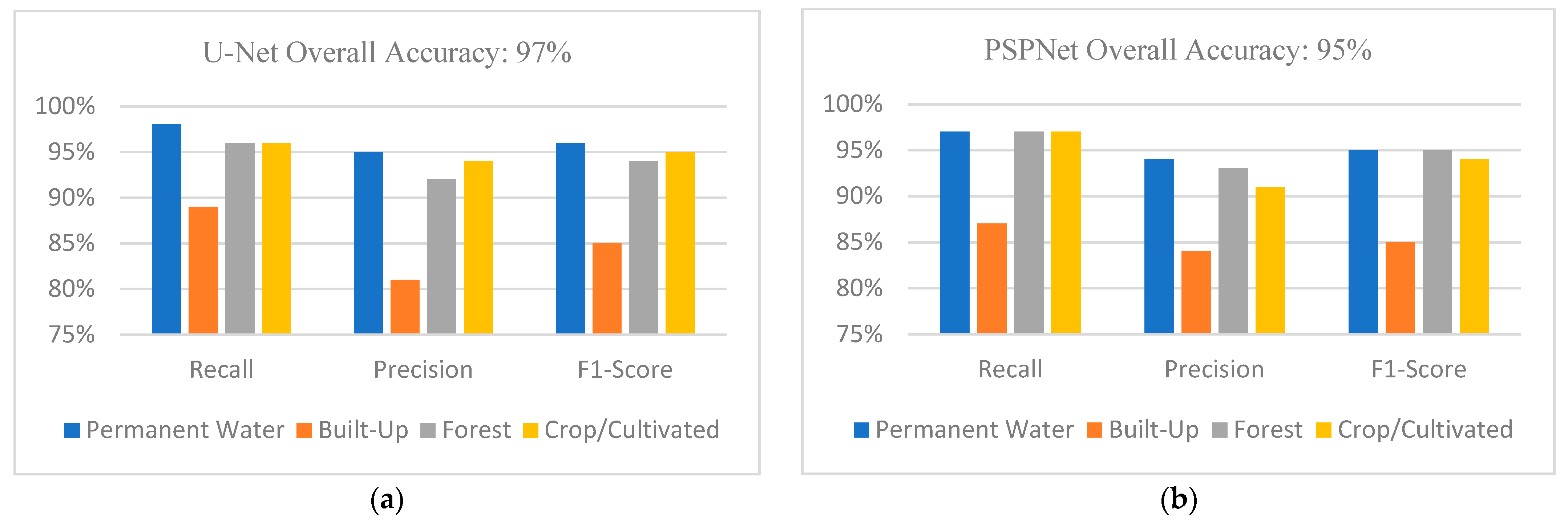
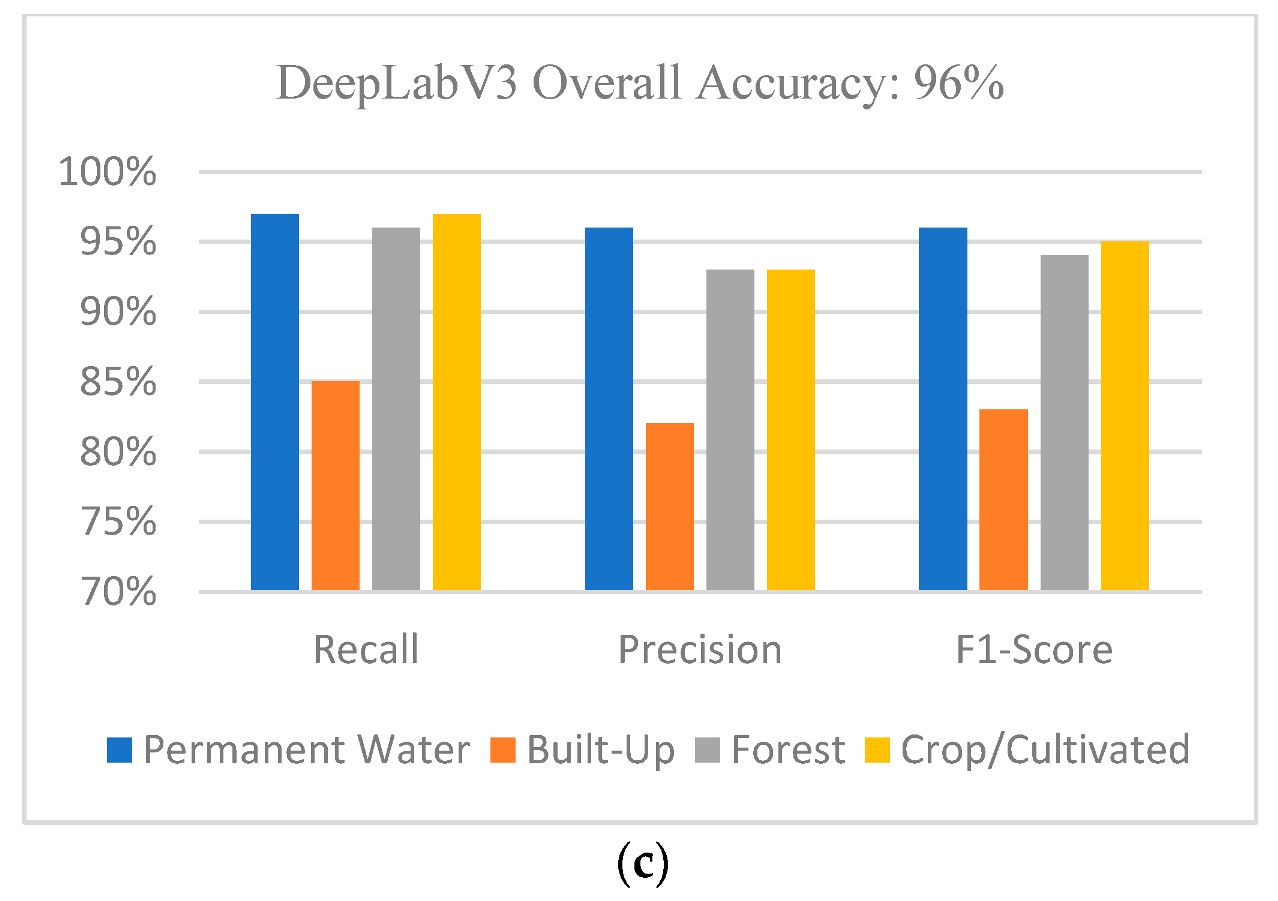
3.3. Training Data Comparison for Multi-Classification

The result from the training of neural networks for the multi-classifications showed that the three models performed well in each class. Given the high resolution of the Sentinel-1 dataset, we were able to classify the land cover into permanent water, built-up area, forest and crop/cultivated area. The idea is to establish a relationship among the classes and the extent to which each of these classes was affected during the flood disaster. To achieve this, we trained the three models using the pre-flood dataset and performed inference with the flood datasets to determine the flooded area, after which we carried out quantitative and qualitative analysis of the results.

The results of the network performance are shown in Figure 9a–c. As can be seen in Figure 9a, U-Net + ResNet 152 was trained with a 4 batch size, and a 0.0000014454 learning rate achieved the best accuracy. The overall accuracy reached 97%, i.e., 2% less than the Sentinel-1 binary classification accuracy. Interestingly, both achieved a similar recall value of 98% for permanent water. The built-up class showed some false positives, in which few forest pixels were classified as built-up areas. Similarly, the forest and crop/cultivated classes both recorded recall values of 96%. Overall, the three models performed well during training and produced a marginally different result across the evaluation metrics.

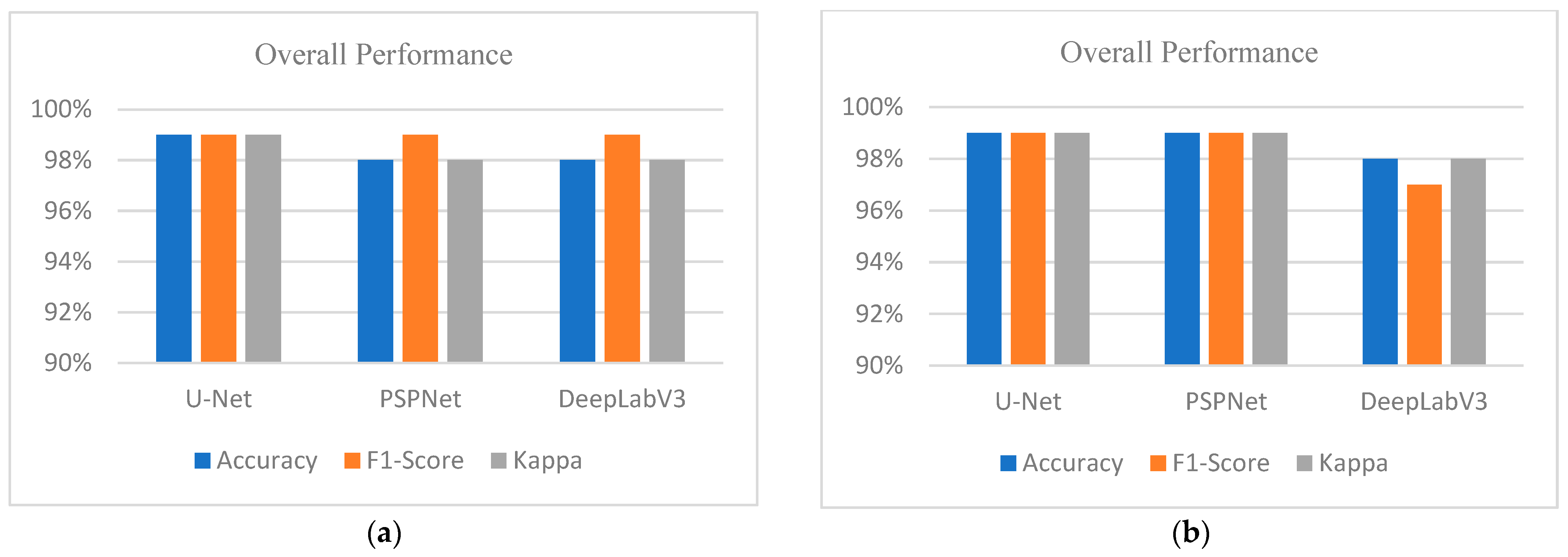
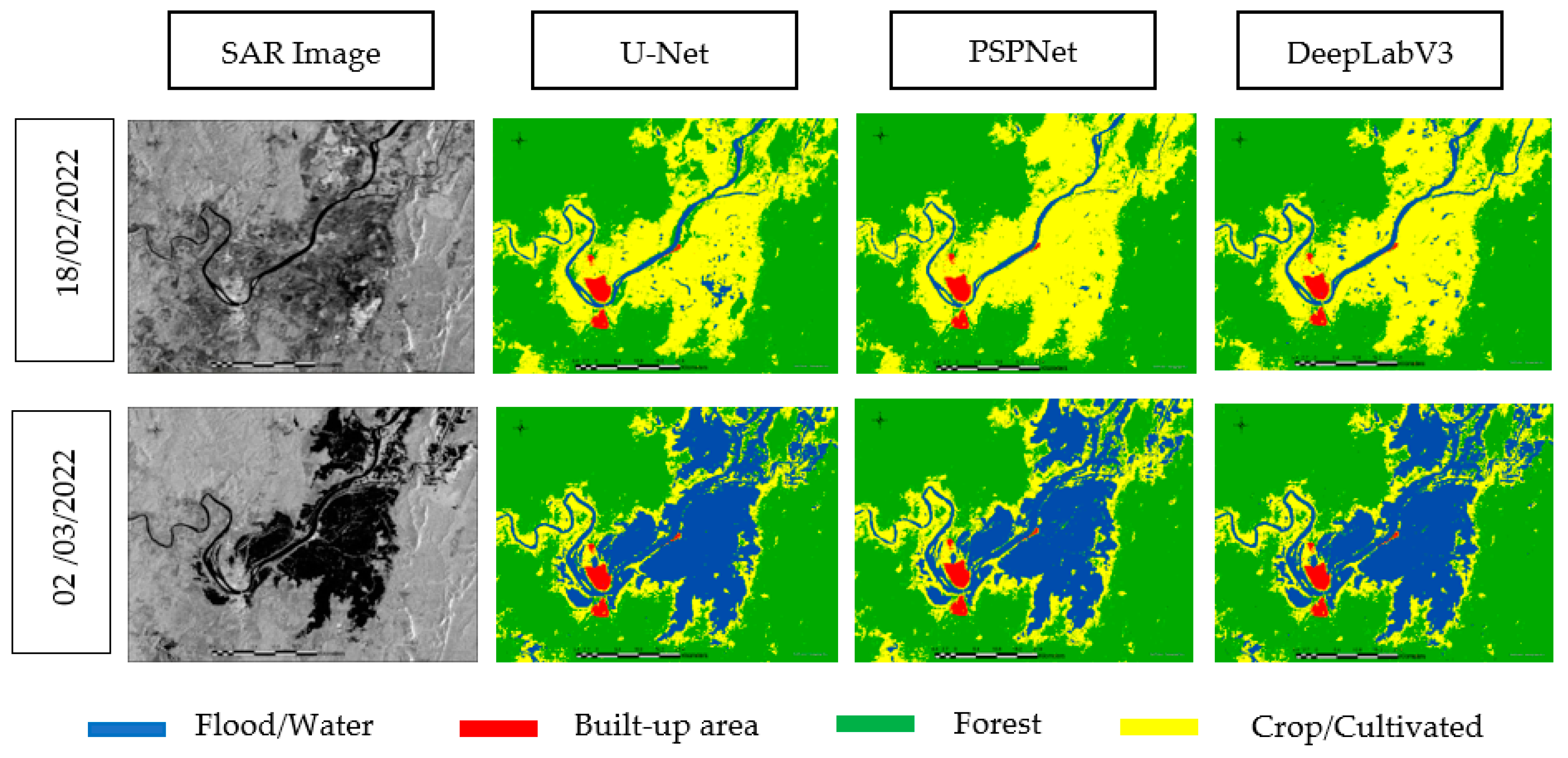
3.4. Test Data Analysis for Multi-Classification

The multi-classification results presented in Figure 10 enabled us to assess the impact of floods on other classes during testing. Our estimation from the ground truth showed that the flood event covered approximately 188.731 square kilometres and compared well with the U-Net + ResNet 152-based inference. In Figure 11a, the recall and precision scores for the flood class reached 98% and 97%, respectively, leading to an F1-Score of 98%, which indicates the presence of few false positives and negatives. It can be seen in Figure 10 that the U-Net model showed superiority in maintaining flood boundaries and improving the detection of large and small bodies. Similarly, PSPNet + ResNet 152 and DeepLabV3 + ResNet 152 produced F1-Scores of 98% and 96%, respectively, for this class.

The built-up area accounting for approximately 0.739 square kilometres achieved F1-score statistics of 92% for the U-Net model. On the other hand, PSPNet + ResNet 152 achieved an F1-score value of 88% and DeepLabV3 + ResNet 152 produced a value of 86%. In summary, U-Net gained 4% and 6% over PSPNet and DeepLabV3, thus outperforming the other models in classifying the built-up area. However, while the models were to delineate the built-up area, they could not identify few water pixels in some parts of the densely populated area. It is believed that the flood had receded in the affected areas when the image was captured.

Figure 10 shows a large extent of forest bordering the crop/cultivated area. In Figure 11a, the forest class achieved a recall value of 98%, with a record of some false positives, as 2% of the pixels were incorrectly classified when they should have been classified as crop/cultivated. In addition, it achieved a precision score of 96%, which implies that 4% of the pixels were omitted from the class and classified as built-up, leading to an F1-score of 97% for U-Net + ResNet 152. While the PSPNet + ResNet 152 achieved an F-Score of 97%, the DeepLabV3 + ResNet 152 scored 94%. Overall, the three models demarcated the forest extent as can be seen from the results, but the U-Net and PSPNet models produced the best classification performance for the forest class.

In this study, we estimated approximately 225 square kilometres of crop/cultivated area, of which approximately 188.732 square kilometres (corresponding to 84%) were flooded during the disaster. During our testing, the crop/cultivated area achieved a recall score of 96% and a precision value of 95%, suggesting the presence of some false negatives, as 5% of the pixels were incorrectly classified as forest and built-up areas. As a result, an F1-Score of 95% was obtained for U-Net + ResNet 152; the result is 1% higher than the F1-Score values obtained from the other models.

Overall, the models performed superbly and achieved similar outcomes, making them well suited for SAR-based flood mapping. The overall accuracy and Kappa achieved by U-Net + ResNet 152 are 98% and 97%, respectively. On the other hand, PSPNet + ResNet 152 achieved 97% and 95%, while the DeepLabV3 +ResNet 152 scored 96% and 95%, respectively.

3.5. Hyper-Parameter Tuning Results

In this section, we present the results of our hyper-parameter tuning experiment for the selected neural network models and backbone. We varied hyper-parameters such as batch size and epoch and grid-searched for the optimum learning rates, which are perhaps the most important hyper-parameter for each training.

As can be seen from the results in

Table 3. Hyper-parameter tuning results for binary classification.

Model + Backbone	Batch Size	Epochs	Learning Rate	Overall Accuracy
Unet+ Resnet 18	2	29/50	7.5858 × 10−6	99%
Unet+ Resnet 18	4	23/50	6.3096 × 10−6	99%
Unet+ Resnet 18	8	30/50	7.5858 × 10−6	99%
Unet+ Resnet 18	16	49/50	2.5119 × 10−6	96%
Unet+ Resnet 34	2	17/50	6.3096 × 10−6	99%
Unet+ Resnet 34	16	34/50	6.3096 × 10−6	96%
Unet+ Resnet 34	32	49/50	3.6308 × 10−6	97%
PSPN + Resnet 18	2	19/50	3.9811 × 10−3	99%
PSPN + Resnet 18	4	32/50	1.0965 × 10−3	99%
PSPN + Resnet 34	2	17/50	2.2909 × 10−3	99%
PSPN + Resnet 34	8	28/50	7.5858 × 10−4	99%
PSPN + Resnet 34	4	46/50	6.3096 × 10−4	99%
PSPN + Resnet 50	2	20/50	1.0000 × 10−2	99%

, varying the batch size, backbone and learning rates and setting the epochs can influence model performance. In this work, we noticed that with larger batch sizes, the training and validation losses decreased slowly, and it took more epochs to converge. Additionally, as we increased the depth of the neural network and batch size, the model became more difficult to train and sometimes became overfit. In contrast to larger batch sizes, smaller batch sizes proved to be effective in speeding up the processing time while still achieving high model accuracy, especially with deeper convolutional backbones. To reduce training time and improve computational efficiency, we lowered our batch sizes while increasing the depth of the neural network. In the process, the validation and training losses took less time to converge at fewer training epochs for many numbers of iterations. The training was automatically stopped during separate training times due to the implementation of the early stopping technique, after which we compared training and validation losses as well as overall accuracy, from which we selected the best-performing models.

3.6. Impact of Class Structure

In this study, the test results for our binary classification in comparison with multi-classification showed that the latter decreased in overall accuracy. For instance, in the multi-class category, U-Net, PSPNet and DeepLabV3 decreased by 1%, 2% and 3%, respectively. Overall, our binary classification achieved superior results.

4. Discussion

In this work, we demonstrated that CNN-based deep learning techniques performed very well on well-prepared SAR-based training samples. The achieved results suggest that these techniques are well suited for operational flood mapping given their ability to generalise different conditions over significantly large training datasets. The strong model performance obtained from our CNN-based model training and those achieved from the completely unseen post-flood image, which was never part of our training samples, further demonstrate it. We adopted this approach of testing the unseen dataset to overcome the findings in Kang et al. [23]. The authors argued that the test set captured in the training dataset is often small and has great randomness. Therefore, it cannot fully reflect model generalisability as it becomes difficult to measure model performance in other scenes [23]. As can be seen, the results from our unseen test set (i.e., whole post-flood image) in Figure 8a,b are comparable to the large training set used for permanent water detection (i.e., pre-flood image) in Figure 6a–c. Interestingly, the scores achieved helped to validate the generalisability of the models on different scenes. While we established that images with different polarisations can achieve similar model performance, we also noted that the detection capability of the models can improve with high-resolution imagery, especially for multi-classification.

Earlier in this paper, we introduced the work of Nemni et al. [4], Li et al. [18], Zhao et al. [30], Wu et al. [46], Katiyar et al. [47] and Kang et al. [23] using CNN-based deep learning for the extraction of flood pixels from SAR images over different locations and environmental conditions. Comparing the results presented in these studies to our study, we found that our scores are either similar or superior to the scores presented. Specifically, the result from Nemni et al. [4] showed that the U-Net + ResNet quantitative comparison used when considering Sagaing Region in Myanmar achieved an overall accuracy of 99%, which is comparable to our score, but recorded marginally lower recall/precision scores compared to our results. Similarly, Kang et al. [23] showed that the overall accuracy of FCN16 can reach 99%, which is comparable to our method. In another SAR-data-driven flood detection, Wu et al. [46] achieved an average IoU score of 86.33% and PA score of 95.75%. Furthermore, the overall accuracy score in [46] appeared to be similar to that of Zhao et al. [30], who achieved 95.95% for water and non-water classes, thus scoring about 3% lower than our best overall accuracy. However, ref. [47] compared to our method, they presented a marginally lower overall accuracy of close to 90%. Overall, the results presented in Section 3.2 and Section 3.4 are a proof of concept that our methodology can compete and even achieve superior scores for SAR-based flood mapping.

From our results, we observed that the U-Net model showed less complexity and a relatively low training time as well as a higher score, especially with the ResNet encoder. The ResNet backbone is known to have a better accuracy–parameter ratio, is less complex and can easily adapt to complex scenarios [65,66,67,68]. It can retain the original features of an image, thus making it well-suited for transfer learning [62].

A problem we noticed during the generation of input data was unbalanced classes. For instance, water had fewer class samples than other classes, leading to the models being biased towards classes with many samples and making the models learn more about the large samples than small samples. In this work, we tested four different shifts or rotations for the Sentinel-1 and NovaSAR-1 datasets to improve the distribution of the dataset among the classes. When 0-, 15-, 30- and 45-degree rotations were experimented during the resampling process, it was observed that the 30-degree shift significantly improved model performance over others as it generated a relatively balanced sample among the classes. Additionally, to deal with problems associated with class imbalance, we also applied the focal loss function during model training to obtain speedy convergence between the training loss and validation loss. The loss function focused on samples that would have been predicted wrongly by the models over those they can correctly predict, which was achieved via the down-weighting technique. The bias towards the majority class was significantly reduced and their total loss contribution was downsized.

Furthermore, the results from the loss charts in Figure 12 suggest how the CNN-based deep learning models we tested fit our training data (i.e., pre-flood Sentinel-1 and NovaSAR-1). Sometimes, models can be susceptible to poor performance on training data and hence produce large errors. In this case, we reduced the need for further training and downsized the potentially large training errors by augmenting our training samples. In this study, the validation loss and training loss metrics were used to evaluate the performance of the three models during training. These losses account for the errors produced by these models and determine the difference between the training and validation data. As can be seen from the loss charts below, however, the training and the validation losses are as low as possible, indicating some overfit. In training our sample data, an early stopping approach was implemented to prevent overfitting where a model became too complex for the training data.

5. Conclusions

In this work, we present the implementation of the near real-time deployment of a CNN-based transfer learning technique for a synthetic aperture radar (SAR)-derived flood data. The ArcGIS Pro deep learning workflow offered the possibility to implement U-Net, PSPNet and DeepLabV3 for automated, rapid and continuous flood mapping while achieving strong performance metrics over datasets with different polarizations, spatial resolutions and bands. The experimental results from our comparative study showed that U-Net marginally outperformed the other models, thus showing the good retention of image resolution during feature extraction and the generation of fine-grained class boundaries.

We not only demonstrated that CNN models trained on datasets from two different SAR sensors (i.e., NovaSAR-1 and Sentinel-1) [69,70], over the same area can achieve high performance scores but also sufficiently provided semantic segmentation outputs and statistics for both the seen tiles (pre-flood) and the completely unseen tiles (post-flood) to test the generalisability of these trained models. Overall, both trials produced similar results.

For real-time deployment, we found that the pre-trained model approach of transfer learning is a viable option for speeding-up model training and reducing training requirements as building a new neural network from scratch requires vast computing and time resources. Additionally, it was observed that the depth of a model can influence training time. For instance, while ResNet 152 demonstrated less complexity with remarkable model performance metrics, the shallower convolutional backbones were trained quicker.

Based on our hyper-parameter experimental results, we found that smaller batch sizes can be effective in speeding up the processing time while still achieveing high model performance metrics, especially when training a deeper convolutional backbone such as ResNet 152, with small computational resources.

Therefore, we conclude this paper with the following remarks:

• The adopted workflow can produce comparable or even superior results to some previous SAR and optical flood-based studies. The method not only speeds up inferencing but also does not depend on many ancillary data from other sources.
• One of the findings of this study suggests that training a different pre-flood dataset and testing post-flood water characteristics over the same area may not influence results negatively given the efficiency of the CNN models, thus encouraging the training of a new model on new data in a short time.
• As we have seen in our experiment, the depth of a convolutional backbone vis-a-vis the hyper-parameter setup can determine the training time and model accuracy.
• To improve computational efficiency and reduce training time when training with a deeper neural network, we recommend the use of small batch sizes as large batch sizes can make CNN models difficult to train, especially on machines with low computational power.
• It is also worth pointing out that despite the 50 m low spatial resolution of dual-polarised ScanSAR_195 km_HV NovaSAR-1 imagery, it is suitable for large area monitoring, especially for flood mapping.

With the potential of floodwater characteristics changing quickly, this study offers a significantly time-efficient and fully automated workflow to map floodwater and disseminate crucial information to emergency responders.

Despite successfully demonstrating the significance of implementing the CNN encoder–decoder models for automated flood mapping using SAR data, there have been some limitations and constraints in this work. As can be seen in our semantic segmentation results, it is believed that the flood within the built-up area had partially receded between the time the flood peaked on 1 March 2022 and when the Sentinel-1 image of 2 March 2022 and NovaSAR-1 image of 5 March 2022 were sensed. This factor, combined with the effect of the relatively low ground resolution of our training and test sets over a small town such as Ulmarra, where heavily built landscape is lacking, makes it difficult to test these models for the extraction of flood pixels on heavily built-up environment.

In our future work, we will explore CNN-based deep learning for high-resolution SAR flood-derived data in urban areas.

References

- Delforge, D.; Below, R.; Speybroeck, N. Natural Hazards and Disasters: An overview of the First Half of 2022. Centre for Research on the Epidemiology of Disasters (CRED) Institute of Health & Society (IRSS), UCLouvain, 2022, Issue 68. Available online: https://www.cred.be/publications (accessed on 24 April 2023).
- Hallegatte, S.; Vogt-Schilb, A.; Bangalore, M.; Rozenberg, J. Unbreakable: Building the Resilience of the Poor in the Face of Natural Disasters; World Bank: Washington, DC, USA, 2016. [Google Scholar]
- Rahman, M.R.; Thakur, P.K. Detecting, mapping, and analysing of flood water propagation using synthetic aperture radar (SAR) satellite data and GIS: A case study from the Kendrapara District of Orissa State of India. Egypt. J. Remote Sens. Space Sci. 2017, 21, S37–S41. [Google Scholar] [CrossRef]
- Nemni, E.; Bullock, J.; Belabbes, S.; Bromley, L. Fully Convolutional Neural Network for Rapid Flood Segmentation in Synthetic Aperture Radar Imagery. Remote Sens. 2020, 12, 2532. [Google Scholar] [CrossRef]
- Anusha, N.; Bharathi, B. Flood detection and flood mapping using multi-temporal synthetic aperture radar and optical data. Egypt. J. Remote Sens. Space Sci. 2020, 23, 207–219. [Google Scholar] [CrossRef]
- Melack, J.M.; Hess, L.L.; Sippel, S. Remote Sensing of Lakes and Floodplains in the Amazon Basin. Remote Sens. Rev. 1994, 10, 127–142. [Google Scholar] [CrossRef]
- Chen, P.; Liew, S.C.; Lim, H. Flood detection using multitemporal Radarsat and ERS SAR data. In Proceedings of the 20th Asian Conference of Remote Sensing, Hong Kong, China, 22–25 November 1999. [Google Scholar]
- Vanama, V.S.K.; Rao, Y.S.; Bhatt, C.M. Change detection-based flood mapping using multi-temporal Earth Observation satellite images: 2018 flood event of Kerala, India. Eur. J. Remote Sens. 2021, 54, 42–58. [Google Scholar] [CrossRef]
- Fabris, M.; Battaglia, M.; Chen, X.; Menin, A.; Monego, M.; Floris, M. An Integrated InSAR and GNSS Approach to Monitor Land Subsidence in the Po River Delta (Italy). Remote Sens. 2022, 14, 5578. [Google Scholar] [CrossRef]
- Lazos, I.; Papanikolaou, I.; Sboras, S.; Foumelis, M.; Pikridas, C. Geodetic Upper Crust Deformation Based on Primary GNSS and INSAR Data in the Strymon Basin, Northern Greece—Correlation with Active Faults. Appl. Sci. 2022, 12, 9391. [Google Scholar] [CrossRef]
- Shen, G.; Fu, W.; Guo, H.; Liao, J. Water Body Mapping Using Long Time Series Sentinel-1 SAR Data in Poyang Lake. Water 2022, 14, 1902. [Google Scholar] [CrossRef]
- Dasgupta, A.; Grimaldi, S.; Ramsankaran, R.; Pauwels, V.; Walker, J.; Chini, M.; Hostache, R.; Matgen, P. Flood Mapping Using Synthetic Aperture Radar Sensors from Local to Global Scales. Glob. Flood Hazard Appl. Model. Mapp. Forecast. 2018, 33, 55–77. [Google Scholar] [CrossRef]
- Townsend, P.A. Relationships between forest structure and the detection of flood inundation in forest wetlands using C-band SAR. Int. J. Remote Sens. 2002, 23, 443–460. [Google Scholar] [CrossRef]
- Wang, Y.; Hess, L.L.; Filoso, S.; Melack, J.M. Understanding the radar backscattering from flooded and non-flooded Amazonian Forest: Results from canopy backscatter modelling. Remote Sens. Environ. 1995, 54, 324–332. [Google Scholar] [CrossRef]
- Yang, C.; Zhou, C.; Wan, Q. Proceedings of the Deciding the flood extent with Radarsat SAR data and Image Fusion. Proceedings of 20th Asian Conference of Remote Sensing, Hong Kong, China, 22–25 November 1999. [Google Scholar]
- Pulvirenti, L.; Chini, M.; Pierdicca, N.; Boni, G. Use of SAR Data for Detecting Floodwater in Urban and Agricultural Areas: The Role of the Interferometric Coherence. IEEE Trans. Geosci. Remote Sens. 2016, 54, 1532–1544. [Google Scholar] [CrossRef]
- Giustarini, L.; Hostache, R.; Matgen, P.; Schumann, G.; Bates, P.D.; Mason, D.C. A change detection approach to flood mapping in urban areas using TerraSAR-X. IEEE Trans. Geosci. Remote Sens. 2013, 51, 2417–2430. [Google Scholar] [CrossRef]
- Li, Y.; Martinis, S.; Wieland, M.; Schlaffer, S.; Natsuaki, R. Urban Flood Mapping Using SAR Intensity and Interferometric Coherence via Bayesian Network Fusion. Remote Sens. 2019, 11, 2231. [Google Scholar] [CrossRef]
- Chini, M.; Pelich, R.; Pulvirenti, L.; Pierdicca, N.; Hostache, R.; Matgen, P. Sentinel-1 InSAR coherence to detect floodwater in urban areas: Houston and hurricane harvey as a test case. Remote Sens. 2019, 11, 107. [Google Scholar] [CrossRef]
- Hess, L.L.; Melack, J.M.; Simonett, D.S. Radar detection of flooding beneath the forest canopy—A review. Int. J. Remote Sens. 1990, 11, 1313–1325. [Google Scholar] [CrossRef]
- Oberstadler, R.; Honsch, H.; Huth, D. Assessment of the mapping capabilities of ERS-1 SAR data for flood mapping: A case study of Germany. Hydrol. Process. 1997, 10, 1415–1425. [Google Scholar] [CrossRef]
- Kundus, P.; Karszenbaum, H.; Pultz, T.; Paramuchi, G.; Bava, J. Influence of flood conditions and vegetation status on the radar back scatter of wetland ecosystem. Can. J. Remote Sens. 2001, 27, 651–662. [Google Scholar] [CrossRef]
- Kang, W.; Xiang, Y.; Wang, F.; Wan, L.; You, H. Flood Detection in Gaofen-3 SAR Images via Fully Convolutional Networks. Sensors 2018, 18, 2915. [Google Scholar] [CrossRef] [PubMed]
- Begoli, E.; Bhattacharya, T.; Kusnezov, D. The need for uncertainty quantification in machine-assisted medical decision making. Nat. Mach. Intell. 2019, 1, 20–23. [Google Scholar] [CrossRef]
- Wang, X.; He, Y. Learning from uncertainty for big data: Future analytical challenges and strategies. IEEE Syst. Man Cybern. Mag. 2016, 2, 26–31. [Google Scholar] [CrossRef]
- Reichstein, M.; Camps-Valls, G.; Stevens, B.; Jung, M.; Denzler, J.; Carvalhais, N.; Prabhat. Deep learning and process understanding for data-driven Earth system science. Nature 2019, 566, 195–204. [Google Scholar] [CrossRef] [PubMed]
- Hoeser, T.; Bachofer, F.; Kuenzer, C. Object Detection and Image Segmentation with Deep Learning on Earth Observation Data: A Review-Part II: Applications. Remote Sens. 2020, 12, 3053. [Google Scholar] [CrossRef]
- Rittenbach, A.; Walters, J.P. A Deep Learning Based Approach for Synthetic Aperture Radar Image Formation. arXiv 2021, arXiv:2001.08202. Volume 1. [Google Scholar] [CrossRef]
- Chang, Y.; Anagaw, A.; Chang, L.; Wang, Y.; Hsiao, C.; Lee, W. Ship detection based on YOLOv2 for SAR imagery. Remote Sens. 2019, 11, 786. [Google Scholar] [CrossRef]
- Zhao, B.; Sui, H.; Xu, C.; Liu, J. Deep Learning Approach for Flood Detection Using SAR Image: A Case Study in Xianxiang. Int. Arch. Photogramm. Remote Sens. Spat. Inf. Sci. 2022, XLIII-B3-2022, 1197–1202. [Google Scholar] [CrossRef]
- Tong, X.; Luo, X.; Liu, S.; Xie, H.; Chao, W.; Liu, S.; Liu, S.; Makhinova, A.; Jiang, Y. An approach for flood monitoring by the combined use of Landsat 8 optical imagery and COSMO-SkyMed radar imagery. ISPRS J. Photogramm. Remote Sens. 2018, 136, 144–153. [Google Scholar] [CrossRef]
- Isikdogan, F.; Bovik, A.C.; Passalacqua, P. Surface Water Mapping by Deep Learning. IEEE J. Sel. Top. Appl. Earth Obs. Remote Sens. 2017, 10, 4909–4918. [Google Scholar] [CrossRef]
- Chen, Y.; Fan, R.; Yang, X.; Wang, J.; Latif, A. Extraction of Urban Water Bodies from High-Resolution Remote-Sensing Imagery Using Deep Learning. Water 2018, 10, 585. [Google Scholar] [CrossRef]
- Yang, L.; Tian, S.; Yu, L.; Ye, F.; Qian, J.; Qian, Y. Deep Learning for Extracting Water Body from Landsat Imagery. Int. J. Innov. Comput. Inf. Control 2015, 11, 1913–1929. [Google Scholar]
- Lamovec, P.; Mikoš, M.; Oštir, K. Detection of Flooded Areas using Machine Learning Techniques: Case Study of the Ljubljana Moor Floods in 2010. Disaster Adv. 2013, 6, 4–11. [Google Scholar]
- Tanim, A.H.; McRae, C.B.; Tavakol-Davani, H.; Goharian, E. Flood Detection in Urban Areas Using Satellite Imagery and Machine learning. Water 2022, 14, 1140. [Google Scholar] [CrossRef]
- Bioresita, F.; Puissant, A.; Stumpf, A.; Malet, J.P. A Method for Automatic and Rapid Mapping of Water Surfaces from Sentinel-1 Imagery. Remote Sens. 2018, 10, 217. [Google Scholar] [CrossRef]
- Ma, L.; Liu, Y.; Zhang, X.; Ye, Y.; Yin, G.; Johnson, B. Deep learning in remote sensing applications: A meta-analysis and review. ISPRS J. Photogramm. Remote Sens. 2019, 152, 166–177. [Google Scholar] [CrossRef]
- Tegegne, A. Applications of Convolutional Neural Network for Classification of Land Cover and Groundwater Potentiality Zones. J. Eng. 2022, 2022, 1–8. [Google Scholar] [CrossRef]
- Brownlee, J. What is Deep Learning? Machine Learning Mastery. Machinelearningmastery 2019. Available online: https://machinelearningmastery.com/what-is-deep-learning/ (accessed on 5 May 2022).
- Chen, X.; Lin, X. Big Data Deep Learning: Challenges and Perspectives. Access IEEE 2014, 2, 514–525. [Google Scholar] [CrossRef]
- Zhang, Q.; Yang, Z.; Zhao, W.; Yu, X.; Yin, Z. Polarimetric SAR Landcover Classification Based on CNN with Dimension Reduction of Feature. In Proceedings of the IEEE 6th International Conference on Signal and Image Processing (ICSIP), Nanjing, China, 22–24 October 2021; pp. 331–335. [Google Scholar] [CrossRef]
- Li, H.; Lu, J.; Tian, G.; Huijin, Y.; Zhao, J.; Li, N. Crop Classification Based on GDSSM-CNN Using Multi-Temporal RADARSAT-2 SAR with Limited Labeled Data. Remote Sens. 2022, 14, 3889. [Google Scholar] [CrossRef]
- Iino, S.; Ito, R.; Doi, K.; Imaizumi, T.; Hikosaka, S. CNN-based generation of high-accuracy urban distribution maps utilising SAR satellite imagery for short-term change monitoring. Int. J. Image Data Fusion 2018, 9, 1–17. [Google Scholar] [CrossRef]
- Wu, C.; Yang, X.; Wang, J. Flood Detection in Sar Images Based on Multi-Depth Flood Detection Convolutional Neural Network. In Proceedings of the 6th Asia-Pacific Conference on Synthetic Aperture Radar (APSAR), Xiamen, China, 26–29 November 2019; pp. 1–6. [Google Scholar] [CrossRef]
- Wu, H.; Song, H.; Huang, J.; Zhong, H.; Zhan, R.; Teng, X.; Qiu, Z.; He, M.; Cao, J. Flood Detection in Dual-Polarization SAR Images Based on Multi-Scale Deeplab Model. Remote Sens. 2022, 14, 5181. [Google Scholar] [CrossRef]
- Katiyar, V.; Tamkuan, N.; Nagai, M. Flood Area Detection Using SAR Images with Deep Neural Network during, 2020 Kyushu Flood Japan. In Proceedings of the 41st Asian Conference on Remote Sensing (ACRS2020), Huzhou, China, 9–11 November 2020. [Google Scholar]
- Bhardwaj, A.; Saini, O.; Chatterjee, R. Separability Analysis of Back-Scattering Coefficient of NovaSAR-1 S-Band SAR Datasets for Different Land Use Land Cover (LULC) Classes. 2021. Available online: https://doi.org/10.21203/rs.3.rs-854337/v1 (accessed on 3 March 2022).
- ESRI ArcGIS Pro. Release 3.0. June 2022. Available online: https://pro.arcgis.com/en/pro-app/latest/help/analysis/image-analyst/deep-learning-in-arcgis-pro.htm (accessed on 20 August 2022).
- Reina, G.; Panchumarthy, R.; Thakur, S.; Bastidas, A.; Bakas, S. Systematic Evaluation of Image Tiling Adverse Effects on Deep Learning Semantic Segmentation. Front. Neurosci. 2020, 14, 65. [Google Scholar] [CrossRef] [PubMed]
- LeCun, Y.; Bengio, Y.; Hinton, G. Deep Learning. Nature 2015, 521, 436–444. [Google Scholar] [CrossRef] [PubMed]
- Ronneberger, O.; Fischer, P.; Brox, T. U-net: Convolutional networks for biomedical image segmentation. In Proceedings of the International Conference on Medical Image Computing and Computer-Assisted Intervention, Munich, Germany, 5–9 October 2015; pp. 234–241. [Google Scholar]
- Akiyama, T.; Junior, J.; Gonçalves, W.; Bressan, P.; Eltner, A.; Binder, F.; Singer, T. Deep learning applied to water segmentation. ISPRS—Int. Arch. Photogramm. Remote Sens. Spat. Inf. Sci. 2020, XLIII-B2-2020, 1189–1193. [Google Scholar] [CrossRef]
- Zhao, H.; Shi, J.; Qi, X.; Wang, X.; Jia, J. Pyramid Scene Parsing Network. In Proceedings of the IEEE Conference on Computer Vision and Pattern Recognition (CVPR), Honolulu, HI, USA, 21–26 July 2017. [Google Scholar]
- Chen, L.; Papandreou, G.; Schroff, F.; Adam, H. Rethinking atrous convolution for semantic image segmentation. arXiv 2017, arXiv:1706.05587. [Google Scholar]
- Liu, F.; Lin, G.; Shen, C. CRF learning with CNN features for image segmentation. Pattern Recognit. 2015, 48, 2983–2992. [Google Scholar] [CrossRef]
- Chen, L.; Papandreou, G.; Kokkinos, I.; Murphy, K.; Yuille, A. Deeplab: Semantic image segmentation with deep convolutional nets, atrous convolution, and fully connected CRFS. IEEE Trans. Pattern Anal. Mach. Intell. 2017, 40, 834–848. [Google Scholar] [CrossRef]
- Szegedy, C.; Wei, L.; Yangqing, J.; Sermanet, P.; Reed, S.; Anguelov, D.; Erhan, D.; Vanhoucke, V.; Rabinovich, A. Going deeper with convolutions. In Proceedings of the 2015 IEEE Conference on Computer Vision and Pattern Recognition (CVPR), Boston, MA, USA, 7–12 June 2015; pp. 1–9. [Google Scholar]
- He, K.; Zhang, X.; Ren, S.; Sun, J. Spatial pyramid pooling in deep convolutional networks for visual recognition. IEEE Trans. Pattern Anal. Mach. Intell. 2015, 37, 1904–1916. [Google Scholar] [CrossRef]
- Cheng, G.; Wang, Y.; Xu, S.; Wang, H.; Xiang, S.; Pan, C. Automatic Road Detection and Centerline Extraction via Cascaded End-to-End Convolutional Neural Network. IEEE Trans. Geosci. Remote Sens. 2017, 55, 3322–3337. [Google Scholar] [CrossRef]
- Abd-Elrahman, A.; Britt, K.; Liu, T. Deep Learning Classification of High-Resolution Drone Images Using the ArcGIS Pro Software. FOR374/FR444, 10/2021. EDIS 2021, 2021, 5. [Google Scholar] [CrossRef]
- Wei, W. Using U-Net and PSPNet to explore the reusability parameters of CNN parameters. arXiv 2020, arXiv:2008.03414. [Google Scholar]
- Zhang, G.; Lei, T.; Cui, Y.; Jiang, P. A Dual-Path and Lightweight Convolutional Neural Network for High-Resolution Aerial Image Segmentation. ISPRS Int. J. Geo-Inf. 2019, 8, 582. [Google Scholar] [CrossRef]
- Sara El Amrani, A. Flood Detection with a Deep Learning Approach Using Optical and SAR Satellite Data. Master’s Thesis, Leibniz Universität Hannover, Hanover, Germany, 2019. [Google Scholar]
- Yang, X.; Li, X.; Ye, Y.; Lau, K.R.Y.; Zhang, X.; Huang, X. Road Detection and Centerline Extraction Via Deep Recurrent Convolutional Neural Network U-Net. IEEE Trans. Geosci. Remote Sens. 2019, 57, 7209–7220. [Google Scholar] [CrossRef]
- Cao, Z.; Diao, W.; Zhang, Y.; Yan, M.; Hu, H.; Sun, X.; Fu, K. Semantic Labeling for High-Resolution Aerial Images Based on the DMFFNet. In Proceedings of the IGARSS 2019—2019 IEEE International Geoscience and Remote Sensing Symposium, Yokohama, Japan, 28 July–2 August 2019; pp. 1021–1024. [Google Scholar]
- Kunang, Y.; Nurmaini, S.; Stiawan, D.; Bhakti, Y.; Yudho, B. Deep learning with focal loss approach for attacks classification. TELKOMNIKA (Telecommun. Comput. Electron. Control) 2021, 19, 1407–1418. [Google Scholar] [CrossRef]
- Hoeser, T.; Kuenzer, C. Object Detection and Image Segmentation with Deep Learning on Earth Observation Data: A Review-Part I: Evolution and Recent Trends. Remote Sens. 2020, 12, 1667. [Google Scholar] [CrossRef]
- Commonwealth Scientific and Industrial Research Orgnisation. CSIRO NovaSAR-1 National Facility Datahub. Available online: https://data.novasar.csiro.au/#/home (accessed on 30 March 2022).
- European Commission European Space Agency. Copernicus Open Access Hub. Available online: https://www.esa.int/Applications/Observing_the_Earth/Copernicus/Europe_s_Copernicus_programme (accessed on 30 March 2022).