1. Introduction
The rapid growth of car ownership in cities [
1], as well as the accumulation of vehicles due to activities and accidents, has caused a slew of issues for the public transportation system. However, the limitation of the city’s road network capacity cannot meet the growing traffic demand, which leads to the further deterioration of travel conditions and a waste of time and resources [
2]. Considering that the road network capacity is difficult to increase in practice, effectively planning vehicle travel and evacuation through algorithms has become a new research hotspot.
Currently, there is a high demand for city navigation to avoid congestion and improve traffic efficiency. With improvements in intelligent transport systems (ITS) [
3], many advanced technologies have been used to detect road conditions [
4,
5,
6], making it possible to obtain information about traffic jams. As a result, many navigation algorithms have been proposed that take into account the congestion on the road network [
7,
8,
9]. However, most of these algorithm-based methods are difficult to be directly incorporated into other algorithms, resulting in significant limitations. In fact, navigation can be represented as a route planning problem in the road network, which means that the construction of road network model has a great influence on it. In order to improve the navigation effectiveness from the perspective of the road network, Song et al. [
10] converted road weights to the actual time it takes for a vehicle to cross. Liu et al. [
8] calculated flow collision probability and road congestion probability, redefining the weight of the road. However, these methods calculate the weights of all roads in the road network, resulting in a low algorithm efficiency. Moreover, the impact of congested roads on route planning varies with their distance from vehicles.
The studies in [
11] have found that when one or more sections of the road network experience reduced capacity or temporary failure, the chain of failure may eventually lead to the collapse of some sections or even the entire network. Consequently, vehicle evacuation algorithms also play an important role in avoiding congestion and have become a hot topic of research for many experts and researchers [
12,
13]. In conclusion, vehicle evacuation can be expressed as a scheduling problem of travel sequence with a single start and multiple destinations. In a previous study, we proposed a multi-vehicle dynamic evacuation algorithm based on spatial diversity [
14]. However, it sorted the evacuated vehicles only according to the spatial position relationship of the destination, without considering the road conditions and the vehicle’s driving route.
In view of the aforementioned limitations, we proposed a weighted road network model and a evacuation algorithm for multiple vehicles based on route diversity. The contributions of this paper are as follows.
- 1.
From the perspective of vehicles, we propose a dynamic weighted road network model. In this model, road weights change dynamically based on the real-time position of the vehicle. When planning a route based on the road network model, the algorithm will only consider congestion within a certain range from the vehicle. By utilizing this model, any navigation algorithm based on graph search will be able to improve search efficiency while avoiding congestion.
- 2.
We propose to use route diversity to evaluate the similarity between routes of different vehicles. This, combined with the fact that vehicles have the same starting point when evacuating, can help achieve a more balanced distribution of evacuated vehicles across the road network and reduce congestion.
The rest of this paper is organized as follows.
Section 2 reviews the related work.
Section 3 introduces the dynamic weighted road network model.
Section 4 illustrates the multi-vehicle dynamic evacuation algorithm based on route diversity.
Section 5 clarifies the experimental results and presents the analysis. Finally,
Section 6 concludes the paper and gives future work.
3. Dynamic Weighted Road Network Model
Considering dynamic and complex nature of traffic data, we propose a dynamic weighted road network model from the perspective of vehicle for route planning in urban road networks. This model takes into account the real-time traffic data and the position of the vehicle, which can dynamically adjust the weights of the road segments within a certain range of the vehicle. By doing so, the model can improve the search efficiency of any navigation algorithm based on graph search while avoiding congestion. Furthermore, it is not necessary to consider all real-time traffic information when planning a route, as the model only focuses on the relevant road segments within a certain range from the vehicle. This approach can effectively reduce the complexity of the route planning problem and improve its scalability.
The urban road network can generally be represented by a weighted graph , where V denotes all nodes or intersections, indicates a collection of roads, and W is the set of all road weights. For road networks where traffic volumes are not taken into account, the road weight is usually expressed in terms of the length of the road or the time it takes a vehicle to cross the road. However, if a road is congested, it will take longer for vehicles to cross it. In this paper, we simulate congestion by expanding the length of the road while keeping the speed constant. We assume that the road has only two states: jam and free.
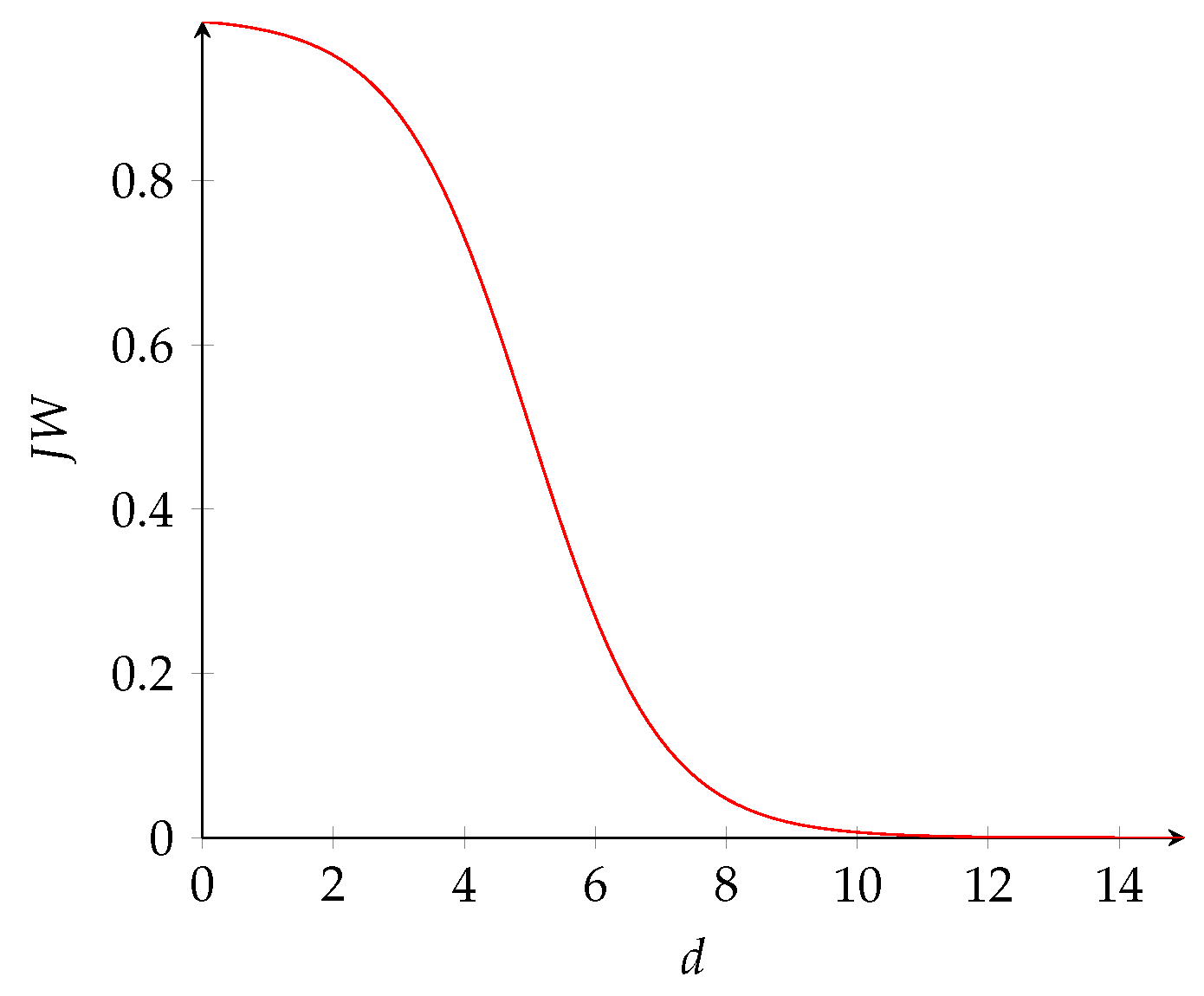
When we are traveling from one location on the road network to another, traffic jams at different distances from our location will have a different impact on the choice of route. Due to its monotonic, smoothing qualities, sigmod is frequently employed as an activation function for neural networks, automatically projecting variables between 0 and 1. Here, it is refined to analyze the effect of crowded roads on route planning and is expressed as the Equation (
3) named
(jam weight).
where
d specifies the distance between the road and vehicle and
represents a threshold within which the traffic status is important for route planning. The line graph for
is shown in
Figure 2. From
Figure 2, the value of
is relatively large when
d is close to 0, which means that the crowded road has a big influence on route planning. When
d exceeds the threshold
, it rapidly declines until it is very close to 0.
In the
model, for crowded roads, we add their influence on path planning to the road weight. After a series of experiments, the weight of roads in the road network is expressed as Equation (
4).
where
k implies the magnification,
d means the distance from the crowded road to the vehicle, and
denotes a road in the road network. It can be seen that when the congested road remains within the threshold
, a smaller value of
d means a larger value of
, which leads to a larger increase in road length. In addition, when
d exceeds the threshold
, the value of
will be close to 0 within a small interval of
d. At this time, the expansion to length of roads is also almost 0. This exactly satisfies our assumption of not considering the roads outside the threshold range. The roads have different weights for different vehicles, which are related to their distance from the vehicle.
In the model, the weight of roads is mainly affected by the road length and parameters
k and
. When the road is congested, it takes longer for vehicles to cross the road. Under the condition that the speed remains constant,
k is used to increase the length of the road to simulate the process. In the real road environment, the size of
k can be dynamically adjusted according to different jam levels, congestion time and so on. The result of Equation (
4) shows that the influence of
k on road weight is basically limited to the threshold
. When
d is larger than
, the c
gradually decreases to close to 0, and the influence of
k on road weight also gradually weakens.
is an important indicator of
, which represents the range of expected smooth roads. For city travel, the value of
should be relatively small to ensure smooth travel considering the rapidly changing traffic flow. However, for intercity travel, a larger
is preferable since we pay more attention to the overall travel status due to the longer travel distance.
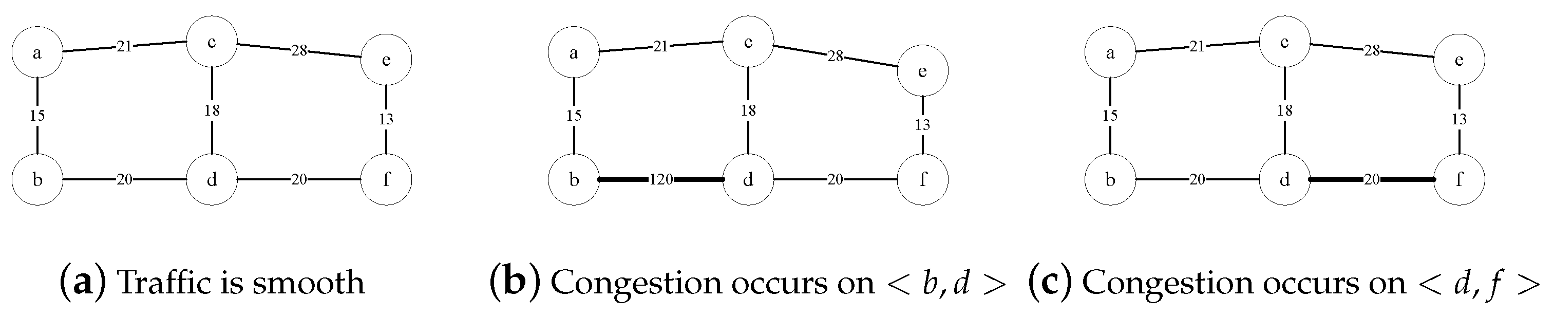
In the road network (unit: km) depicted in
Figure 3, the start and end are
a,
f, respectively. When the traffic state is free, the weighted road network is illustrated in
Figure 3a. We set
and
. When the
road becomes congested, according to Equation (
4), the weight of
is
, indicating that the congestion on road
has a greater impact on route planning. However, when the road
is congested, the weight is
. Clearly, the congestion has little effect on route planning. From
Figure 3, we observe that the road is far from the start a, which is why the current traffic situation on the road does not need to be taken into account.
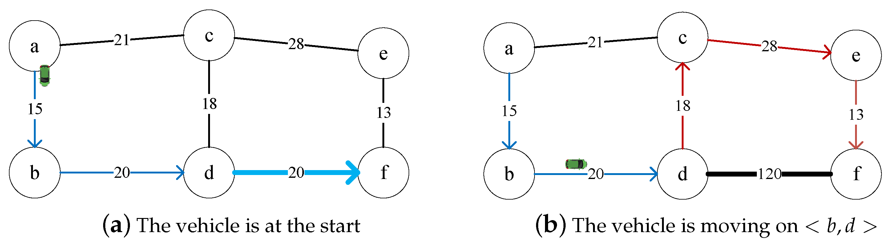
Figure 4 shows an example of route update using the data in
Figure 3, assuming that road
is congested.
Figure 4a displays the state of the road network when a vehicle is located at the start. According to Equation (
4), the actual weight of the
road at this time is still about 20 km. The optimal route is
, marked by the blue arrow in
Figure 4a. When the vehicle is driving on the
road, road congestion can be detected. If the road
is still congested, the algorithm reconstructs the road network according to Equation (
4). Suppose that the distance between intersection d and the vehicle is 15 km, and the weight of
will be 120 km which means that the optimal path for the vehicle is
indicated by the red arrow in
Figure 4b. On the contrary, if the state of road
is free at that time, the route update will not be carried out.
In this paper, the algorithm is utilized for path planning. Typically, in the algorithm, where signifies the actual cost of traveling from the start to the current, which is the sum of the cost from the start to the parent node and the cost from the parent node to itself. The estimated cost from the current position to the target point is represented by . The closer the node is to the end, the smaller the value of is, and the smaller the value of is. This ensures that the search progress towards the end if is maintained. The is the route planning method, and in this paper, the Euclidean distance is the heuristic function.
The model-based navigation algorithm can be represented as follows.
- 1.
VDWR model is generated based on the location of the vehicle and the current traffic data.
- 2.
While the vehicle is moving, the system automatically collects the road situation within the threshold .
- 3.
If jammed roads are detected, the model is automatically updated and the optimal path is recalculated.
4. Multi-Vehicle Dynamic Evacuation Algorithm Based on Route Diversity
There have been many studies on reducing urban congestion caused by traffic accidents, natural disasters, etc. An effective method for vehicle evacuation helps to reduce pressure on the road network and avoid traffic congestion. In our previous study [
14], we proposed a dynamic evacuation algorithm for multiple vehicles based on spatial diversity. However, as discussed in
Section 2.2, this method had some shortcomings. To overcome these issues, we present a new approach for multi-vehicle evacuation based on route diversity, which is detailed in this section.
First, we propose the concept of route coincidence (
), which represents the length of overlap part of the routes between vehicles. We assigned the route of vehicle
p to the ordered set
and the route of vehicle
s to the ordered set.
Then the route coincidence of vehicle
p and
s can be expressed as the Equation (
5).
where
,
R denoted the set of roads in the road networks.
The smaller the value, the less the trajectory overlap between vehicles, which means that the distribution of vehicles in space is more balanced, and the possibility of road congestion is low. Therefore, we first obtain travel routes based on before evacuating. Then, we give priority to the vehicle closest to the evacuation center. For the remaining vehicles, we calculate the for each vehicle. The vehicle with the smallest is evacuated first.
During an evacuation, however, traffic is often more congested on roads closer to the evacuation center than on those further away. Therefore, when we calculate the
, roads at different distances from the evacuation center are given different weights. We made the following improvements to the
in the Equation (
6).
As the number of vehicles increases, evacuation time tends to increase as well. Later vehicles tend to be less affected by the first evacuated vehicles since they are either far away from the evacuation center or have arrived at their destination. We sum all of the
between the current vehicle and all planned vehicles. It was written as the Equation (
7).
Then we average it to obtain Equation (
8).
In the above two equations, p represents the vehicles to be evacuated, and Q represents the set of already evacuated vehicles.
If two vehicles have the same but different distances to the evacuation center, we also need to consider their priority. In this case, vehicles have a higher priority if their destination is closer to the evacuation center. This is due to the fact that the vehicle whose destination is closer to the evacuation center has a shorter travel distance, causing less pressure on the road network.
Finally, based on the ideas presented above, we proposed the theory of route diversity, which is expressed as the Equation (
9).
where
denotes the route diversity between vehicle
p and already evacuated vehicles. A smaller
value indicates not only more diversity, but also a higher priority in evacuation planning.
denotes the distance from the destination of the vehicle to the evacuation center.
represents the maximum of
from all unplanned vehicles.
According to the theory of route diversity, when the value is higher, it indicates that the diversity of the route is smaller and the vehicle should have a lower priority in evacuation planning. As the evacuation progresses, the vehicles with greater time intervals between evacuations will have less impact on each other. When two or more vehicles have the same value, the vehicle with the closest destination to the evacuation center should be given higher priority as it will have a shorter travel time and less impact on the road network.
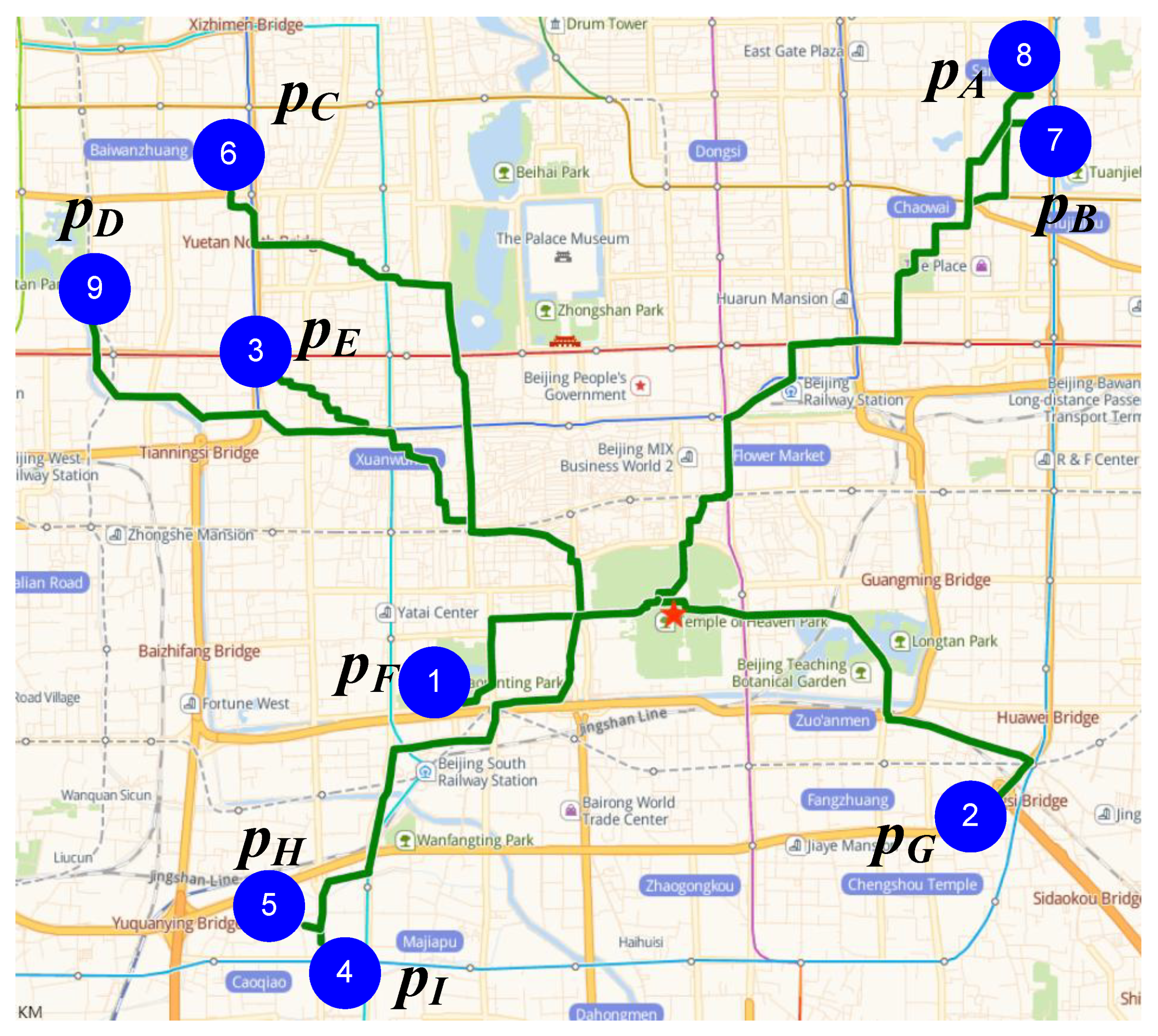
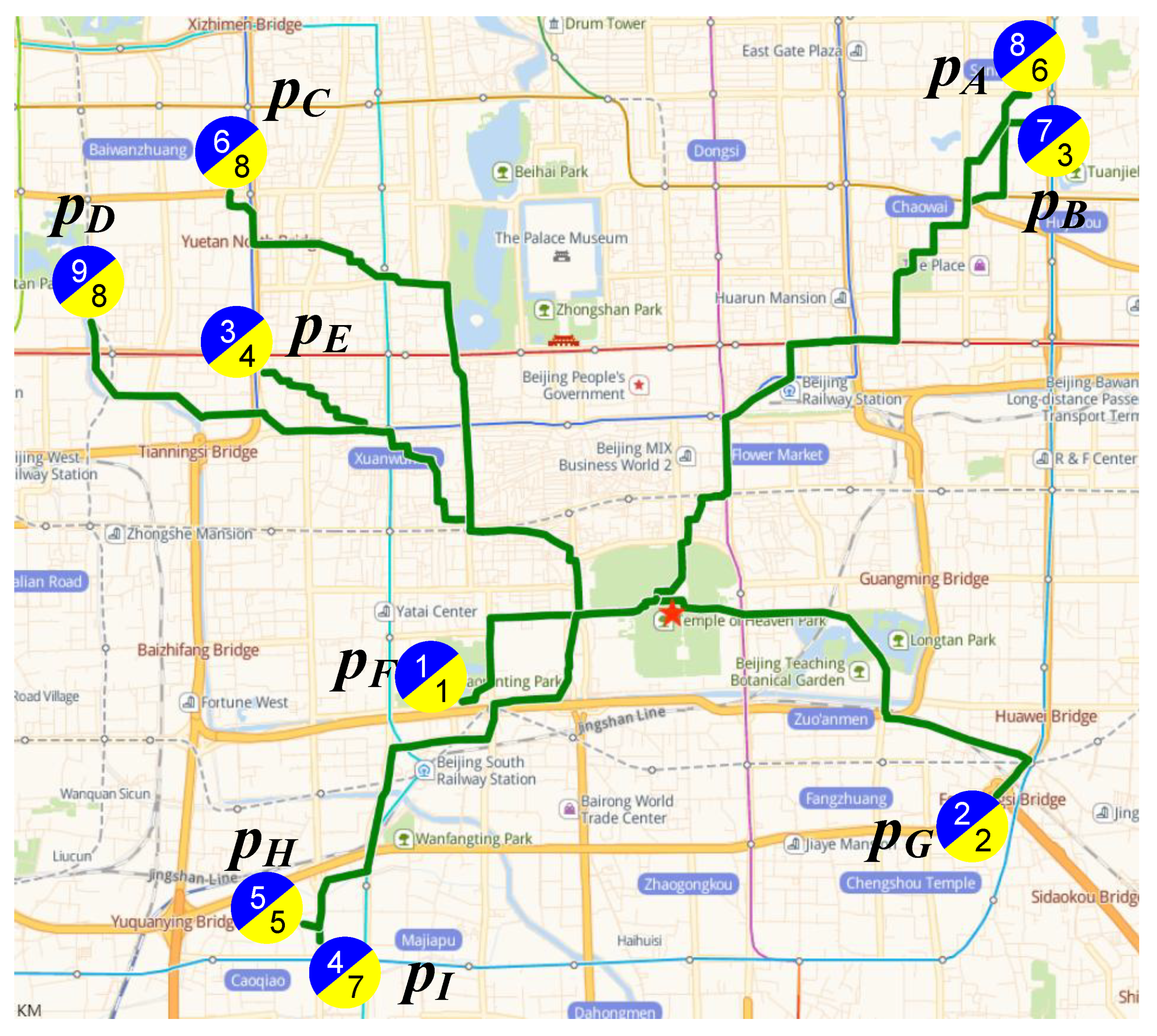
Using the nine positions in
Figure 1 as the vehicle ends, we conducted experiments based on route diversity theory again. The evacuation order is shown in
Figure 5, and the calculation process and selection of positions are shown in
Table 1. The number in the blue semicircle is the evacuation order based on the spatial diversity algorithm, while the number in the yellow semicircle represents the evacuation order based on our newly proposed route diversity algorithm.
According to the idea of route diversity, we first choose the position that is nearest to the evacuation center, which is the same as the idea based on spatial diversity. As a result, both algorithms select
first, as shown in
Figure 5. In
Table 1, the first row shows the distance of each position from the evacuation center. A big difference occurs at position
, which ranks seventh in the spatial diversity-based algorithm, but third in our algorithm. After the
, it can be seen from
Figure 5 that only the trajectories of the
and
do not overlap with the
and
. According to the Equation (
9),
is given higher priority because of its smaller distance from the evacuation center, as shown in the third row of
Table 1. For the remaining vehicles, we prioritized their evacuation orders according to the principle of route diversity.
In the following, we summarize the basic steps of the multi-vehicle dynamic evacuation algorithm based on route diversity.
- 1.
We obtain information on the evacuation center and vehicle routes.
- 2.
The evacuation order of vehicles was determined by the route diversity principle.
- 3.
According to the route information, we check the status of each starting road. If it is crowded, the vehicles wait. Otherwise, evacuation is performed.
- 4.
A single point navigation algorithm in
Section 3 is used to achieve the path planning of each evacuation vehicle.
Next, we introduce the algorithms used in the above process.
In Algorithm 1, we introduced how to arrange the order of evacuation of vehicles. Firstly, we define a set
to store vehicles to be evacuated (line 1). Then the vehicles are sorted by the distance between the end and the evacuation center, from smallest to largest (line 2). Then, we get the index of the next evacuated vehicle until the number of vehicles unplanned is 0 (line 3). First, if the
is empty (line 4), we select the vehicle closest to the center as the first. Then we add it to the already planned set
(line 5) and remove it from the unplanned set
(line 6). If the list is not empty, the next vehicle is selected according to
algorithm (line 9). Similarly, the selected vehicle is put into the already planned set
(line 10) while being removed from the unplanned set
(line 11). The algorithm will repeat this step until the set of unplanned vehicles is empty. Finally, we return the set of planned vehicles (line 14).
| Algorithm 1: DynamicEvacuation |
 |
Algorithm 2 is used to describe how to select the car with the smallest
every time. For each car to be planned (line 1), we first assign an initial value to its
(line 2). The value can be calculated by Equation (
7) (lines 3 and 4). Then, based on the previously calculated
, we get
(line 6). According to Equation (
9), we obtain the final calculation result (line 7), which is used to compare the route diversity between the current vehicle and all the planned vehicles. Then it is compared to the original calculated result (line 8). if the newly calculated
value is smaller, we save the result (line 9) and index (line 10). Finally, we choose the vehicle with the smallest
as our next vehicle to be evacuated (lines 9–12).
| Algorithm 2: GNP |
 |
Algorithm 3 is used to calculate the overlap of the routes between vehicles. We first obtain the routes of the planned vehicles and the unplanned vehicles (line 1 and 2). Then we get the minimum number of roads in the paths of the two vehicles (line 3). Next, we calculate the
between the vehicles based on Equation (
6) (line 5–8). Finally, we return the results of the calculation (line 9).
For specific vehicles in the evacuation process, we will use the navigation algorithm based on the
VDWR road network model for route planning. At the beginning of the evacuation process, the vehicle will follow the current planned route. During the drive, the navigation system will automatically detect traffic on the roads within the threshold
. When congestion is detected on the route, the algorithm will take the current position of the vehicle as the start and reconstruct the road network model considering current traffic data. When an alternative route is found using the current road network model, the navigation system will guide the vehicle to take this route to avoid congestion.
| Algorithm 3: computerUpdateRc |
 |
5. The Experimental Evaluations
In this section, we first introduce experimental settings and datasets. Then, we evaluate the effectiveness of our model and approach.
The experiments were conducted based on the road network data in Beijing. Due to the limitations of computer performance, we only matched the road network within the 3rd Ring Road of Beijing as the basis for the experiment, which contains 18,649 intersections and 24,360 roads. We store the intersections and roads in an array based on their position index, which allows us to obtain the status of each intersection and road in only time. Our computer’s processor is an Intel(R) Core(TM) i5-6500 CPU @ 3.20 GHz 3.20 GHz with 8.00 GB of RAM. Graphics card type is AMD Radeon(TM) HD8490.
5.1. Effectiveness of Model
In this section, we use the algorithm for route planning based on the model. Then we visualize the routes using the Gaode Map API to verify the benefits. We do not compare our algorithm with that of commercial navigation maps such as Google Maps, Baidu Maps, and AMAP since travel routes are closely related to traffic data, we cannot replicate the live traffic model.
In order to verify the effectiveness of the model, we visualize the route when the distance between the start and end is at different scales. We set and and the results are shown below.
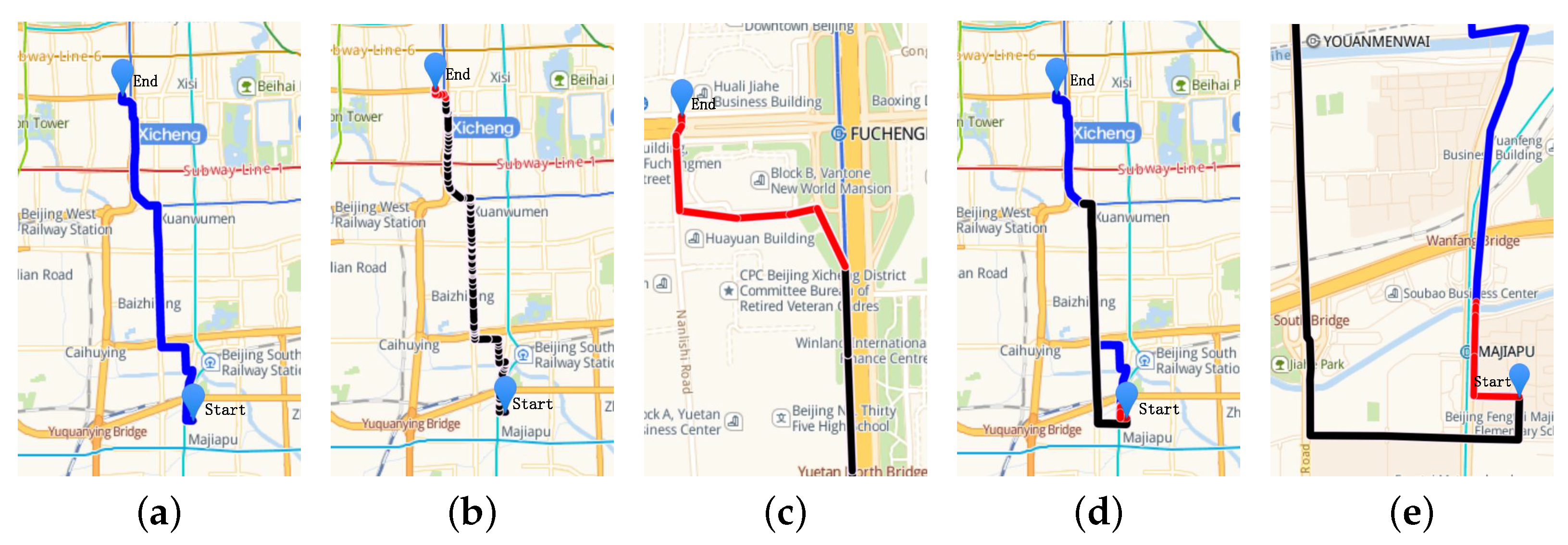
Firstly, two positions that are far apart were chosen as the start and end of the vehicle. The result is shown in
Figure 6. The blue line is the optimal route when the traffic is free, followed by the red line for crowded roads and the black line for the optimal route under jammed conditions. Next, we set roads near the end to be crowded, as shown in the red line in
Figure 6b. For the sake of observation, we zoom in on the crowded part, which is shown in the
Figure 6c. As can be seen, the black line completely covers the original blue line, which means that the route did not change after the jam occurred. In turn, we set the status of the roads near the start to crowded. The results are shown in
Figure 6d and the details are presented in
Figure 6e. It could be found that the black route, which is a novel optimal route designed by the
algorithm based on the
VDWR model, avoids the congested red road.
Then, two closer locations are chosen as the start and end for a vehicle. The experimental results are depicted in
Figure 7. At this time, we make the roads near the end crowded.
Figure 7b gives an overall overview, and the detailed information is shown in
Figure 7c. The figure shows that the
algorithm avoids crowded roads when the distance between the start and the end is short (the distance between them is close to the threshold
).
From a travel perspective, when the distance between the start and end is short, the travel time is usually less and there is less chance for significant changes in traffic data during that period. In such cases, the algorithm should consider the entire road network and avoid congested roads, even if they are close to the end.
According to the above experiment, we can see that the proposed model enables navigation algorithms to obtain suitable routes based on live traffic. Next, we will evaluate the search efficiency of the algorithm in terms of the model.
5.2. Efficiency of Model
To analyze the efficiency of the navigation algorithm under the model, we conducted an analysis focusing on the algorithm’s performance with respect to various metrics. Specifically, we analyzed the path length, the number of expanded nodes during planning, the time required for route planning, and the length of the optimal route.
Under initial conditions where all roads in the network are free, we used the algorithm to obtain the optimal route for vehicles. We then modified the status of different roads in the optimal route to “crowded”, based on their distance from the start. This allowed us to observe the algorithm’s performance under different traffic conditions. Specifically, we obtained routes for three scenarios: (1) smooth traffic, (2) traffic conditions under the VDWR-based model, and (3) Based on weighted road network (The road weight are calculated without considering the distance between congested roads and vehicles).
We first set the
, and choose a start
and an end
, where the distance between them is relatively short. Next, we simulate a scenario where the roads near the start of the route are congested while the rest of the road network is free. The results of this simulation are presented in
Table 2.
From the table, it can be observed that when traffic is free, the number of nodes to be searched is the smallest, and the distance is the shortest. However, when road conditions are considered, the weight of congested roads increases, resulting in an increased number of nodes to be expanded. As a result, the final route obtained is longer than the optimal route.
Further, these roads, which are close to ends, are set to be congested. The experimental results are shown in
Table 3.
When the distance between the start and the end is relatively short, the routes obtained through the model are guaranteed to be optimal under congestion avoidance, as confirmed by our experiments. This is because the short distance is also close to the threshold value of that we set, which is 3 km, and the total length of the route is also approximately 3 km. In such cases, the possibility of significant changes in live traffic is low, and the algorithm should consider the real-time status of roads to select the most optimal route. Our proposed model effectively meets this need, allowing navigation algorithms to obtain the most suitable routes based on live traffic data.
Next, we selected a pair of distant points as the vehicle’s start and end, with the start
and the end
10,000. We conducted the same experiment again and found that when the congested roads were located near the start, the results were basically the same as when the distance between the start and end points was short. Therefore, we focused on analyzing the situation when the congested roads were located near the end. The results of this experiment are shown in
Table 4.
From the above table, it is evident that the number of nodes and the distance of the route obtained based on the model are the same as those obtained under free traffic conditions. This implies that the algorithm fails to avoid congested roads. Moreover, the time and space required by the algorithm are also less than that required by the weighted road network. However, from the perspective of daily travel, it is not practical to consider road conditions that are 10,000 m away from the vehicle’s starting point.
Based on the previous discussion, it is clear that the route planning method utilizing the model achieves the global optimum when the distance between the start and end points is relatively short. This approach ensures a smooth driving process for the vehicle throughout the route. However, for longer distances, the algorithm based on the model considers only the road status within the threshold , disregarding traffic conditions beyond it. By doing so, the efficiency of path planning is improved.
5.3. Evaluation of Multi-Vehicle Dynamic Evacuation Efficiency Based on Route Diversity
In this section, we will evaluate the performance of the vehicle evacuation algorithm based on route diversity. To highlight its advantages, we will compare it with the evacuation algorithm based on spatial diversity [
14].
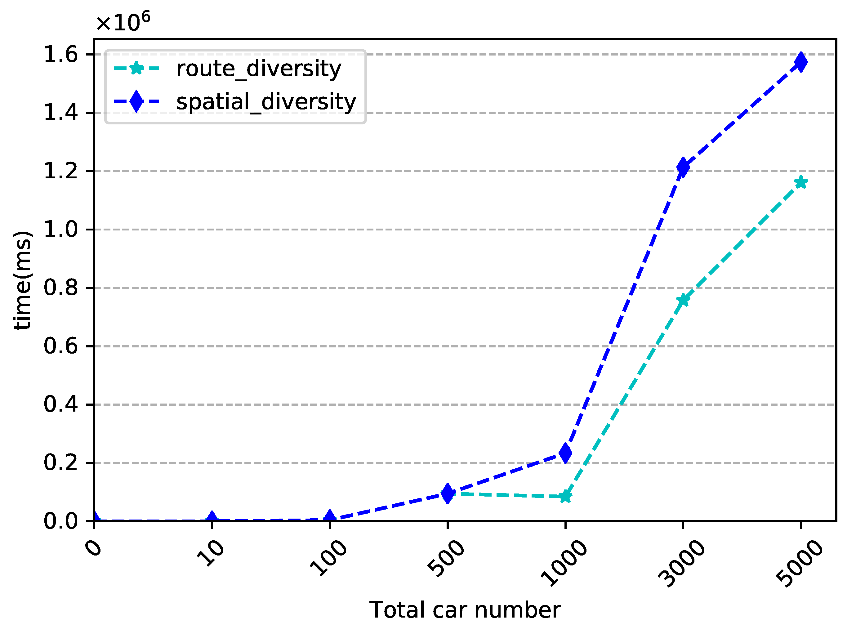
The purpose of this experiment is to evaluate the efficiency of the evacuation algorithm. The metric used for this evaluation is the time elapsed between planning the first vehicle and the last vehicle. Prior to evacuating a vehicle, we obtain the traffic status of the first road in its route. The vehicle will not be evacuated until the road is clear.
We selected evacuation center
and randomly generated destinations for the vehicles, in order to observe the evacuation effect of the algorithm at different scales, including 10, 100, 500, 1000, 3000, and 5000 vehicles. To evaluate the evacuation effect of the algorithm, we compared the results with the evacuation algorithm based on spatial diversity [
14]. To ensure the accuracy of the results, the destination of the vehicle is kept the same when comparing different algorithms at the same scale. The experimental results are shown in
Figure 8.
The data presented in
Figure 8 clearly show that the evacuation time increases as the number of vehicles to be evacuated increases. When only 10 vehicles are involved, there is little difference in the evacuation time between the two algorithms. However, as the number of vehicles increases, the difference becomes more significant. When evacuating 1000 vehicles, the time required by our new algorithm is less than half of that required by the original algorithm proposed by Cai et al. [
14]. This difference continues to increase as the number of vehicles to be evacuated increases. These results indicate that our algorithm outperforms the previously proposed algorithm [
14] in terms of evacuation time.
5.4. Evacuation Simulation Case Study
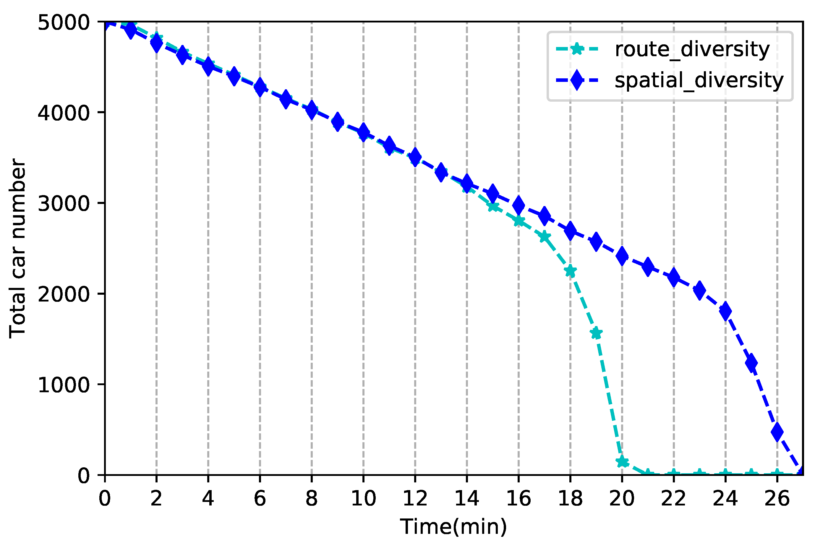
To visually demonstrate the superiority of our newly proposed multi-vehicle evacuation algorithm based on route diversity, we take the time of evacuating the first vehicle as the start and record the number of vehicles remaining at the evacuation center every 1 min. The results are then compared with those obtained using spatial diversity-based algorithms [
14]. The number of vehicles involved in the experiment is 5000, and the results are presented in
Figure 9.
The horizontal axis in the
Figure 9 shows the time interval between the current time and the start time of evacuation in minutes, while the vertical axis shows the number of vehicles remaining at the evacuation center. The curves represent the trend of the number of vehicles remaining at the evacuation center over time using the evacuation algorithm based on spatial diversity [
14] and the route diversity, respectively. The slope of the curves reflects the efficiency of vehicle evacuation. By comparing the curves, it can be observed that the efficiency of evacuation is roughly the same for both algorithms at the beginning of the evacuation. However, as the number of vehicles to be evacuated decreases, the algorithm based on route diversity reaches the inflection point of evacuation more quickly. Thereafter, it maintains higher evacuation efficiency than evacuation algorithm based on spatial diversity. Moreover, the newly proposed algorithm completes the evacuation 6 min earlier than the spatial diversity based algorithm [
14]. In conclusion, our newly proposed algorithm has better evacuation performance.
Based on the above experiments, we randomly selected 10 cars and observed their positions every 4 min from the evacuation start time. Again, we compared with the evacuation algorithm based on spatial diversity [
14]. Since we did not have the specific latitude and longitude information of the vehicles, we used the location of the intersection at the exit of the road where the vehicle was located instead. The results are shown in
Figure 10.
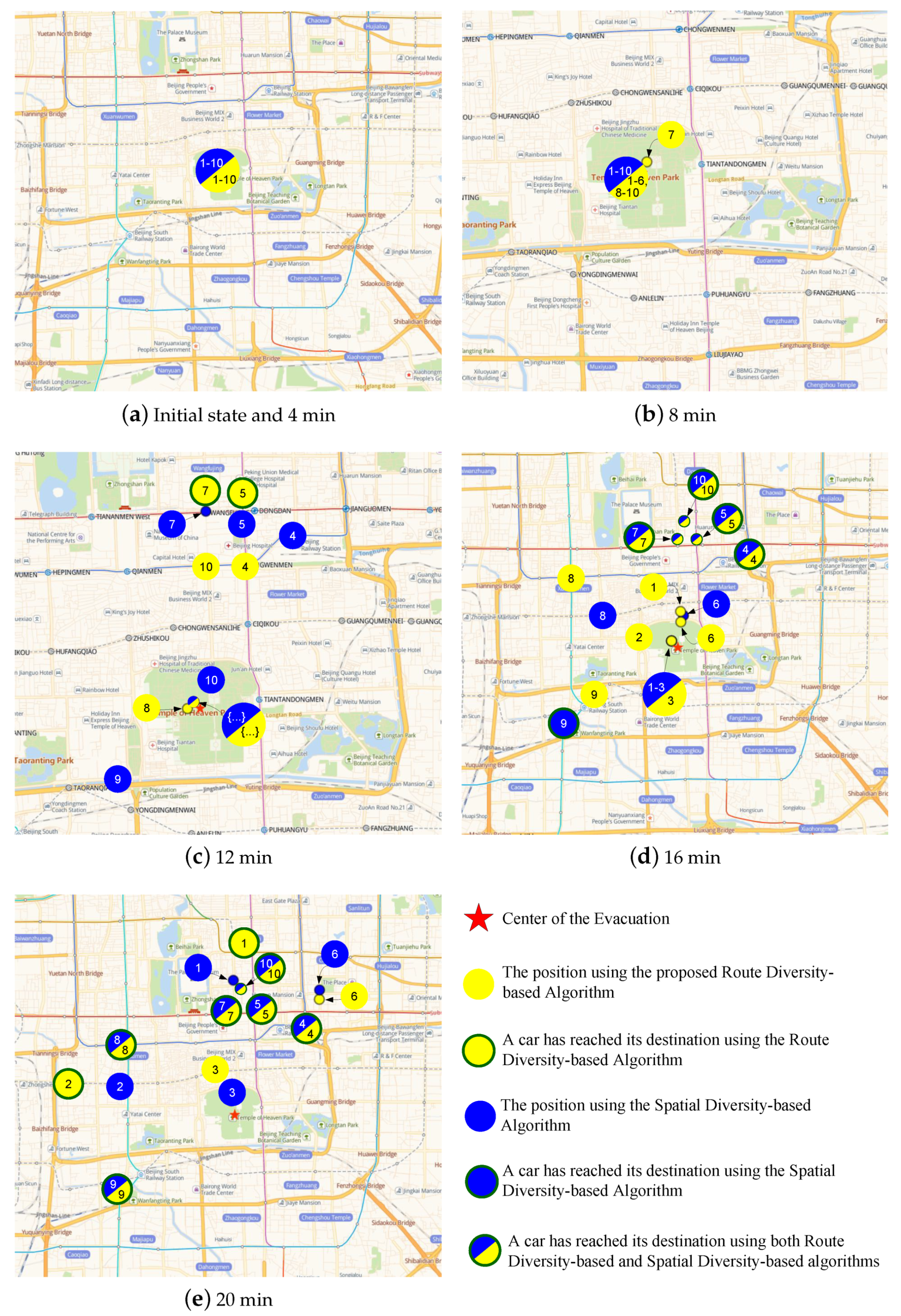
In
Figure 10, the yellow and blue circles represent the real-time position of the vehicles based on the route diversity algorithm and the spatial diversity algorithm [
14], respectively. The digits in the circles indicate the number of the vehicle. A green ring around a vehicle indicates that it has reached its destination. The pentagram represents the evacuation center.
In the 4 min of the evacuation, none of the selected vehicles had started evacuating, as shown in
Figure 10a. At 8 min into the evacuation, as shown in
Figure 10b, vehicle 7 has already departed using the route diversity algorithm, while none of the vehicles have started evacuating yet using the spatial diversity algorithm. At the 12 min, as shown in
Figure 10c, two of the 10 selected vehicles have already reached the end using the route diversity algorithm, but none of them have reached their destination using the spatial diversity algorithm. The evacuation order between the two algorithms is also different. For example, in the route diversity algorithm, car 8 has priority over car 9, while the order is different in the spatial diversity algorithm.At the 16th minute of the evacuation, illustrated in
Figure 10d, the route diversity algorithm has successfully evacuated 9 out of the 10 selected vehicles, and 4 of them have reached the end. In contrast, using the spatial diversity algorithm, 5 vehicles have reached their destination, and only 2 of them are still moving. Finally, in
Figure 10e, the positions of the vehicles after 20 min from the start of the evacuation are shown. The route diversity algorithm has enabled 8 out of the 10 selected vehicles to reach the end, whereas only 6 vehicles have reached the end using the spatial diversity algorithm. As a result, the newly proposed evacuation algorithm demonstrates superior performance compared to the spatial diversity-based evacuation algorithm.


