Abstract
With the rapid development of the big data era, Unmanned Aerial Vehicles (UAVs) are being increasingly adopted for various complex environments. This has imposed new requirements for UAV path planning. How to efficiently organize, manage, and express all kinds of data in complex scenes and intelligently carry out fast and efficient path planning for UAVs are new challenges brought about by UAV application requirements. However, traditional path-planning methods lack the ability to effectively integrate and organize multivariate data in dynamic and complicated airspace environments. To address these challenges, this paper leverages the theory of the three-dimensional subdivision of earth space and proposes a novel environment-modeling approach based on airspace grids. In this approach, we carried out the grid-based modeling and storage of the UAV flight airspace environment and built a stable and intelligent deep-reinforcement-learning grid model to solve the problem of the passage cost of UAV path planning in the real world. Finally, we designed multiple sets of experiments to verify the efficiency of the global subdivision coding system as an environmental organization framework for path planning compared to a longitude–latitude system and to demonstrate the superiority of the improved deep-reinforcement-learning model in specific scenarios.
1. Introduction
Unmanned Aerial Vehicles (UAVs) play an important role in many fields, such as aerial photography, disaster rescue, power inspection, etc. [1]. No matter what field it is used in, a user’s basic requirement of their UAV that allows it to perform tasks is for it to be able to find a sequence of points or a continuous polyline from a starting point to an end point; such a sequence of points or polylines is called a path from the start point to the end point. This kind of strategy of selecting an optimal or better flight path in the mission area, with reference to a certain parameter index such as the shortest flight time consumption or the lowest work cost, is called UAV path planning [2].
In the context of the big data and information age, the operational environment for drones is becoming increasingly complex, particularly in low-altitude airspace below 1000 m. There are not only UAVs and static targets in this airspace but also other moving entities, such as civil aircraft and birds [3,4]. Additionally, electromagnetic and radar fields may also be present [5,6,7], posing potential threats to UAVs. The complexity of the UAV path-planning scenario translates into data complexity, with diverse data sources and organization methods. Massive, multivariate, and heterogeneous data in the absence of a unified organization method are difficult for drones to handle, and it is difficult to carry out unified management and expression. UAV path planning requires traversing an entire map to select an optimal path [8]. Since UAVs have to consider factors such as battery life and safety during flight, it is necessary to consider the cost of passage to make a balanced choice between the length of a path and safety [9,10]. According to research, the application of UAVs in civilian fields has expanded to nearly a hundred different areas [11], and the trend towards increasingly complex scenarios and diversified purposes is evident. Therefore, it is crucial to study intelligent UAV path-planning methods in complex environments.
There are three main types of existing path-planning environment frameworks: local single-scale grid systems [12,13], longitude–latitude systems [14,15], and global subdivision grid systems [16]. Both the local single-scale grid systems and the longitude–latitude systems have had early applications and represent traditional path-planning environmental frameworks. The local single-scale grid systems are similar to grids [17], but they are not identical. These systems’ advantage is in their relatively straightforward modeling process courtesy of their localized and single-scale nature. This simplicity has made them popular for path planning in simulated environments. However, the local system requires the establishment of a new local grid coordinate system based on the real environment each time the path-planning algorithm is applied in real-world scenarios. Consequently, this process consumes time and resources. On the other hand, the longitude–latitude system is fundamentally a vector description, essentially describing objects through a series of connected points. If sampling is sufficiently detailed, this system can effectively describe obstacle contours. An airspace environment as described by a longitude–latitude system is typically obstacle-free, with any point in the entire environment being reachable unless it is an obstacle. Yet, this system has difficulty describing regional characteristics, especially geospatial elements within geographic characteristics. In summary, local single-scale grid systems and longitude and latitude systems are inefficient when serving as environmental organization frameworks for path-planning problems. Moreover, vector descriptions can be computationally complex and time consuming when performing UAV path-planning tasks. The global subdivision grid system is founded on dividing the earth’s global space into adjustable grids, constituting a global and multi-scale grid system. The path-planning environment’s raster and vector data can both be stored and organized in this system, aligning with the data’s spatiotemporal attributes. Consequently, the global subdivision grid system can be considered a more advanced form of data organization, especially when solving problems that require environmental discretization. It is worth mentioning that the global subdivision grid system is not so suitable for solving vectorization problems. Existing path-planning methods, such as the classic A* algorithm [2], are best-first searches, meaning that they are formulated in terms of weighted graphs: starting from a specific starting node of a graph, they aim to find a path to a given goal node with the smallest cost (least distance travelled, shortest time, etc.). They execute this by maintaining a tree of paths originating at the start node and extending those paths one edge at a time until the specified termination criterion is satisfied. They primarily considers feasibility (obstacle avoidance) and distance factors (securing the shortest distance while bypassing obstacles). These algorithms struggle to incorporate airspace traffic costs during flight and, consequently, cannot balance a UAV’s choice between flight distance and safety. How to incorporate the traffic cost into the consideration of the loss function is a scientific issue that interests many researchers [9].
These algorithms rely on the excellent feature representation ability of deep neural networks, the self-supervised learning ability of the reinforcement learning agent, and powerful high-dimensional information perception, understanding, and nonlinear processing capabilities. They are model-independent and suitable for location environment decision-making problems. Though deep reinforcement learning (DRL)’s development began in the late 1980s, it was not until 2009 that scholars combined the Q-Learning algorithm with drone applications. Q-learning is a model-free reinforcement learning algorithm used to determine the value of an action in a particular state. It does not require a model of the environment (hence being “model-free”), and it can handle problems with stochastic transitions and rewards without requiring adaptations. Donghua and others [18] proposed a flight-path-planning algorithm based on the multi-agent Q-Learning algorithm. However, traditional reinforcement-learning algorithms, constrained by their strategy representation ability, could only tackle simple, low-dimensional decision-making issues. The introduction of deep reinforcement learning broke this limitation, with Mnih et al. [19,20] combining a Convolutional Neural Network and Q-Learning to craft the DQN algorithm model for visual-perception-based control tasks. Rowell et al. [21] designed a reward function of the DQN algorithm model to increase rewards and punishments based on multi-objective improved distance advantage, function rewards, no-fly penalties, target rewards, and route penalties. UAVs trained using the DQN algorithm demonstrated superior threat avoidance, real-time planning, and reliable route generation prowess compared to traditional obstacle avoidance algorithms. However, most of the current schemes that incorporate the traffic cost into the loss function have improved this classic algorithm. Jun et al. used the Bellman–Ford algorithm to make a balanced choice between distance and safety in a complex environment considering the safety of UAVs [9]; Wei et al. made improvements to the A* algorithm so that UAVs could consider more factors in path planning [10]. Shorakaei et al.’s work represents a significant effort in refining path-planning methods for UAVs [22]. They adopted Jun et al.’s definition of traffic cost and improved genetic algorithms. Their improvement made to the algorithm was the consideration of traffic cost, a critical aspect often overlooked in traditional approaches. In their approach, instead of exclusively focusing on the shortest path or simplest route, the factors of potential traffic within an airspace and safety factors were also considered. The result was a more balanced and realistic path for UAVs that, while being potentially slightly longer or more complex, minimizes the risk of collisions or other safety issues. This is a testament to how novel algorithms and strategies, combined with traditional principles, can pave the way for safer, more efficient UAV operations. Yet, the full potential of deep reinforcement learning in such scenarios remains largely untapped, inviting further exploration in future work.
In summary, classic path-planning algorithms (such as A*) and non-learning-based intelligent algorithms (such as genetic algorithms) have been applied to task scenarios that consider traffic costs; however, the research field of combining deep-reinforcement-learning-based path-planning methods with task scenarios that consider traffic costs has not yet been fully explored. Therefore, to address both the inefficiencies of traditional environmental organization frameworks and problems in data association and representation, such as those relating to single-scale grid systems and latitude and longitude systems, we chose the global subdivision grid system. As it is a typical representative of the global subdivision grid system and due to its unique segmentation method and coding rules, GeoSOT (geographical coordinate grid subdivision by one-dimension-integer and two to n th power) [23] can effectively serve as an environmental organization framework for path-planning problems. This paper proposes a GeoSOT-based modeling method. Building upon this, a deep-reinforcement-learning grid model was constructed, incorporating passage cost in the reward mechanism to realize UAV path planning in complex scenarios in which passage cost is considered. It would be valuable to include a comparison with other baseline algorithms commonly used in UAV path planning, such as A*.
The main unique contributions of this paper are as follows:
- In the context of the intelligent development of UAVs and industries, in view of the inefficiency of the traditional environmental organization framework, the difficulty of data association and expression, and the consideration of traffic costs in UAV path planning, a set of deep-reinforcement-learning grid models with a unified global space framework was established.
- Building upon the GeoSOT global subdivision coding model and local location recognition system, we introduce a modeling method grounded in an airspace grid. Additionally, the low-altitude airspace environment and dynamic targets of UAV flight are gridded and encoded so that the gridded airspace environment data can be better stored and managed.
- The Nature DQN algorithm is integrated to devise a specialized application method tailored to specific scene requirements, including reinforcement learning framework construction, neural network model construction, reward mechanism improvement, etc. This culminates in the design of a path-planning experiment for specific application scenarios to validate the robustness of the model and its superiority over classical algorithms in typical scenarios.
The remainder of this paper is organized as follows: The second section elucidates the method employed, and the third section describes a typical experiment conducted on the deep-reinforcement-learning grid model, which was mainly based on the model’s principle and the improved method proposed above, in order to carry out a relatively sufficient application verification experiment. Finally, we conclude our findings and suggest potential directions for future research.
2. Materials and Methods
The overall architecture of the deep-reinforcement-learning grid model includes a demand layer, an input layer, a processing layer, and an output layer. It is a relatively complete model system, as shown in Figure 1 below.
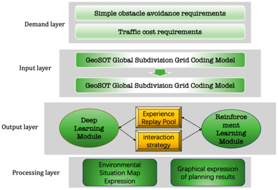
Figure 1.
An overall architectural diagram of the model.
The first layer of the model is the demand layer. Users need to clarify the specific scenarios and related requirements of the UAV path-planning task. The second layer is the input layer. This paper uses the GeoSOT global subdivision grid coding model to construct various data in the environmental module. The third layer is the processing layer, which produces results through the linkage cycle of the deep learning module and the reinforcement-learning module. The fourth layer is the output layer, which outputs the corresponding path-planning results.
2.1. Environment Modeling
For all kinds of data in complex scenes, this paper proposes an airspace gridded-environment modeling method, which was established based on the three-dimensional subdivision framework of earth space. It is a model for data organization in and the calculation and expression of the airspace environment where UAV missions are located.
Relying on the basic theory of earth space three-dimensional subdivision grids, grid modeling was carried out for the airspace environment of UAV flight. The core idea of this process is to divide and encode the airspace environment of drones in a seamless and non-overlapping grid to build a three-dimensional grid map of the airspace.
2.1.1. Airspace Grid Basics
The airspace grid is a three-dimensional subdivision grid system developed with a focus on aerial vehicle applications. It is fundamentally based on GeoSOT-3D, a three-dimensional earth space subdivision grid. It primarily spans from the ultra-low-altitude flight environment to the ultra-high-altitude flight environment for UAVs, with an altitude range extending from the ground surface up to a height of 20 km above the ground.
GeoSOT is a 2n one-dimensional integer array geographic coordinate global subdivision reference grid [23]. This grid system, which falls under the category of longitude–latitude subdivision grid systems, was proposed by the team led by Cheng Chengqi at Peking University. It is shown in Figure 2 below.
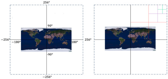
Figure 2.
A schematic diagram of GeoSOT subdivision grid.
Within this system, grids at levels 0–9 are degree-level grids, those at levels 10–15 are minute-level grids, and those at levels 16–21 are second-level grids. When all grids are subdivided down to the 32nd level, the resultant grid size is (1/2048″) × (1/2048″). Through the aforementioned divisions, the GeoSOT grid obtains advantages that include multi-scale consistency in time and space and unique global subdivision. This grid is flexible and expandable and allows for expedited analyses and applications within the field of two-dimensional environments.
GeoSOT-3D is built upon the foundational GeoSOT but extends its utility via incorporating height-dimensional information. This enhanced model maps height to and thereby corresponds to an airspace range that stretches from 50,000 km above the Earth’s surface to its center. As such, GeoSOT-3D can be applied to scientific research fields that necessitate height information, like UAV path planning [24].
The two-dimensional subdivision grid (GeoSOT) has a mapping relationship with the three-dimensional grid (GeoSOT-3D). When the height dimension is set to 0, the three-dimensional grid can be transmuted into a GeoSOT grid. By introducing height information, GeoSOT-3D is able to construct a multi-scale octree grid, as shown in Figure 3.
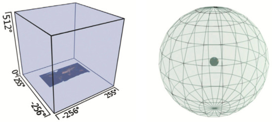
Figure 3.
A schematic diagram of Geosot-3D [25].
An octree is an efficacious data structure that partitions a three-dimensional data grid set into varying bounding volume levels. Through this type of division, each subdivision voxel aligns with a unique spatial position and its corresponding spatial information, thereby creating seamless and non-overlapping spatial coverage.
Once GeoSOT-3D executes grid subdivision, a grid code is utilized to establish the spatial position of the grid. Grid coding primarily involves four types of encoding: binary 3-dimensional coding, binary 1-dimensional coding, decimal 3-dimensional coding, and octal 1-dimensional coding [25].
Among these, octal 1-dimensional encoding is applied to the octree index; binary 3-dimensional encoding is separately encoded in the three dimensions of longitude, latitude, and height; and binary 1-dimensional encoding is an integration of binary 3-dimensional encoding.
This model primarily adopts the encoding methods of binary 1-dimensional encoding and binary 3-dimensional encoding. The specific coding structure is shown in Figure 4.
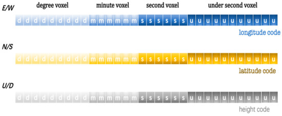
Figure 4.
A diagram of the binary three-dimensional coding structure.
In the given figure, the first digit of the longitude code denotes east or west longitude, the first digit of the latitude code signifies southern or northern latitude, and the first digit of the altitude code indicates above ground or underground. The dimensions are then converted into binary numbers according to degrees (8 digits), minutes (6 digits), seconds (6 digits), and periods less than seconds (11 digits).
The binary 1-dimensional code merges the longitude, latitude, and altitude from the binary 3-dimensional code. This fusion process employs “Z” ordering, which is a crisscross combination of three-dimensional codes. This method helps circumvent low query efficiency that can arise when a certain dimension takes high priority during queries posed to a track-planning database. The figure provided below illustrates the GeoSOT-3D space-filling curve and space ‘Z’ sequence encoding (Figure 5).
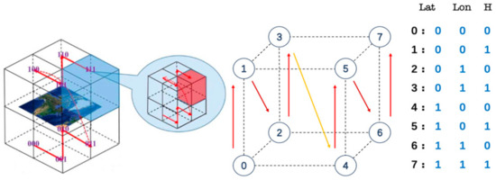
Figure 5.
GeoSOT-3D coding diagram.
The structure of the full binary 1-dimensional code after being encoded can be seen in the figure below. Its length is three times that of the single-dimension length in the binary 3-dimensional encoding structure. In the later stages of path planning, this binary 1-dimensional code will function as the primary key for querying the airspace grid database, acting as the certification entity for the database documentation, storing all the necessary information about the airspace environment, including obstacles and drone details, as shown in Figure 6.
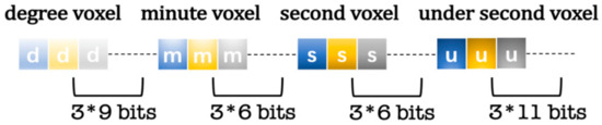
Figure 6.
The schematic diagram of binary one-dimensional encoding.
The GeoSOT-3D global subdivision reference grid offers global unity and multi-level capabilities, enabling the seamless division of global airspace without overlapping space. Simultaneously, it establishes a multi-level environmental grid within an airspace, which facilitates path planning and actual flight for various types of UAVs. Utilizing the GeoSOT-3D grid model eliminates the complexity of physical space concepts, accurately defines and divides obstacle boundaries, and enables rapid environmental modeling.
2.1.2. Environment Modeling and Mesh Coding Based on GeoSOT-3D
Based on the global subdivision reference grid system, the entire Earth’s space can be divided into multiple seamless and non-overlapping subdivision voxels, where each voxel serves as a grid in space. For the representation of UAV airspace environments, this paper refers to each subdivision unit, following the airspace’s subdivision, as an airspace grid. Relying on the GeoSOT-3D framework, spatiotemporal subdivision modeling of airspace environments primarily adheres to the following principles:
- Accuracy correspondence—Different UAV applications require different research scales. Hence, when subdividing and expressing spatial objects within an airspace environment, an appropriate subdivision level should be selected to match the research scale, i.e., the correct airspace grid accuracy should match the research accuracy.
- Lossless Expression—The representation of spatial objects in an airspace using spatiotemporal grids should result in a grid set that can fully contain the spatiotemporal range actually covered by the spatial objects. During representation, it is permissible to have redundant regions caused by using spatiotemporal voxels to depict detailed edges. Still, any omission of spatial or temporal regions corresponding to a given object, resulting in the loss of part of the spatiotemporal information, is not allowed [26].
- Simplified representation—While ensuring lossless expression, the spatiotemporal grid geometry used to represent objects in the airspace environment should be as simple as possible. The number of spatiotemporal grids should be minimized within the allowable range of error.
When subdividing the low-altitude airspace environment, all static low-altitude airspace objects can be composed of one or more airspace grids. The grid representation of low-altitude airspace objects essentially uses the airspace grid as the basic unit to model the spatial objects in the low-altitude airspace environment at a certain longitude. And any fundamental airspace grid at the same level does not overlap. The grid representation of any spatial object can be expressed using the following Formula (1):
In the provided formula, Area3 represents any three-dimensional spatial object, and ui and uj represent the basic airspace grid. Therefore, the formula suggests that any three-dimensional spatial object, Area3, can be represented by n basic airspace grids, and the intersection of any two airspace grids is null.
Based on the above foundational formulas, spatial objects in the low-altitude airspace environment can be expressed. Spatial object areas in the low-altitude airspace environment include both the airspace that drones can traverse and the space occupied by impassable obstacles. The steps for expressing a spatial object in the low-altitude airspace environment are as follows:
- Step 1—Determine the subdivision level.
- Step 2—Calculate its minimum outer bounding rectangle combination (MBR) based on the corner point coordinates of obstacles in the low-altitude airspace.
- Step 3—Carry out grid division for the target airspace according to the selected level. As long as part of the airspace grid contains obstacles, it will be marked as occupied.
When performing obstacle grid modeling, a crucial principle to follow is that all obstacle information should be retrievable. This requires that when determining the boundary and entering grid information, especially in the low-level grid airspace, as long as the grid contains obstacle information, it should be classified as a grid storing obstacles. Obstacle meshing is shown in Figure 7 [27].
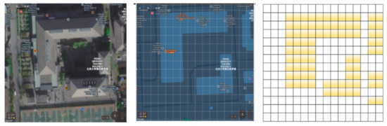
Figure 7.
The schematic diagram of low-altitude airspace environment grid expression.
When a UAV is performing a mission, as a dynamic object, it is necessary to consider the UAV location within the grid. When performing UAV flight missions in large-scale environments, in most cases, the physical attributes of the UAV can be ignored. Instead, more attention should be paid to the drone’s flight path on a macro level. At this point, the drone’s center of mass is typically considered the actual position of the drone. At each grid level, the grid where the drone is located is the grid where the center of mass can be found. UAV meshing is shown in Figure 8.
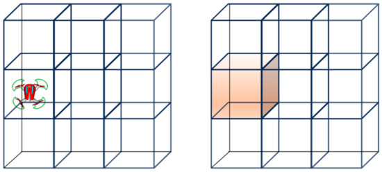
Figure 8.
The UAV grid representation.
The subdivision grid level usually selected is higher when UAVs perform missions, resulting in a longer code length. This can consume considerable storage space and reduce modeling speed. Given that the GeoSOT-3D grid adopts the recursive subdivision of the octree, the coding of the same grid voxel in different location identification systems also has a specific nested relationship.
Specifically, any grid (included in the local grid location identification system level 0 block GridLocal−0) under the local grid location identification system has its code within the global grid position identification system used as a prefix to form the code grid under the global grid position identification system, as shown in Figure 9.
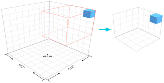
Figure 9.
The schematic diagram of octree subdivision of local grid position identification system.
Similarly, given the code of the grid under the global grid position identification system, it is only necessary to cut off the code of the 0-level block under the global grid position identification system from left to right, and the remaining codes are the codes of the grid under the local grid position identification system, as shown in Formula (2) below.
In the formula, represents the function assigning unique grid codes to individual subdivided three-dimensional cells, or “voxels”, within the global grid position identification system. The function () concatenates these codes in a head-to-tail fashion. , on the other hand, represents the code pertaining to the subdivided voxel within the local grid position identification system [28].
The use of a local grid position identification system facilitates code length compression, culminating in the formation of a “short code” within the local space, effectively enhancing query update efficiency. When a complete grid code is necessary, the 0-level voxel code can also be retrieved from the database and appended to the “local grid code”.
2.2. Deep-Reinforcement-Learning Grid Models
2.2.1. Fundamentals of Deep Reinforcement Learning
In 2013, the team at DeepMind introduced a novel method of deep reinforcement learning: Deep Q-Learning. Traditional Q-Learning algorithms work with discrete action spaces and state spaces, leveraging a Q Table to calculate state values and action values [27]. However, convergence tends to be challenging when the state space is large, and an excessive search space can consume significant memory resources. In light of the above, the DeepMind team made enhancements to the Q-Learning algorithm. Notably, they have incorporated an experience replay mechanism and employed a neural network to generate the Q value for performing different actions in each state. These implementations have compensated for the drawback of increased memory consumption typically associated with such expansive tasks.
Despite the algorithm’s impressive performance in Atari games, it suffers from certain limitations. The computation formula for the target Q value used in DQN is shown in Formula (3):
The calculation of the target Q value here uses the calculated by using the Q network parameters to be trained in the current stage, but in fact, the intention was to update the Q network parameters through yj. Nevertheless, the interdependence and consequent influence of these two components mean that there is a strong correlation between the current Q value and the targeted Q value. This poses an obstacle to the algorithm’s convergence. Therefore, Mnih presented an enhanced version of DQN; it was published in “Nature”, leading to the algorithm being commonly referred to as “Nature DQN”. This version nudges a step beyond DQN, elevating the target network and curtailing the dependence between the target Q value’s computation and the Q network’s parameters to be updated with a dual network structure. As a result, it significantly boosts the DQN algorithm’s stability. The algorithm flow chart of Nature DQN is shown in Figure 10 below [20].
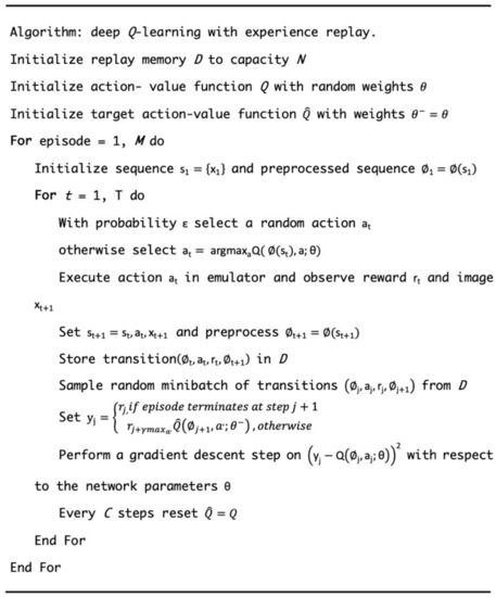
Figure 10.
The algorithm flow chart of Nature DQN [20].
The target action value function depicted is the so-called target network. Its introduction serves to bolster the stability of deep-reinforcement-learning training. To better grasp the significance of the target network, yj in the algorithm can be construed as a label in supervised learning. If the conventional DQN algorithm is employed, for the same quadruple data, the label would evolve with time step t. However, incorporating the target network entails that the label remains static over a period of time steps, denoted as t. This facilitates supervised learning from experiential labels, thereby enhancing neural network training stability. In summary, freezing the target for a duration aligns better with supervised learning from labels as opposed to labels that fluctuate with each time step. This is more conducive to the neural network’s ability to glean insights, hence improving training stability [20].
2.2.2. Model Construction
When applying deep-reinforcement-learning algorithms to UAV path-planning scenarios, we need to construct two key components, the reinforcement learning framework and the neural network model.
In reinforcement learning, the standard framework comprises four key elements: action space (A), state space (S), reward function (R), and environment (P). Given that the DQN and Nature DQN algorithms utilized in this model are model-free, there is no need to explicitly characterize the environment, P, separately. Therefore, we only need to formulate the action space (A), state space (S), and reward (R).
Since subsequent experiments necessitate using planar four-neighborhood, eight-neighborhood, and twenty-six-neighbor models in 3D space to configure the UAV’s actions, the action space A contains 4, 8, or 26 actions for the UAV across different experiments, as depicted. Specifically, the planar four-neighborhood model enables actions to move the UAV forward, backward, left, or right. The planar eight-neighborhood model adds diagonal movements, allowing for a total of 8 possible actions. The 26 neighbors in 3D space further expand the action set to incorporate movements along all axes (up, down, left, right, forward, and backward) as well as along diagonals. Defining the UAV action space in this manner provides the flexibility needed for follow-up experiments using the different movement configurations, as shown in Figure 11.
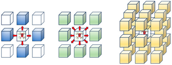
Figure 11.
The action space of UAV.
The state space s of the UAV is defined as the coordinate set of the grid where the UAV is currently located. In this model, the path-planning environment of the UAV has been gridded and expressed according to the local grid position identification system. The code of the local grid position identification system is unique in this task space. Different spatial regions correspond to different grids, and different grids are mapped to unique grid codes. In this model, the local area network location identification system codes of the UAV’s current location grid are used as the current state of the UAV, and the state space is the local area network location identification system code set for the UAV’s current grid.
The setting of the reward function R plays a certain guiding role in the pathfinding process of the UAV in this model. This study adopts the three-dimensional diagonal distance as a metric for quantifying the flight distance of the UAV. The definition of the three-dimensional diagonal distance is shown in Figure 12 as follows:
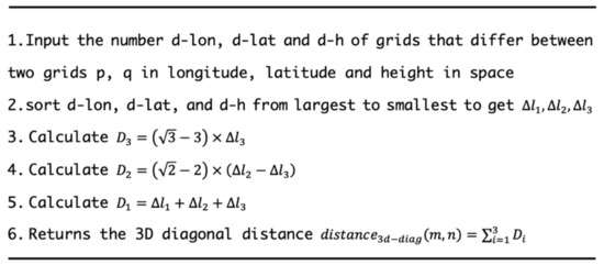
Figure 12.
The calculation of three-dimensional diagonal distance flow chart.
Define the reward function r such that it is negatively correlated with the three-dimensional diagonal distance between the current grid q and the destination grid. As shown in Formula (4) below, the smaller the three-dimensional diagonal distance from the current point to the destination, the greater the reward value.
UAV flights in urban spaces need to maintain a safe distance from obstacles to avoid collisions. Traditional algorithms, like A*, may lead UAVs too close to buildings, increasing collision risk. As urban density continues to grow, it is becoming harder for drones on low-altitude missions to maintain safe distances. Given constraints on power and mission time, UAVs need to reach destinations quickly. Thus, it is crucial for UAVs to autonomously navigate “optimal flight paths” that satisfy mission speed and safety requirements. This need for intelligent path-finding to balance efficiency and safety is increasingly critical in dynamic urban environments.
Considering the stated issues, this model sets a traffic cost for areas near obstacles. The model does not entirely preclude traversal of airspace near structures; rather, it assigns penalties to UAV actions that bring it close to obstacle surfaces [9]. Defined herein, the traffic cost around an obstacle corresponds to an open interval between 0 and 1. The traffic cost of a grid cell housing an obstacle is 1, and the cost for the airspace grid close to an obstacle is a real number between 0 and 1. Specifically, the traffic cost for the first layer grid around the obstacle is set as , while for the second layer, it is , and so on until the Nth layer grid traffic cost . The traffic cost is 0 for free-airspace grids situated further out than the safe distance boundary. The selection of this safety distance boundary is designated by the user, keeping the UAV scale and mission environment in mind. Similarly, the values are also determined through Formula (5) below set by the user:
If the UAV’s current position borders an obstacle or mission area limit and the next action dictated by the exploration strategy would result in collision or boundary transgression, this model overrides that action: the UAV stays at its original spot, maintaining its current state.
The exploration methodology adopted is the classic approach . Under this strategy, the UAV will not enter grid cells where obstacles are located, i.e., those with a passage cost of 1. Therefore, the range of the passing cost of the grid that the UAV can pass is [0, 1).
This model will learn from the ideas of Jun et al.’s paper to improve the reward mechanism and improve the reward function R, as shown in Formula (6).
In this context, refers to the traffic cost in grid n. The value of i is associated with the distance between grid n and the obstacle/mission boundary. is a positive real number and can be adjusted in the formula as a passage cost parameter. Given that , . Multiplying it by gives a value that is less than 0, so the larger the value of , the greater the traffic cost penalty inflicted on the UAV. The termination conditions for the task are either reaching the target area or exceeding the maximum number of flight steps (a user-determined value). The maximum capacity for the experience replay pool is also user-defined. If the capacity is exceeded, the initial experience quadruple will be replaced by the most recent experience quadruple entering the pool.
Neural Network Model’s Construction:
The process of constructing a neural network model begins with the specification of input and output forms. The input form is initiated by the state space of the UAV. In this model, as the UAV’s state is defined as the position code of its current location, the input is an n-bit local grid position identity code, essentially a 1-by-n vector. The output form corresponds to the action space of the UAV. Given that the UAV engages in an m-neighborhood flight mode, the output becomes a 1 × m vector, representing the Q values of m actions, respectively. Following the specification of the inputs and outputs, the neural network’s internal architecture can then be formulated. With respect to UAV path-planning tasks, a simplistic multi-layer perceptron fulfills the task of learning. This model utilizes the traditional multi-layer perceptron architecture. Its details are as follows:
Input Layer: A 1 × n vector;
Hidden Layers: Two layers—the first layer consists of 100 neurons, and the second layer encompasses 200 neurons (the number of neurons can be customized by the user);
Output Layer: A 1 × m vector.
Hence, the organization of the network is as follows:
Input Layer (1 × n) -> Hidden Layer 1 (100 neurons) -> Hidden Layer 2 (200 neurons) -> Output Layer (1 × m).
This uncomplicated, multi-layer perceptron is adequate for learning the optimal policy for UAV path planning.
3. Results
The two experiments discussed in this section were carried out using the same hardware and software environment. The key configurations are as follows:
Hardware environment:
CPU—Intel(R)Core(TM)i5-10400F CPU@2.90GHz;
GPU—NVIDIA GeForce GTX 1650, 4GB;
Memory—16 GB 2933 MHz;
Hard disk—UMIS RPJTJ256MEE1OWX, 256 GB.
Software environment:
Operating system—Windows 10 64bit;
Graphics card driver—nvldumdx.dll 30.0.14.7239 and CUDA 11.0;
Languages and Compilers—Python 3.8 and Spyder 4.1.5;
Main dependent libraries—OpenCV-Python 4.5.5.62, Matplotlib 3.3.2, Mayavi 4.7.2, Numpy 1.22.3, and Torch 1.7.1;
Map-processing software—ArcGIS 10.7 and Cesium 1.7.5.
According to the workflow of the deep-reinforcement-learning grid model, the first step for a specific application is to start from the demand layer and clarify the specific needs in the UAV path-planning process. In the mission area, the GeoSOT grid map of the mission area must first be given, and then the geographical elements in the mission area should be expressed in a grid. After these steps are completed, path planning can be carried out. The method of gridding the task area and elements within the area has been given in Part 2. In this model, the real world is abstracted, and each individual space is designated as a toll, so this method is practical.
Taking the UAV 3D scene path-planning data from the East Gate of the Peking University Remote Sensing Building as the background, there is clearly a requirement for obstacle avoidance. The starting point of this task scene is a point near the East Gate of Peking University. The selected latitude and longitude coordinates are about (116.3219° E, 39.9966° N, 0 m) and (116.3189° E, 39.9991° N, 0 m); the task area is shown in Figure 13 below.
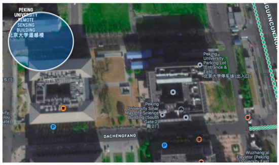
Figure 13.
The mission area.
Based on the size of the current mission area, the 23rd level grid (with a scale of approx. 8 m near the equator and 4 m near the mission area) of GeoSOT was utilized to partition the environment. Considering the UAV’s flight altitude, only the Lui Che Woo Building and Jinguang Life Science Building are taller structures in the area, so they were treated as obstacles.
The latitude/longitude coordinates of the lower right and upper left corners of the Lui Che Woo Building are approximately (116.3200° E, 39.9981° N, 0 m) and (116.3192° E, 39.9987° N, 0 m). Similarly, for the Jinguang Life Sciences Building, these coordinates are (116.3214° E, 39.9981° N, 0 m) and (116.3214° E, 39.9981° N, 0 m). The obstacle area is depicted in Figure 14.
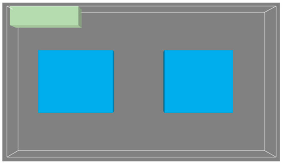
Figure 14.
The obstacle area.
From a two-dimensional perspective, in this experiment, we assigned the remote sensing building as the upper left corner of the task area, used the 23rd-level grid of GeoSOT-3D as a standard, and gridded the task area into a cuboid area. Among them, the elevations of the Remote Sensing Building, the Lui Che Woo Building, and the Jinguang Life Science Building are all five GeoSOT-3D level-23 grid side lengths. The top view of the task area after division is shown in Figure 15.
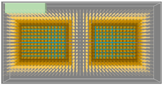
Figure 15.
The gridded task area.
The task area grid set belongs to the same parent grid at the 16th level of GeoSOT-3D. According to the local grid position identification system, this parent grid can be used as a new 0-level subdivision unit, and the grid of this area can be recoded. After encoding, the grid code length of each grid was reduced from 69 bits to 21 bits (7 bits for longitude + 7 bits for latitude + 7 bits for height).
Experiment 1 was conducted to validate the proposed GeoSOT-based deep-reinforcement-learning approach for UAV path planning in comparison to using local single-scale grid indices as inputs. The deep RL algorithm employs DQN and Nature DQN, with the UAV exploring via 4-neighborhood, 8-neighborhood, and 26-neighborhood navigation policies, and the reward function R uses Formula (4). Each experimental group was repeated 30 times, measuring the success rate of the UAV reaching the target area.
The neural network parameters were initialized randomly. The discount factor was used to measure the importance of future rewards in the current state; a larger discount factor means that the agent pays more attention to future rewards, while a smaller discount factor means that the agent pays more attention to immediate rewards. The exploration rate determines the probability of exploring new actions; a higher exploration rate helps to discover better strategies, but it may render the agent unable to converge for a long time, while a lower exploration rate may cause the agent to fall into a local optimal solution. Based on experience gained from related works [12], the following key hyperparameters (listed in Table 1) were used:

Table 1.
Experiment 1 hyperparameter setting table.
The experimental results are shown in Figure 16.
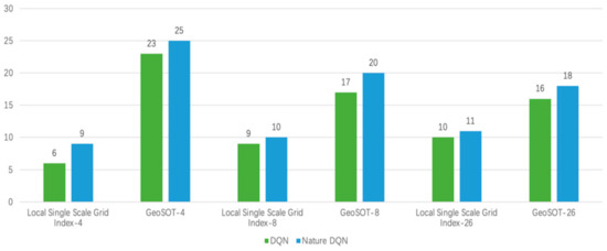
Figure 16.
Graph of the results of Experiment 1.
The task success rate data are organized as shown in Table 2 below:
Table 2.
Results comparison for Experiment 1.
The experimental results show that no matter what flying method the UAV adopts, the deep-reinforcement-learning algorithm adopts DQN or Nature DQN. The GeoSOT local grid position coding system has a greater success rate for the task success rate than the local grid index as the input of the neural network. This improvement indicates that the input method makes the algorithm more likely to converge, and its anti-interference ability is stronger, that is, the training is more stable.
Experiment 2 involved the meticulous process of assigning traffic costs for potential obstacles within the task region along with the adjoining airspace grids. In line with the aforementioned approach, the traffic cost for any grid containing a physical obstacle was set to 1, with a safe distance defined as five grid lengths (N = 5). The traffic cost of the first layer of the outsourced grid for obstacles is 5∕6 ≈ 0.83, the traffic cost of the second layer of the outsourced grid is 4∕6 ≈ 0.67, and the traffic cost of the third layer of the outsourced grid is 3∕6 = 0.50. The traffic cost of the fourth layer of the outsourced grid is 2∕6 ≈ 0.33, the traffic cost of the fifth layer of the outsourced grid is 1∕6 ≈ 0.17, and the traffic cost of the airspace grid outside the safe distance is 0.
The color depth and grid size were used to represent the size of the outsourced grid traffic cost (the darker the color and the larger the grid, the greater the traffic cost). A 3D image of the task area after the traffic cost has been set is shown in Figure 17.
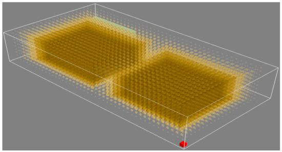
Figure 17.
A schematic diagram of the traffic cost in the experimental environment. The red block is the start point of the path.
In Experiment 2, the Nature DQN algorithm was used, employing the reward mechanism R as designated in Formula (6) for setting purposes, and the parameter initialization method of the neural network was randomly initialized. The experiment was divided four times, the deep-reinforcement-learning grid model proposed in this paper was used three times, and the adjustable parameter μ was set to 0, 0.4, and 0.5, respectively. When μ = 0, this means that the reward function does not consider the third item; that is, the UAV does not consider the traffic cost at all. When μ is 0.4 and 0.5, this means that the traffic cost is considered, and the degree of consideration is different. The fourth experiment involved the classic A* algorithm. The hyperparameter settings of the first three experiments are shown in Table 3 below.
Table 3.
Experiment 2 hyperparameter setting table.
The results of the four experiments are as follows:
The result of μ = 0 is shown in Figure 18a–d are the top views and three-dimensional views of the test results.
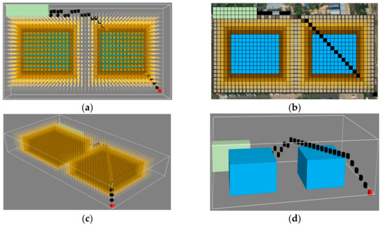
Figure 18.
Experimental results when μ = 0. (a) Top view of μ = 0 experimental results. (b) Top view of μ = 0 experimental results (created using Cesium). (c) 3D view of μ = 0 experimental results. (d) A 3D view of μ = 0 experimental results (the traffic cost is not displayed).
In the above results, it can be seen that without considering the traffic cost, some of the grids in the planned path are connected to the surfaces of obstacles, for which the number is 12, which is undoubtedly a safety hazard for UAV flight. Similarly, the results of μ = 0.4 and μ = 0.5 are also shown in the figure below. Figure 19, Figure 20 and Figure 21 represent the results of the second and third experiments, respectively.
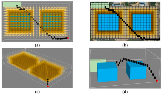
Figure 19.
μ = 0.4 experimental results. (a) Top view of μ = 0.4 experimental results. (b) Top view of μ = 0.4 experimental results (created using Cesium). (c) 3D view of μ = 0.4 experimental results. (d) A 3D view of μ = 0.4 experimental results (the traffic cost is not displayed).
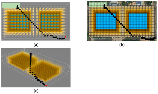
Figure 20.
μ = 0.5 experimental results. (a) Top view of μ = 0.5 experimental results. (b) Top view of μ = 0.5 experimental results (created using Cesium). (c) Three-dimensional view of μ = 0.5 experimental results.
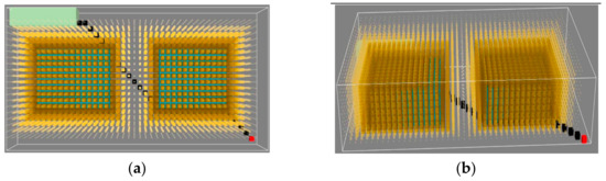
Figure 21.
The fourth set of experimental results (A*). (a) Top view of A* experimental results. (b) Three-dimensional view of A* experimental results.
According to the above results, when μ = 0.4 is adjusted, the UAV has already begun to consider the impact of the traffic cost when planning the path and no longer flies close to the surface of an obstacle, which effectively increases the safety of the UAV’s flight process. When adjusting μ = 0.5, the UAV chooses a grid flight with a higher altitude and lower traffic cost, which more effectively increases the safety of the UAV’s flight.
The results of Experiment 4 show that the A* algorithm makes the UAV choose to fly close to the ground, and a considerable part of the grid is adjacent to obstacles, which is also a safety hazard for UAV flight.
For the calculation of the path length, the side length of a single grid is, the length of flying in a straight direction corresponds to , the length of flying along a grid in a diagonal direction corresponds to , and the length along the diagonal section of a body is . The length of flying along a grid is as shown in Figure 22 below.
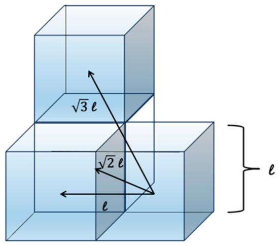
Figure 22.
Path length.
The experimental results are shown in Table 4 below.
Table 4.
Results comparison for Experiment 2.
4. Discussion
Experiment 1 indicated that the GeoSOT local grid location encoding system achieved a higher success rate for task completion compared to when local grid indexes were used as neural network inputs. The reason for this result is that the process of establishing the local single-scale grid system involved greater randomness, and the relationships between local grid indexes were not strong enough to effectively characterize the UAV’s state. This lack of valid “contextual” relationships between UAVs limited what the neural network could learn each round. In contrast, the process of establishing the local grid location identification system was non-random, with grid-to-grid relationships following a spatiotemporal z-curve filling pattern. This enabled the encoding of spatial locations as representations with richer “contextual” information. This prior structure enables more efficient learning in the complex path-planning task compared to the use of local grid indices alone.
Experiment 2 provides valuable insights into the performance of the proposed deep-reinforcement-learning grid model. When the traffic cost is not considered (μ = 0), the Nature DQN algorithm plans some UAV flight paths adjacent to building surfaces, posing safety risks. By adjusting μ to 0.4, the UAV chooses higher-altitude grids, effectively avoiding proximity to buildings. At μ = 0.5, the path-planning safety is further enhanced. As a result of the A* algorithm, the UAV chooses to fly close to obstacles and the ground, and a considerable part of the grid is adjacent to obstacles, which is also a serious safety hazard. The deep-reinforcement-learning grid model proposed in this paper performs better than A* in terms of safety for the demand improvement method considering the traffic cost. When μ = 0.5, the total path traffic cost of the planned flight path was reduced by 61.71% compared with the A* algorithm and did not exist in the grid adjacent to the building. At the same time, the experimental results show that the degree of consideration of the UAV’s flight with respect to the traffic cost can be adjusted by adjusting μ; that is, the two factors of the flight distance and safety of the UAV can be controlled degrees of importance. At the same time, the first three sets of experimental results of Experiment 2 show that adjusting μ can regulate the degree to which the drone considers the traffic cost; the larger the value of μ, the greater the impact of the traffic cost on the drone’s path planning, and the more likely it is the drone will choose a grid with a low traffic cost.
The deep-reinforcement-learning grid model put forth in this research is well suited to the increasing intelligentization of UAV path planning in the big data era. By leveraging grid encodings, it can effectively represent fundamental environmental data traits. Further integration with deep RL produced a comprehensive depiction of spatialized information like surroundings and route outputs. This grid-based DRL approach has significant foreseeable potential for civilian use cases, such as deliveries and aerial photography. It could furnish UAVs with an intelligent obstacle avoidance technique that efficiently structures environmental data while accounting for diverse influencing factors.
Concurrently, when experimenting with and applying this method, the relevant requirements of the Civil Aviation Administration of China’s “Interim Measures for the Administration of Commercial Operation of Civil Unmanned Aerial Vehicle” should be followed to ensure flight safety and prevent accidents. Specifically, in this study, the research team obtained the proper registrations and approvals as mandated, and flights were conducted according to the rules and ethical standards for unmanned aerial systems. Ensuring compliance with civil aviation regulations and operating unmanned aerial vehicles responsibly are essential for advancing scientific understanding while protecting public safety.
Looking ahead, this model can enable drones to make better contextual decisions and fly along safer trajectories. By organizing spatial knowledge and optimizing policies through experience, the deep RL grid paradigm promises the continued advancement of intelligent UAV navigation amidst complex real-world settings. Its strengths in fusing environmental encodings with adaptive learning make it an impactful contribution towards the future of AI-enabled flight planning systems.
5. Conclusions
This research makes effective use of the advancements in artificial intelligence and big data to tackle new complexities in UAV path planning. Recognizing the growing interdependence between UAV trajectory optimization and AI, this paper underscores their combined development.
The designed deep-reinforcement-learning grid model can fully express the basic characteristics of environmental data information through grids and is coupled with a deep reinforcement learning model to provide a comprehensive presentation of various types of information, such as environmental situations and path results under a spatial distribution.
Grounded in related challenges, a unified deep reinforcement learning model has been proposed within a GeoSOT global spatial framework tailored for UAVs. This novel integration harnesses GeoSOT’s capabilities in unified spatial data organization and expression along with the end-to-end solution proficiencies of deep RL.
The resulting paradigm constitutes a new approach to UAV path planning, which has been validated through scene implementations. GeoSOT’s spatial knowledge representation and deep RL’s learning capacities prove highly complementary. This harmony allows the model to address associated obstacles in the planning process. This paper provides a new investigation of the combined application of a deep-reinforcement-learning model for UAV path planning and the global subdivision grid coding system, in which some existing problems are solved or alleviated, but there are still some aspects worth exploring, such as the generalizability of deep reinforcement learning models. This paper defines the state of an unmanned aerial vehicle (UAV) as the spatial encoding of its location, which lacks generalizability. Subsequent research should consider including some property characterizations of a UAV’s neighboring grids in a given state, such as passability, enabling the neural network to learn the spatial features of the UAV’s current spatial location and neighboring properties. Through massive data training, deep-reinforcement-learning models may gain generalizability. In new, unknown environments, good predictive performance can be achieved by observing a UAV’s spatial location and neighboring features.
The deep-reinforcement-learning (DRL) grid model put forth in this research is well suited to the increasing intelligentization of UAV path planning in the big data era. By leveraging grid encodings, it can effectively represent fundamental environmental data traits. Further integration with deep RL produced a comprehensive depiction of spatialized information like surroundings and route outputs.
Overall, by leveraging AI innovations and a multi-faceted spatial framework, this research enables sophisticated UAV navigation. It lays the groundwork for continued advancement at the intersection of intelligent systems and robotics. The proposed model delivers robust and generalizable solutions, unlocking the potential of AI-empowered UAV path planning in the big data era.
It is foreseeable that the proposed deep-reinforcement-learning grid model will have the following application scenarios in the future. The first is civilian scenarios, such as express delivery, aerial photography, etc., in which the proposed model can provide UAVs with an intelligent obstacle avoidance method that can efficiently organize environmental data and consider the influence of many factors in an environment; the second is military scenarios, such as rescue in disaster areas, the selection of strike targets, etc., in which the proposed model can provide UAVs with path planning in rapidly changing complex scenes. Of course, this model still needs to be tested further in various conditions, and the criterion of wind direction and strength must be taken into account, both of which are worth exploring in future research.
Looking ahead, this model can enable drones to make better contextual decisions and fly along safer trajectories. By organizing spatial knowledge and optimizing policies through experience, the deep RL grid paradigm promises the continued advancement of intelligent UAV navigation amidst complex real-world settings. Its strengths in fusing environmental encodings with adaptive learning make the proposed model an impactful contribution towards the future of AI-enabled flight planning systems.
Author Contributions
Conceptualization, Guoyi Sun, Qian Xu and Chengqi Cheng; Data processing, Guoyi Sun and Qian Xu; Funding acquisition, Chengqi Cheng; Normalized analysis, Guoyi Sun and Guangyuan Zhang; Investigation, Guoyi Sun and Qian Xu; Project administration, Guoyi Sun, Qian Xu and Guangyuan Zhang; Methodology, Guoyi Sun and Qian Xu; Resources, Tengteng Qu; Software, Qian Xu; Supervision, Chengqi Cheng and Haojiang Deng; Validation, Guoyi Sun and Qian Xu; Visualization, Guoyi Sun and Qian Xu; Writing—original draft, Guoyi Sun; Writing—review and editing, Guoyi Sun. All authors have read and agreed to the published version of the manuscript.
Funding
This work was supported by the National Key Research and Deployment Program of China (Grant No.2020YFB1806402).
Data Availability Statement
The data is unavailable due to privacy or ethical restrictions.
Conflicts of Interest
The authors declare no conflict of interest.
References
- Fahlstrom, P.G.; Gleason, T.J.; Sadraey, M.H. Introduction to UAV Systems; John Wiley & Sons: Hoboken, NJ, USA, 2022. [Google Scholar]
- Yang, L.; Qi, J.; Xiao, J.; Yong, X. A literature review of UAV 3D path planning. In Proceedings of the 11th World Congress on Intelligent Control and Automation, Shenyang, China, 29 June–4 July 2014; IEEE: New York, NY, USA, 2014; pp. 2376–2381. [Google Scholar]
- Swinney, C.J.; Woods, J.C. A review of security incidents and defence techniques relating to the malicious use of small unmanned aerial systems. IEEE Aerosp. Electron. Syst. Mag. 2022, 37, 14–28. [Google Scholar] [CrossRef]
- Bauranov, A.; Rakas, J. Designing airspace for urban air mobility: A review of concepts and approaches. Prog. Aerosp. Sci. 2021, 125, 100726. [Google Scholar] [CrossRef]
- Ritchie, M.; Fioranelli, F.; Griffiths, H.; Torvik, B. Micro-drone RCS analysis. In Proceedings of the 2015 IEEE Radar Conference, Arlington, VA, USA, 27–30 October 2015; IEEE: New York, NY, USA, 2015; pp. 452–456. [Google Scholar]
- Lipovský, P.; Novotňák, J.; Blažek, J. Possible Utilization of Low Frequency Magnetic Fields in Short Range Multirotor UAV Detection System. Transp. Res. Procedia 2022, 65, 106–115. [Google Scholar] [CrossRef]
- Faul, F.T.; Korthauer, D.; Eibert, T.F. Impact of rotor blade rotation of UAVs on electromagnetic field measurements. IEEE Trans. Instrum. Meas. 2021, 70, 3109354. [Google Scholar] [CrossRef]
- Zhang, J.; Hu, C.; Chadha, R.G.; Singh, S. Maximum likelihood path planning for fast aerial maneuvers and collision avoidance. In Proceedings of the 2019 IEEE/RSJ International Conference on Intelligent Robots and Systems (IROS), Macau, China, 3–8 November 2019; IEEE: New York, NY, USA, 2019; pp. 2805–2812. [Google Scholar]
- Jun, M.; D’Andrea, R. Path planning for unmanned aerial vehicles in uncertain and adversarial environments. In Cooperative Control: Models, Applications and Algorithms; Springer: Berlin/Heidelberg, Germany, 2003; pp. 95–110. [Google Scholar]
- Zhang, W.; Zhang, S.; Wu, F.; Wang, Y. Path planning of UAV based on improved adaptive grey wolf optimization algorithm. IEEE Access 2021, 9, 89400–89411. [Google Scholar] [CrossRef]
- Greenwood, W.W.; Lynch, J.P.; Zekkos, D. Applications of UAVs in civil infrastructure. J. Infrastruct. Syst. 2019, 25, 04019002. [Google Scholar] [CrossRef]
- Panov, A.I.; Yakovlev, K.S.; Suvorov, R. Grid path planning with deep reinforcement learning: Preliminary results. Procedia Comput. Sci. 2018, 123, 347–353. [Google Scholar] [CrossRef]
- Yang, R.; Cheng, L. Path planning of restaurant service robot based on a-star algorithms with updated weights. In Proceedings of the 2019 12th International Symposium on Computational Intelligence and Design (ISCID), Hangzhou, China, 14–15 December 2019; IEEE: New York, NY, USA, 2019; pp. 292–295. [Google Scholar]
- Lee, J.; Huang, R.; Vaughn, A.; Xiao, X. Strategies of path-planning for a UAV to track a ground vehicle. In Proceedings of the 2nd Annual Autonomous Intelligent Networks and Systems Conference, Menlo Park, CA, USA, 14–18 July 2003. [Google Scholar]
- Koay, T.-B.; Chitre, M. Energy-efficient path planning for fully propelled AUVs in congested coastal waters. In Proceedings of the 2013 MTS/IEEE OCEANS-Bergen, Bergen, Norway, 10–13 June 2013; IEEE: New York, NY, USA, 2013; pp. 1–9. [Google Scholar]
- Reibel, M. Geographic information systems and spatial data processing in demography: A review. Popul. Res. Policy Rev. 2007, 26, 601–618. [Google Scholar] [CrossRef]
- Qian, C.; Yi, C.; Cheng, C.; Pu, G.; Wei, X.; Zhang, H. Geosot-based spatiotemporal index of massive trajectory data. ISPRS Int. J. Geo-Inf. 2019, 8, 284. [Google Scholar] [CrossRef]
- Li, D.; Jiang, J.; Jiang, C. Multi-agent reinforcement learning flight path planning algorithm. Electron.-Opt. Control 2009, 16, 10–14. [Google Scholar]
- Mnih, V.; Kavukcuoglu, K.; Silver, D.; Graves, A.; Antonoglou, L.; Wierstra, D.; Riedmiller, M. Playing atari with deep reinforcement learning. arXiv 2013, arXiv:1312.5602. [Google Scholar]
- Mnih, V.; Kavukcuoglu, K.; Silver, D.; Rusu, A.A.; Veness, J.; Bellemare, M.G.; Graves, A.; Riedmiller, M.; Fidjeland, A.K.; Ostrovski, G.; et al. Human-level control through deep reinforcement learning. Nature 2015, 518, 529–533. [Google Scholar] [CrossRef]
- Rovel, L.; Wei, R.; Ding, C. Intelligent UAV path planning method based on deep reinforcement learning DQN. In Proceedings of the 2019 Chinese Automation Congress (CAC 2019), Hangzhou, China, 22–24 November 2019. [Google Scholar]
- Shorakaei, H.; Vahdani, M.; Imani, B.; Gholami, A. Optimal cooperative path planning of unmanned aerial vehicles by a parallel genetic algorithm. Robotica 2016, 34, 823–836. [Google Scholar] [CrossRef]
- Hu, X.; Cheng, C. The three-dimensional data organization method based on GeoSOT-3D. In Proceedings of the 2014 22nd International Conference on Geoinformatics, Kaohsiung, Taiwan, 25–27 June 2014; IEEE: New York, NY, USA, 2014; pp. 1–4. [Google Scholar]
- Xiaoguang, H.U.; Chengqi, C.; Xiaochong, T. The Representation of Three-Dimensional Data Based on GeoSOT-3D. Acta Sci. Nat. Univ. Pekin. 2015, 51, 1022. [Google Scholar]
- Zhai, W.; Qi, C.; Cheng, C.; Li, S. Spatial data management method with GeoSOT grid. In Proceedings of the 2017 IEEE International Geoscience and Remote Sensing Symposium (IGARSS), Fort Worth, TX, USA, 23–28 July 2017; IEEE: New York, NY, USA, 2017; pp. 5217–5220. [Google Scholar]
- Han, B.; Qu, T.; Tong, X.; Jiang, J.; Zlatanova, S.; Wang, H.; Cheng, C. Grid-optimized UAV indoor path planning algorithms in a complex environment. Int. J. Appl. Earth Obs. Geoinf. 2022, 111, 102857. [Google Scholar] [CrossRef]
- Zhai, W.; Han, B.; Li, D.; Duan, J.; Cheng, C. A low-altitude public air route network for UAV management constructed by global subdivision grids. PLoS ONE 2021, 16, e0249680. [Google Scholar] [CrossRef] [PubMed]
- Qi, K.; Cheng, C.; Hu, Y.; Fang, H.; Ji, Y.; Chen, B. An improved identification code for city components based on discrete global grid system. ISPRS Int. J. Geo-Inf. 2017, 6, 381. [Google Scholar] [CrossRef]
Disclaimer/Publisher’s Note: The statements, opinions and data contained in all publications are solely those of the individual author(s) and contributor(s) and not of MDPI and/or the editor(s). MDPI and/or the editor(s) disclaim responsibility for any injury to people or property resulting from any ideas, methods, instructions or products referred to in the content. |
© 2023 by the authors. Licensee MDPI, Basel, Switzerland. This article is an open access article distributed under the terms and conditions of the Creative Commons Attribution (CC BY) license (https://creativecommons.org/licenses/by/4.0/).