Discovering Spatio-Temporal Co-Occurrence Patterns of Crimes with Uncertain Occurrence Time

Abstract

The discovery of spatio-temporal co-occurrence patterns (STCPs) among multiple types of crimes whose events frequently co-occur in neighboring space and time is crucial to the joint prevention of crimes. However, the crime event occurrence time is often uncertain due to a lack of witnesses. This occurrence time uncertainty further results in the uncertainty of the spatio-temporal neighborhood relationships and STCPs. Existing methods have mostly modeled the uncertainty of events under the independent and identically distributed assumption and utilized one-sided distance information to measure the distance between uncertain events. As a result, STCPs detected from a dataset with occurrence time uncertainty (USTCPs) are likely to be erroneously assessed. Therefore, this paper proposes a probabilistic-distance-based USTCP discovery method. First, the temporal probability density functions of crime events with uncertain occurrence times are estimated by considering the temporal dependence. Second, the spatio-temporal neighborhood relationships are constructed based on the spatial Euclidean distance and the proposed temporal probabilistic distance. Finally, the prevalent USTCPs are identified. Experimental comparisons performed on twelve types of crimes from X City Public Security Bureau in China demonstrate that the proposed method can more objectively express the occurrence time of crimes and more reliably identify USTCPs.

1. Introduction

Crimes are a major issue in modern society. To take effective measures to reduce crime, it is crucial to deeply understand its occurrence mechanisms. Currently, most studies attempt to explore the relationship between crime occurrence and the physical environment [1,2]. These studies are primarily aimed at facilitating the prevention of a single type of crime. In criminology, the boost theory suggests that crimes exhibit spatio-temporal interaction [3]. Under this theory, different types of crimes may occur together in spatio-temporal neighborhoods. Such patterns are identified as spatio-temporal co-occurrence patterns (STCPs) [4]. Discovering the STCPs of crimes can reveal the spatio-temporal associations underlying the occurrence of different types of crimes, which can help the police develop effective joint prevention and control measures for multiple types of crimes to reduce economic loss and guarantee public safety.

Police crime records detail the victim’s personal information, crime type, and address and time of crime occurrence. With the development of geocoding technologies, crime locations can be mapped with a considerable degree of precision [5]. However, it is difficult for the victims and police to obtain the exact occurrence time of some crime events due to a lack of witnesses [6]. The occurrence time of a crime event is often recorded as an interval, i.e., [start time, end time], which indicates the range of possible times that the crime event could have occurred. For instance, say that someone left home at 10:00 a.m. on 1 January 2022 and found that something had been stolen when they returned home at 2:00 p.m. on the same day. Then, the occurrence time of this burglary event is recorded as [1 January 2022 10:00, 1 January 2022 14:00]. The occurrence time uncertainty of crime events will cause uncertainty in the spatio-temporal neighborhood relationship between crime events and further cause the STCPs to be uncertain. In this study, the STCPs detected from a spatio-temporal dataset with occurrence time uncertainty are referred to as uncertain STCPs (USTCPs).

Recent studies have developed two types of methods to mine USTCPs: the expected-distance-based and the possible-world-based methods. The former first utilizes probability distribution functions to independently model the uncertainty of the possible occurrence locations for each event. The expected distance is then defined (i.e., the expected value of possible Euclidean distances between uncertain events) to describe the spatio-temporal neighborhood relationship. Finally, the prevalence of candidate USTCPs can be measured, as in a deterministic dataset [7]. The latter models an uncertain dataset as a set of deterministic datasets, i.e., possible worlds, by combining the discrete possible occurrence locations of events. The existential probability of each possible world is the product of the occurrence probabilities of the events in it. The prevalence of a candidate USTCP is evaluated by integrating the existential probability and the frequency with which all included features (i.e., categories) occur together in each possible world [8,9]. Previous studies have modeled uncertain datasets assuming that geographic events are mutually independent, which is contrary to the fact that geographic observations are spatially and temporally dependent [10,11]. Additionally, the numerical distance, i.e., a distance value aggregating the part of the possible distances between uncertain events, cannot reflect the full spatio-temporal relationship. The inherent limitations of existing methods make the reliability of the detected USTCPs questionable. Therefore, this paper proposes a probabilistic-distance-based approach to discover USTCPs among crimes with uncertain occurrence times. This method first characterizes the temporal probability distribution of crime event occurrence using a kernel density estimation function that considers the dependence among events. Based on this, we adopt a probabilistic distance to accurately describe the spatio-temporal relationship between events. In this manner, USTCPs with high prevalence are discovered. The proposed method is expected to more reliably discover the USTCPs among multiple crimes with uncertain occurrence times. To verify this, an empirical study on the crime dataset in X city, China, is conducted.

The remainder of this paper is organized as follows. Section 2 reviews and critically analyzes the related work on uncertain co-occurrence pattern discovery. Section 3 presents the proposed approach for detecting USTCPs based on probabilistic distance. In Section 4, the results of the USTCPs are analyzed using a real urban crime dataset. Finally, the conclusions and future work are provided in Section 5.

2. Related Work

Co-occurrence patterns refer to subsets of features (i.e., categories) whose events frequently occur together and can be divided into three categories according to the type of target dataset: association rules discovered from transaction datasets [12], spatial co-occurrence patterns discovered from spatial datasets [13,14], and STCPs discovered from spatio-temporal datasets [15]. In recent years, extensive studies have been conducted on deterministic and uncertain datasets. Herein, the co-occurrence patterns detected in uncertain datasets are referred to as uncertain co-occurrence patterns. Unlike near-repeat patterns [3] and spatio-temporal hotspot patterns [16], which identify the correlation between crime events with a single type (i.e., auto-correlation), co-occurrence patterns can reveal additional knowledge regarding the associations among different types of crime events (i.e., cross-correlation).

The process for discovering co-occurrence patterns in a deterministic dataset mainly consists of two steps. First, the co-occurrence instances (i.e., pairs of events) satisfying the neighborhood relationship for each candidate co-occurrence pattern are identified. Second, the prevalence of the candidate co-occurrence patterns (i.e., the frequency of different features co-occurring) is measured, and patterns with sufficiently high prevalence are detected. For the transaction dataset, events in the same transaction are considered neighbors, and then, support and confidence are defined to measure the prevalence of association rules [12]. To overcome the limitation that there is no natural notion of transactions in geographic space, a transaction-based model is developed for detecting spatial co-occurrence patterns. This model constructs spatial transactions via space partitioning [17], which often loses the spatial neighborhood relationship at the transaction boundary. Therefore, a transaction-free model is further proposed [13,18]. This model identifies a group of events as a co-occurrence instance if the spatial distance between them is less than a specified distance threshold. The prevalence of each candidate spatial co-occurrence pattern is evaluated using a participation index (i.e., the minimum participation ratio of the included features). The participation ratio of a feature is the ratio of the number of events in a feature that satisfy the neighborhood relationship with events of other features in that pattern to the total number of that feature’s events in the dataset. By integrating the time dimension in the transaction-free model, two types of methods are developed to discover STCPs: the divide-and-conquer method and the coupling method. The former first divides spatio-temporal events into different time slots via time partitioning and then executes a spatial co-occurrence pattern mining algorithm in each time slot. The spatial co-occurrence patterns that frequently occur in several time slots are identified as STCPs [19,20]. However, the time dimension partitioning scheme is likely to break up the temporal neighborhood relationship between events in adjacent time slots [21]. The latter method handles the time dimension as an alternative spatial dimension and constructs the spatio-temporal neighborhood relationship among events based on spatial and temporal distances. Furthermore, the subsets of features whose events frequently co-occur in spatial and temporal neighborhoods are identified as STCPs [22,23].

Regarding uncertain datasets, existing studies have focused on discovering co-occurrence patterns from uncertain datasets with two types of uncertainties: existential uncertainty and attribute-level uncertainty [24]. If it is unknown whether an event is present in or absent from a transaction or location, it is considered to have existential uncertainty. If the location of an event is imprecise, we can consider that the event has an attribute-level uncertainty. Following the process of discovering co-occurrence patterns in a deterministic dataset, two types of methods are proposed to discover uncertain co-occurrence patterns: the expected-distance-based and the possible-world-based methods. These are reviewed in detail below.

2.1. Discovery of Uncertain Co-Occurrence Patterns Based on the Expected Distance

The expected-distance-based methods are generally used to mine uncertain co-occurrence patterns from a spatial dataset containing attribute-level uncertainty. First, each uncertain geographic event is assigned a probability distribution function, representing the probability that the event appears in a possible location. The occurrence probability of an event is described by a probability mass function in the discrete domain and as a probability density function in the continuous domain. Subsequently, an expected distance function is exploited to measure the spatial distance between pairs of events. Specifically, for a deterministic event and an uncertain event, mathematically, the expected distance is an integral involving the Euclidean distance between two events and the probability distribution function [25]. For two uncertain events, the respective center point (i.e., the mean) can be acquired from the probability distribution function. Then, two expected distances can be obtained by separately calculating the determined center point and another uncertain event. The spatial distance of the two uncertain events is defined as the maximum value of the two obtained asymmetric expected distance values [26]. The expected-distance-based methods identify the co-occurrence instances of candidate patterns based on the numerical distance. Then, the participation index defined in the deterministic dataset is used to evaluate the prevalence of the uncertain co-occurrence patterns [7].

Most studies often used the predefined probability distribution function to independently characterize the probability distribution function for each uncertain event. For example, Ngai et al. first generated a series of random values representing the probability mass values for all possible positions of each uncertain spatial event and then normalized the value based on the fact that the sum of the occurrence probabilities in all possible positions is one [27]. Lu et al. utilized the normal distribution function to describe the uncertainty of each uncertain event’s location in the spatial continuous domain [7]. In addition, other common probability density functions, such as the uniform and binomial distribution functions, are also used to model the occurrence location uncertainty [28].

Such strategies can also be applied to handle the occurrence time uncertainty of crime. Intuitively, the occurrence probability over the time interval of each event is described as an elementary probability distribution function. Alternatively, for each crime event, finite time stamps can be constructed by dividing the occurrence time interval and generating a probability mass value for each discrete point. Related research has shown that the expected distance is sensitive to the form and parameters of the probability distribution function [28]. However, in practice, it is difficult to determine suitable functional forms and parameters without sufficient prior knowledge.

2.2. Discovery of Uncertain Co-Occurrence Patterns Based on the Possible World

The possible-world-based methods can be used to handle both existential and attribute-level uncertainties and to mine uncertain co-occurrence patterns in transaction and spatial datasets. Regarding an uncertain dataset containing existential uncertainty, each event has two possible discrete states: existence or non-existence. Each state is associated with a probability. Possible-world-based methods first model the uncertain dataset as several deterministic datasets. Each deterministic dataset is called a possible world, which is a combination of the possible state of each event in the dataset. The existential probability of a possible world is calculated under the assumption that events are independent and is expressed as the product of the state probabilities of the events in it [29]. For each possible world, the deterministic mining methods can be reused to evaluate the prevalence of candidate co-occurrence patterns. On this basis, existing studies have proposed two indexes to measure the prevalence of uncertain co-occurrence patterns: expected prevalence and probabilistic prevalence. The uncertain co-occurrence patterns are considered valid when the expected or probabilistic prevalence is greater than a predefined threshold. The expected prevalence is essentially a weighted prevalence, which is the accumulation of the product of each possible world’s existential probability and the candidate pattern’s prevalence [30]. To reveal more information about uncertain co-occurrence patterns, the prevalence of patterns is further defined in a probabilistic manner [8]. The probabilistic prevalence is the sum of the existential probabilities of the possible worlds where the candidate pattern is prevalent [31].

Compared with studies involving existential uncertainty, the state set of each spatial event containing attribute-level uncertainty is the discrete locations where it may appear. In addition, a new interest measure is proposed to assess the prevalence of uncertain co-occurrence patterns. Specifically, for each possible world, the participation ratio of different features included in the candidate pattern is first calculated. Subsequently, the expected participation ratio of each feature is calculated, which is expressed as the accumulation of the product of the possible world’s existential probability and the corresponding participation ratio. Finally, the minimum expected participation ratio of all features in that pattern is defined as the participation index to evaluate the prevalence of patterns [9]. Possible-world-based methods have also been applied in the field of criminology to address the uncertainty of the occurrence time of crimes. For example, several studies simply adopted a single value in the occurrence time interval, such as the start time, end time, average time, or randomly taken time, to model a single possible world of the crime dataset [32,33]. To more accurately estimate the occurrence time of crimes, four extension methods have been developed [33]: aoristic, aoristic_ext, retrospective temporal approximation, and extended retrospective temporal approximation methods. These methods assign a probability value to each possible world represented by a time slot in which a crime event may occur.

2.3. Critical Analysis of Existing Studies

The occurrence time uncertainty of crime in this study is attributed to attribute-level uncertainty. The two types of existing methods can be migrated to handle the occurrence time uncertainty and detect the USTCPs of crimes. However, through a full review of relevant studies, we found that the existing studies have the following limitations.

(i) The existing methods mostly ignore the spatial and temporal dependence of geographic observations in modeling attribute-level uncertainty. As a result, the uncertainties of events cannot be objectively interpreted. For example, the dataset displayed in Figure 1 contains two types of crimes. The expected-distance-based methods may use a uniform distribution function to describe the uncertainty of each event’s occurrence time. In this manner, the probability of any event, such as B.1 or B.2, occurring at any timestamp in the corresponding time interval [start time, end time] is uniform. However, considering the temporal dependence between the events of crime B, the temporal probability distributions of events B.1 and B.2 are different. B.1 and B.2 have a greater occurrence probability around the start and end times, respectively, compared with other possible locations. Additionally, because events in different transactions are mutually independent, for the problem of discovering uncertain co-occurrence patterns from an uncertain transaction dataset, the possible-world-based methods can express the existential probability of possible worlds in the form of probability multiplication and can perform well [29,34]. However, in terms of uncertain spatio-temporal datasets, the existential probability of possible worlds may deviate greatly from the actual probability by neglecting the dependencies [35].

(ii) The currently used methods construct the spatio-temporal neighborhood relationship based on the numerical distance, which loses a large amount of distance information between uncertain events and likely makes the proximity relationship biased [36]. For the expected-distance-based methods, the expected distance is a smooth value that aggregates the possible distances relative to the center point. Taking Figure 1 as an example, events A.1 and B.3 separately occur in the time intervals [1, 5] and [2, 3]. Assuming that the occurrence probability of two events follows a uniform distribution in time, then the probability density function of these two events can be expressed as ${pdf}_{A.1}\left(t\right) = \frac{1}{4}$ (t∈[1, 5]) and ${pdf}_{B.3}\left(t\right) = 1$ (t∈[2, 3]), where t is the time dimension of the events. The center points are 3 and 5/2, respectively. The temporal expected distance between the center points of A.1 and B.3 is ${\int }_2^3{pdf}_{B.3}\left(t\right)\left|3-t\right|dt=1/2$, and the temporal expected distance between the center points of B.3 and A.1 is ${\int }_1^5{pdf}_{A.1}\left(t\right)|\frac{5}{2}-t|dt=17/16$. The temporal distance between A.1 and B.3 is the maximum value of the two asymmetric expected distance values, i.e., 17/16. These two events are not neighborhoods when the temporal distance threshold is one. In fact, the probability that the temporal distance between them is less than one is evidently high. For the possible-world-based methods, most studies use a single value in the time interval to model the crime dataset as a unique possible world [32]. Then, the USTCPs can be mined following the operations on a deterministic dataset. However, the temporal neighborhood relationship and the USTCPs identified using partial information will result in difficult decision making in practice. For example, Figure 2 exhibits two possible worlds of the uncertain dataset in Figure 1 under different occurrence time expressions. Clearly, the results obtained from the two possible worlds are conflicting: crimes A and B frequently occur together under the start time expression (Figure 2a) but not under the end time expression (Figure 2b).

To discover reliable USTCPs, it is necessary to appropriately express uncertain datasets and accurately identify the spatio-temporal proximity relationships between events. For this purpose, this study proposes a probabilistic-distance-based method to discover the USTCPs of crimes with uncertain occurrence times. First, the temporal dependence of crime events is considered to estimate the temporal probability density function of each event. Second, the geometric distance in space and the probabilistic distance in time between different types of crime events are measured, and the spatio-temporal neighborhood relationships are identified. Based on this, highly prevalent USTCPs are determined. The following section introduces the three parts in detail.

3. Methodology

3.1. Modeling the Temporal Probability Density Function of Crime Events

Establishing an appropriate expression model for an uncertain dataset is a prerequisite for a convincing construction of spatio-temporal neighborhood relationships. In criminology, the near-repeat phenomenon suggests that crime events are temporally dependent [34]. The occurrence time dependence makes the temporal occurrence probability distribution of crime events too complicated to be characterized by a predefined probability distribution function under the independent and identically distributed assumption. The kernel density estimation method can consider the dependence among observation events and can nonparametrically estimate the local point intensity [37]. Thus, this study employs the kernel density estimation method to estimate the occurrence time probability density function for each crime event.

For a type of crime containing n events, C_k = {e₁, e₂, …, e_i, …, e_n}, e_i is a crime event denoted as e_i = {(sx_i, sy_i), [t_{i_start}, t_{i_end}]}, where (sx_i, sy_i) is a tuple of spatial coordinates, and t_{i_start} and t_{i_end} are the boundaries of the time interval in which e_i may occur. Functional facilities and human activities have been demonstrated to be critical driving forces for triggering the occurrence of crime events [38]. The driving factors that repeatedly operate on a daily basis further allow crime to occur cyclically at the day level [39]. For example, in an entire day, robbery has a high incidence between 20:00 and 00:00 [40]. Therefore, the probability of a crime event occurring at a possible local timestamp can be estimated by considering the temporal dependence in a day unit.

First, given a temporal analysis scale r, in a day unit, all possible occurrence timestamps of n events belonging to crime C_k in the different time intervals are extracted and denoted as POT_k. Based on this, the temporal population distribution of crime C_k in a day unit is estimated using the kernel density estimation method:

$$f_k\left(q\right)=\frac{1}{{Nh}_k}{\displaystyle \sum }_{p\in {POT}_k}\frac{1}{\sqrt{2\pi }}{e}^{-{\left(\frac{q-p}{\sqrt{2}{h}_k}\right)}^2}, q\in (0, 24]$$

(1)

where f_k(q) represents the probability of a C_k event appearing at timestamp q, N is the number of timestamps of POT_k, and the Gaussian kernel function is selected to quantify the temporal dependence of timestamp p on q. Following the suggestion of Silverman [41], the kernel bandwidth h_k is set as 1.06 × δ_k × N^(−1/5), where δ_k is the standard deviation of possible occurrence timestamps in POT_k. For crime C_k, each event e_i is a sample of that type of crime, such that the temporal probability distribution of e_i also follows the population distribution. The temporal probability density function of e_i can then be generated as follows:

$${pdf}_i{\left(t\right)=w}_i{f}_k\left(day\right(t\left)\right), t\in {[t}_{i\_start}{, t}_{i\_end}]$$

(2)

where day(·) is a function to obtain the time information of timestamp t in a day unit, and w_i is the adjustment coefficient to satisfy the well-known property of the probability density function; that is, the integral over the domain is one. The parameter w_i is expressed as

$$w_i=1/{{\displaystyle \int }}_{t_{i\_start}}^{t_{i\_end}}{f}_k\left(day\right(t\left)\right)dt$$

(3)

As an example, for a type of crime C_k containing the three events exhibited in Figure 3a, POT_k with r = 0.5 h is obtained, and the frequency of the different timestamps in it is displayed in Figure 3b. The temporal population distribution of C_k in a day unit calculated using formula (1) is shown in Figure 3c. Evidently, crime C_k has a high probability of occurring from 6:00–8:00. Figure 3d shows the temporal probability density functions of the three events in the respective time intervals.

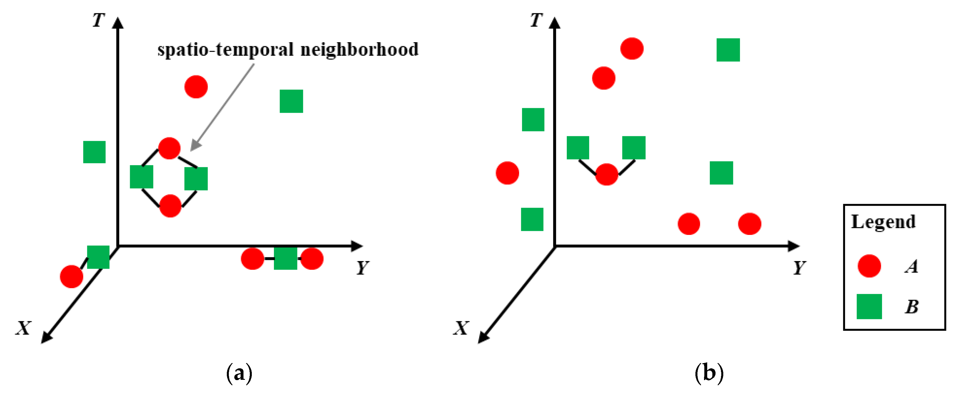
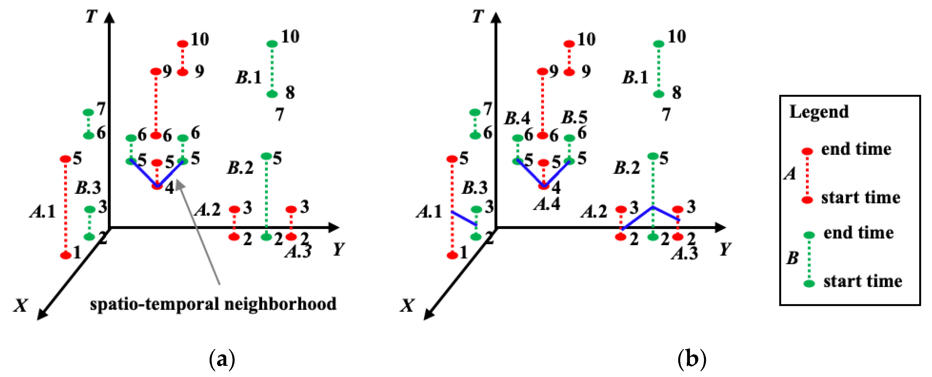
3.2. Constructing the Spatio-Temporal Neighborhood Relationship among Crime Events

As analyzed in Section 2.3, the existing numerical distance measures are aggregations of the partial possible distances between uncertain events, resulting in a biased identification of spatio-temporal neighborhood relationships. To avoid the loss of information about the distance between events, we employ probabilistic distance to describe the temporal relationship between crime events [42]. Specifically, the probabilistic distance between two crime events e_i and e_j in time is defined as the probability that the time difference between these two events is less than a temporal distance threshold. It is calculated in the form of an integra, as follows:

$${p(|t}_i-t_j|\le \epsilon )={{\displaystyle \int }}_{t_i\in {[t}_{i\_start}{, t}_{i\_end}]}{{\displaystyle \int }}_{t_j\in {[t}_{j\_start}{, t}_{j\_end}]}I\left({|t}_i-t_j|\le \epsilon \right)·{pdf}_i{(t}_i)·{pdf}_j{(t}_j{)dt}_i{dt}_j$$

(4)

where t_i and t_j are the time dimensions of events e_i and e_j, respectively; |t_i − t_j | is the absolute time difference of t_i and t_j; and ε is a temporal distance threshold. I(·) is a logical judgment function used to constrain the integral interval. If |t_i − t_j| ≤ ε, I(·) = 1; otherwise, I(·) = 0. The spatial locations of the crime events are determined. The spatial distance between events is expressed as a Euclidean distance.

Subsequently, the spatio-temporal neighborhood relationship among the crime events is defined based on the above spatial and temporal distance metrics. A pair of events are spatial neighbors if the spatial distance between them is not greater than a user-specified spatial distance threshold θ. Given a maximum temporal distance threshold ε, they are temporal neighbors if the probabilistic distance between them is not less than a specified probability threshold μ. Two events that are neighbors in both space and time are considered to satisfy the spatio-temporal neighborhood relationship.

Here, we present an example. The parameters θ, ε, and μ were set to 1, 1, and 0.5, respectively. The expected-distance-based and the proposed methods are implemented to extract the spatio-temporal neighborhood relationship between the two types of crime events shown in Figure 1. The results are shown in Figure 4. Compared with the expected distance function, the probabilistic distance function can more reliably identify the spatio-temporal proximity relationship of the crime events. For example, the expected distance between A.1 and B.3 is 17/16; so, they are not neighbors in time. However, the probabilistic distance between them is $p{\left(\right|t}_{A.1}{-t}_{B.3}|\le 1)={\int }_2^3{\int }_{x-1}^{x+1}1·\frac{1}{4}dxdy=1/2$. That is, A.1 and B.3 have a 50% chance of being neighbors in time and satisfy the neighborhood relationship.

3.3. Identifying Uncertain Spatio-Temporal Co-Occurrence Patterns of Crimes

For a k-size candidate pattern containing k different types of crimes, USTCP={C₁, C₂, …, C_k}, a set of events of C₁, C₂, …, C_k satisfying the spatio-temporal neighborhood relationship is defined as a co-occurrence instance of USTCP. For example, in Figure 4b, A.1 and B.3 are neighbors of each other, such that (A.1, B.3) is a co-occurrence instance of candidate pattern {A, B}. (A.2, B.2), (A.3, B.2), (A.4, B.4), and (A.4, B.5) are also co-occurrence instances of {A, B}. Furthermore, the spatio-temporal participation ratio of each type of crime C_k is defined to measure the frequency at which the events of C_k are spatio-temporal neighbors to events of other types of crimes in USTCP, which can be calculated as follows [4]:

$${PR(C}_k, USTCP)=\frac{{N(C}_k, USTCP)}{{N(C}_k)}$$

(5)

where N(C_k) is the number of events of crime C_k, and N(C_k, USTCP) is the number of unique events of crime C_k involved in the co-occurrence instances of USTCP. The minimum participation ratio of all types of crimes included in USTCP is used to assess the prevalence of the candidate pattern USTCP, which is called the spatio-temporal participation index and is computed as

$${PI\left(USTCP\right)=min\left(PR\right(C}_k{, USTCP\left)\right), C}_k\in USTCP$$

(6)

The candidate pattern USTCP is identified as a prevalent uncertain spatio-temporal co-occurrence pattern if PI(USTCP) is not less than a prevalence threshold α.

Based on the techniques introduced previously, all prevalent USTCPs can be discovered by iteratively generating and evaluating candidates from smaller-size patterns to larger ones. Given a dataset containing m types of crimes with uncertain occurrence times D = {C₁, …, C_i, …, C_m}, the procedure of the proposed method can be represented as follows:

Step 1: Estimate the temporal population distribution of each crime C_i and model the temporal probability density function of each crime event.

Step 2: Measure the spatial distance and temporal probabilistic distance between any two events belonging to different types of crimes and construct the spatio-temporal neighborhood relationship.

Step 3: Generate (k + 1)-size candidate patterns from the k-size prevalent patterns using the apriori generation method [43]. The value of k is initialized to 1, and all 1-size patterns are frequent.

Step 4: For each (k + 1)-size candidate pattern, identify all co-occurrence instances and evaluate the prevalence. The candidate pattern whose participation index is not less than a specified threshold is identified as the prevalent USTCP.

4. Experimental Comparisons and Analysis

A crime dataset provided by the local Public Security Bureau of a city in the urban agglomeration of the Yangtze River Delta (UA-YRD), China, was used to evaluate the superiority and practicability of the probabilistic-distance-based method (PD-based). For comparison, two existing methods, the possible-world-based (PW-based) [30] and the expected-distance-based (ED-based) [7] methods, are migrated to discover USTCPs among crimes with uncertain occurrence times. For the PW-based method, the occurrence time of the crime is modeled using six temporal approximation methods based on start, end, average, random, aoristic, and aoristic_ext time expressions [33]. The retrospective temporal approximation and extended retrospective temporal approximation methods are not considered here because of the lack of historical crime data with accurately known occurrence times. For the ED-based method, the temporal probability density function is modeled by the proposed method. Specifically, Section 4.1 describes the utilized dataset. Section 4.2 analyzes the temporal probability distribution of different types of crimes generated by the PD-based and PW-based methods. Finally, Section 4.3 discusses the USTCPs detected by the three methods.

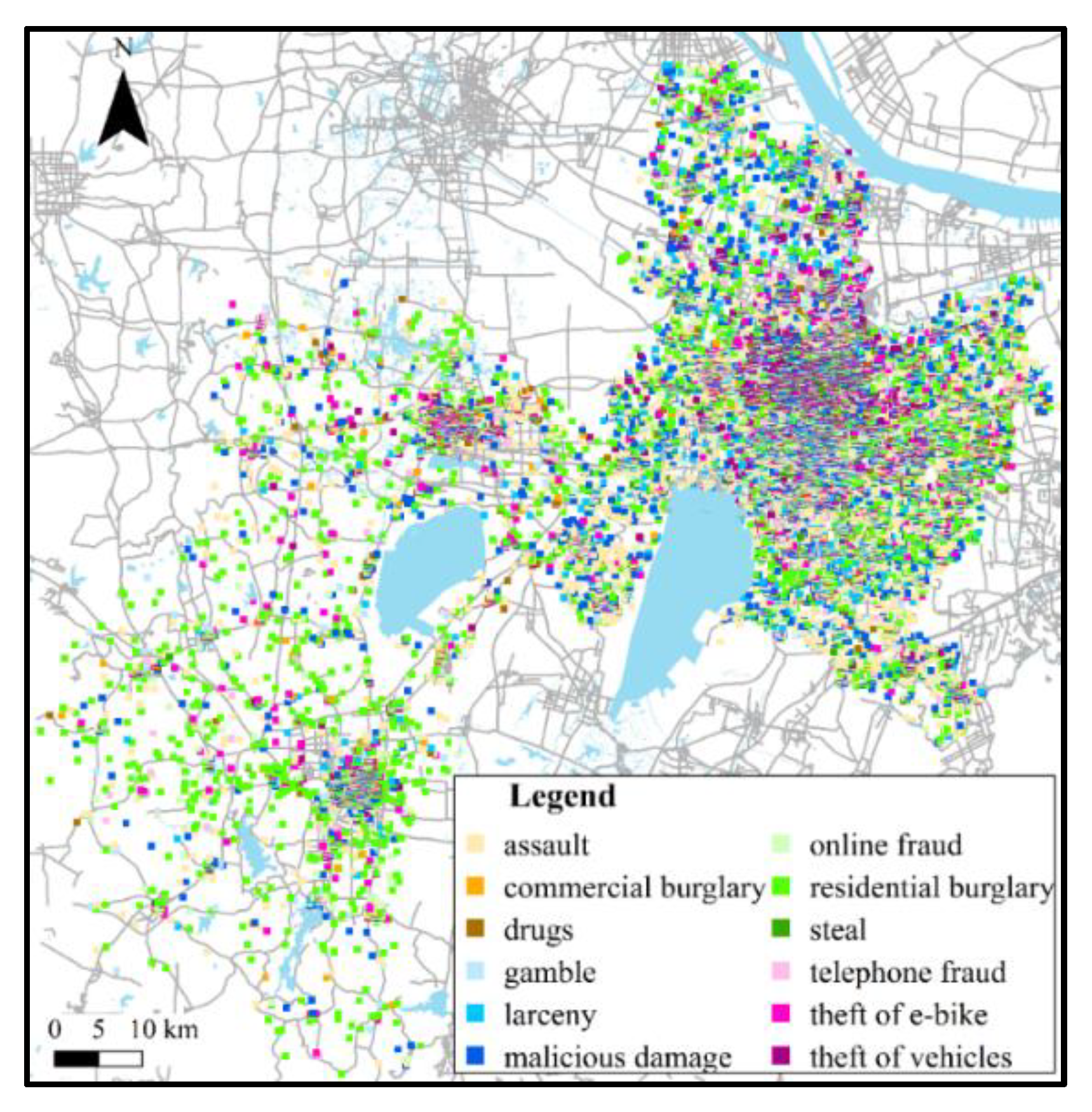
4.1. Real-World Crime Dataset Description

Our study area is located in the eastern part of the Yangtze River Delta and is one of the core cities of the UA-YRD. The study area is anonymized as X City in this study because of the confidentiality requirements imposed by the local Public Security Bureau. According to data from the National Bureau of Statistics of China [44], 5.2 million permanent residents and 1.8 million migrants live in X City. In addition, according to the China Statistical Yearbook [45], the rate of public security crimes in 2016 was the highest from 2016 to 2021, reaching 85 cases per 10,000 people. In 2016, the crime rate in the province in which X City is located ranked seventh in China [46]. Therefore, this study selected multiple types of public security crimes of X City in 2016 to verify the effectiveness of the proposed method.

The crime dataset includes twelve types of crimes in the study area, as shown in Figure 5. In this dataset, each crime event has complete information regarding the crime type, spatial occurrence location (latitude and longitude), and possible occurrence time interval. The spatial location was obtained by the police using GPS. The occurrence time interval was provided by the victims. The start and end times of the time interval were expressed in the form of year-month-day-hour-minute. The length of the time interval (i.e., the time span) implies the degree of the event’s occurrence time uncertainty. Thus, each crime event has relatively accurate location and semantic (e.g., crime type) information, but its time of occurrence has varying degrees of uncertainty.

Table 1. Numbers of crime events and percentages of events with different time spans.

ID	Type of Crime	Number of Events	Percentage of Events with Time Span
			<4 h	4–8 h	8–12 h	12–24 h
1	Assault	11,403	0.974	0.007	0.015	0.005
2	Commercial Burglary	1284	0.250	0.177	0.390	0.183
3	Drugs	1698	0.785	0.057	0.036	0.122
4	Gambling	1397	0.890	0.054	0.019	0.037
5	Larceny	3349	0.540	0.130	0.162	0.168
6	Malicious Damage	8040	0.508	0.096	0.186	0.209
7	Online Fraud	3471	0.729	0.116	0.051	0.104
8	Residential Burglary	8065	0.353	0.288	0.248	0.111
9	Stealing	2108	0.970	0.020	0.007	0.003
10	Telephone Fraud	2117	0.667	0.148	0.038	0.148
11	Theft of E-bike	6353	0.468	0.185	0.199	0.148
12	Theft of Vehicles	5639	0.330	0.154	0.243	0.273

lists the number of events and the time span distribution of the different types of crimes. The occurrence time uncertainty of assault, gambling, and stealing is relatively low. More than 80% of their events had a time span of less than 4 h. This is because these three types of crimes are more likely to be witnessed or experienced by the victims. Despite the relative accuracy of eyewitness experience, a certain degree of temporal uncertainty may result from the victim’s or witness’s biased recollection of the time of the occurrence. However, the occurrence time uncertainty of other types of crimes is relatively high, particularly theft of vehicles, commercial burglary, and residential burglary. For them, the percentage values of events with different time spans are insignificantly different, and the percentage with a time span of less than 4 h is not greater than 40%.

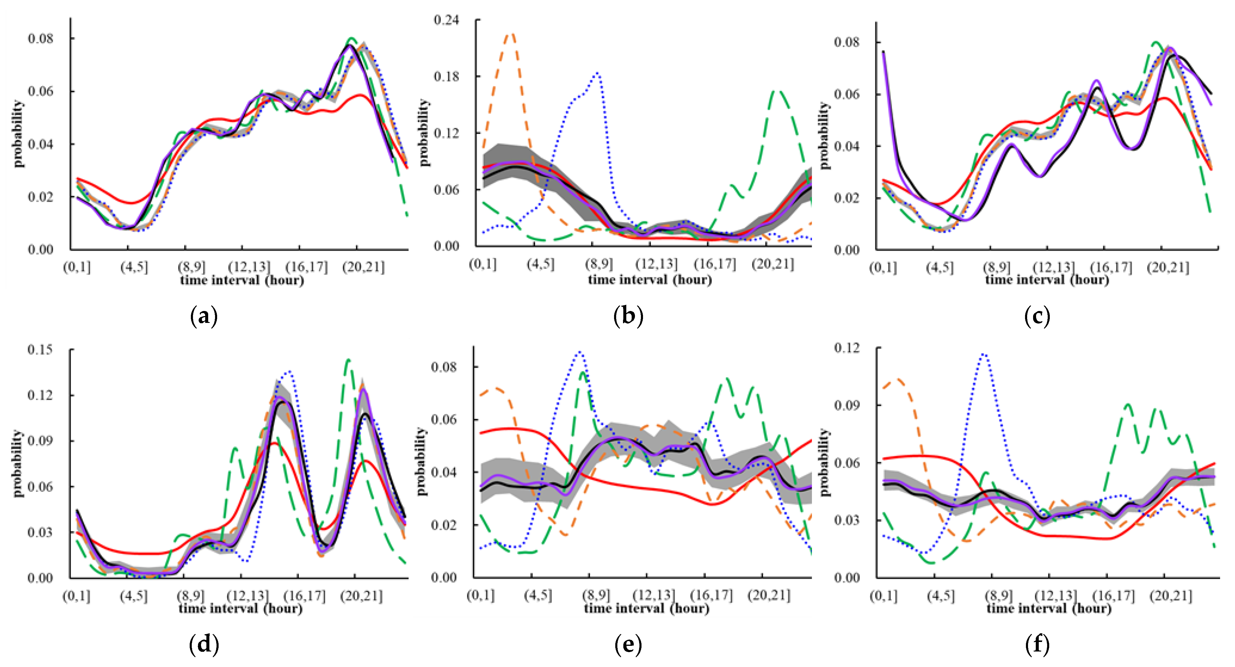
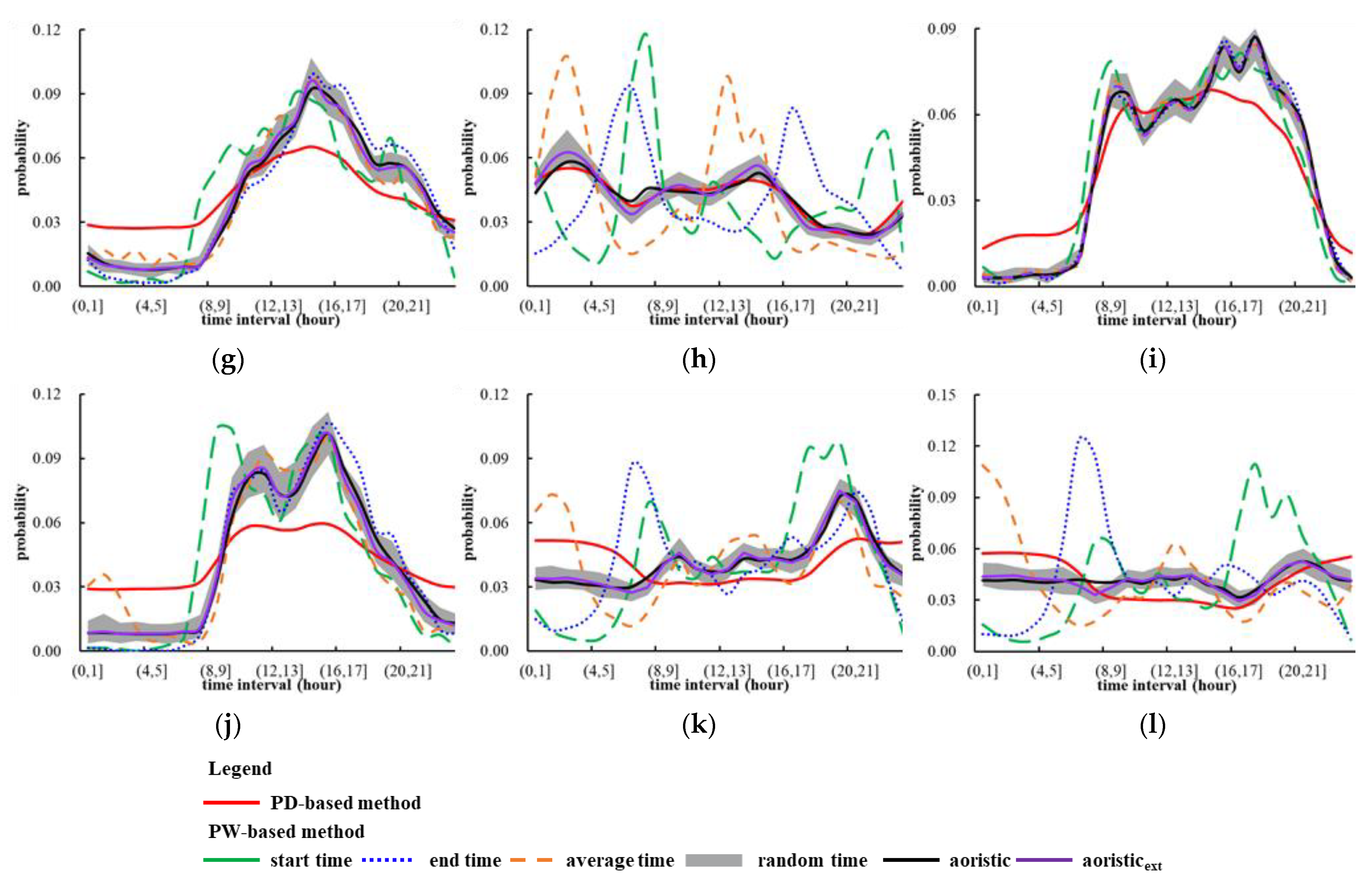
4.2. Experimental Comparisons of Crime Occurrence Time Modeling

Accurately modeling the occurrence time of crimes is the premise for the discovery of reliable USTCPs. In this section, we compare and analyze the occurrence probability distribution of crimes in the times obtained by the PD-based and PW-based methods. The length of the time slots is set to one hour for aoristic and aoristic_ext methods, according to the suggestions in [33]. The time resolution of the experimental dataset is one minute. Therefore, for the PD-based method, the temporal analysis scale r is set to one minute. In a day unit, the probability of twelve types of crimes occurring in different time intervals is generated using two methods, as shown in Figure 6. Note that the temporal probability distribution under the random time expression is a probability distribution range derived from 99 random samplings in the possible time interval.

As shown in Figure 6, the lower the time uncertainty, the more similar the probability distribution obtained by the two methods, such as the probability curves of assault, gambling, and stealing, as shown in Figure 6a,d,i, respectively. Furthermore, we observed that the start, end, and average times essentially reflect the daily activities of the victim. None of these can objectively characterize the temporal distribution of the crime events. Taking the commercial burglary in Figure 6b as an example, the crime has a noticeable peak between 20:00 and 21:00 when using the start time expression and a peak period from 8:00 to 9:00 when using the end time expression. Shop owners usually close their shops around 20:00 and 21:00 and then open the shops around 8:00 and 9:00 to find that burglary has occurred; thus, commercial burglary has a peak period around midnight under the average time expression. For most types of crimes, the trends of the probability curves generated by the PD-based, random time, aoristic, and aoristic_ext methods are similar. The latter three methods assume that events are independent and that the occurrence probability within the time interval is uniformly distributed. On this basis, for crimes with high time uncertainty, the probability curves obtained by these three methods have larger values if events with small time spans are concentrated. The ignorance of the temporal dependence of crime events could lead to an inability to objectively characterize the occurrence time of crime events. For example, in Figure 6e, larceny has a higher incidence from 8:00 to 9:00 under the random time, aoristic, and aoristic_ext expressions, whereas the PD-based method considers that the peak appears at 2:00–3:00. By analyzing the experimental dataset, 1136 larceny events were expected to appear around 2:00, and 965 larceny events may appear around 8:00. Therefore, assuming that a larceny event is more likely to appear between 2:00 and 3:00 is reasonable. The PD-based method fully uses the advantage of the kernel density estimation method, considering the dependence of geographical entities to obtain a stable temporal probability distribution, and it can eliminate the influence of some factors, such as the influence of the opening and closing times of the shops.

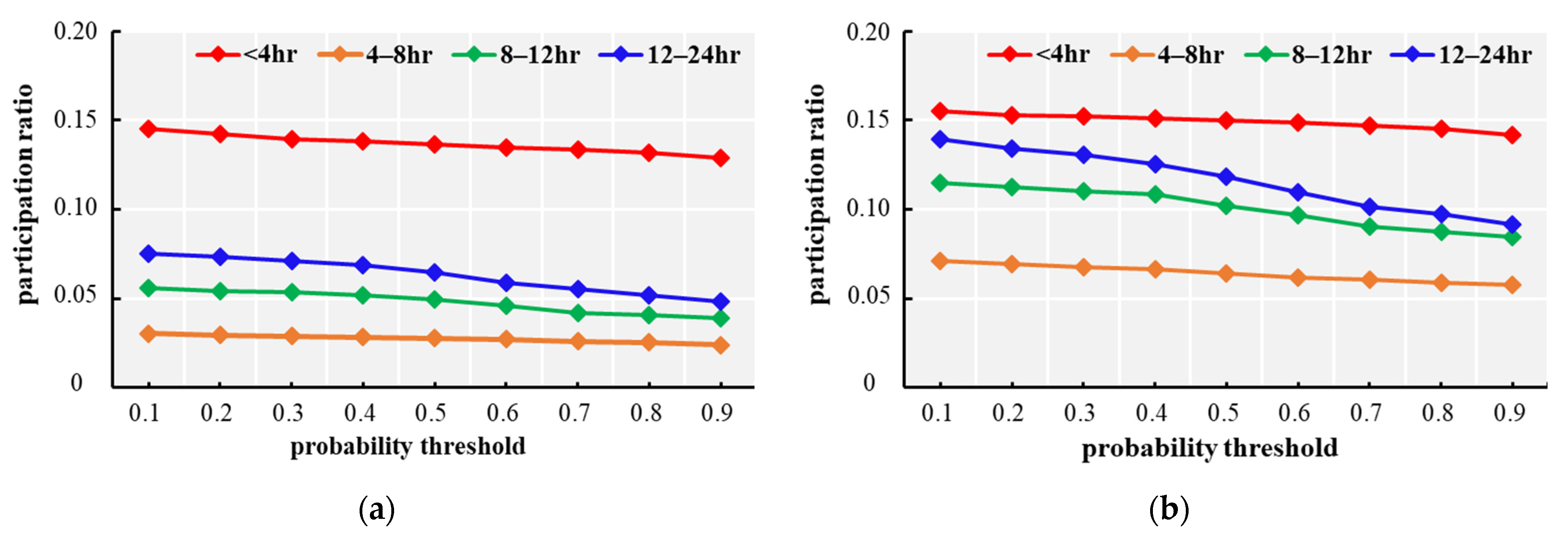
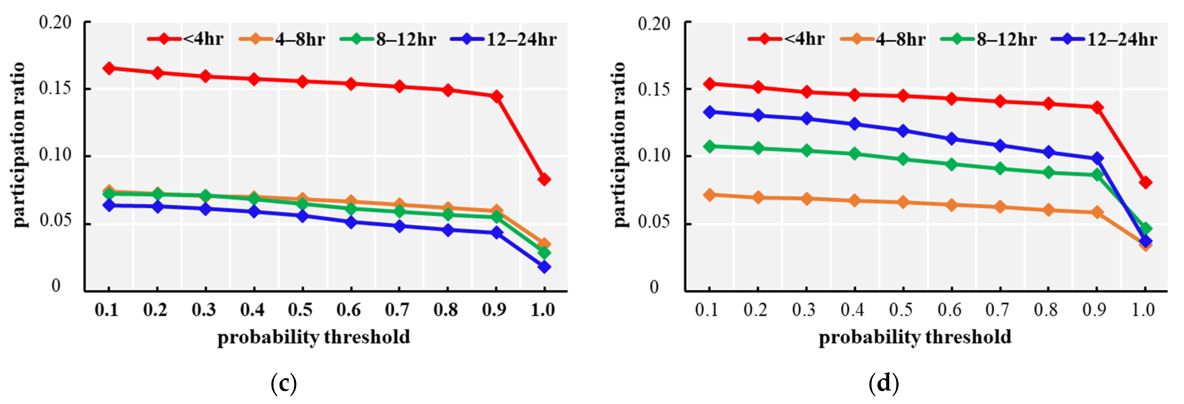
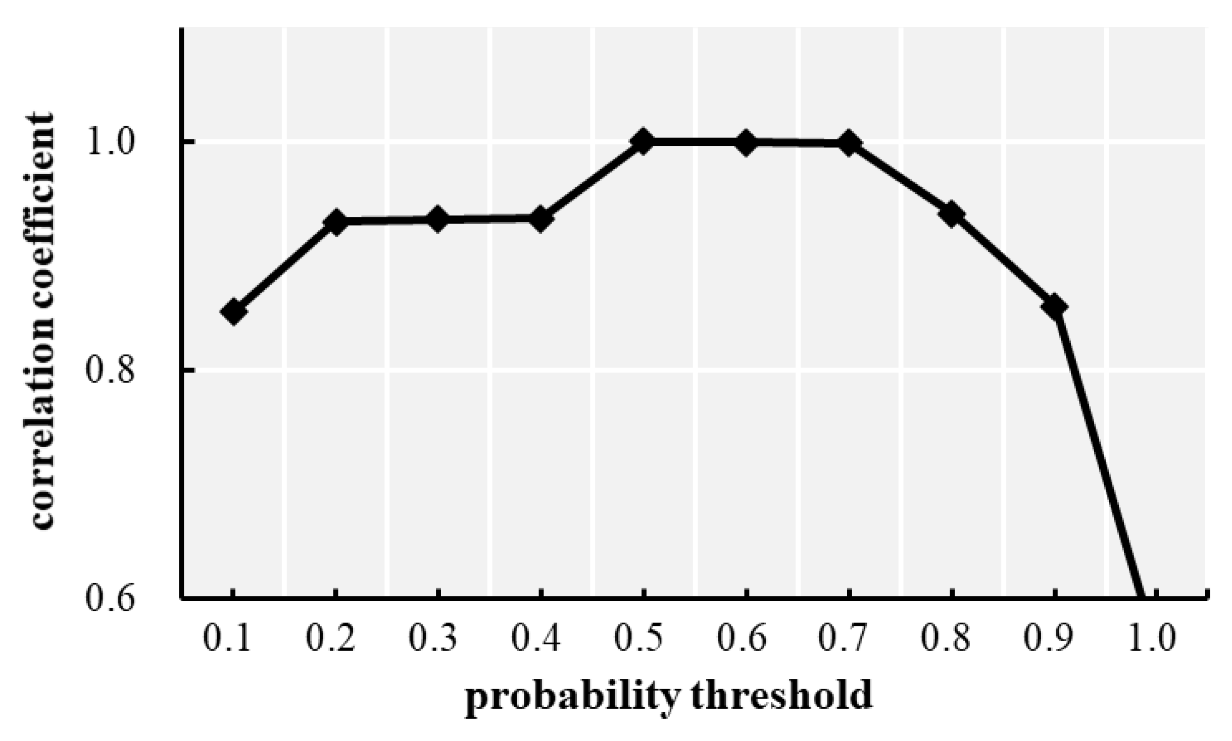
4.3. Analysis of USTCPs Discovered in the Crime Dataset

Referring to existing studies on the discovery of STCPs in the field of criminology [22,23], the spatial and temporal distance thresholds of the three methods are set to 1500 m and one day, respectively, and the prevalence threshold is set to 0.15. For the PD-based method, the probability threshold is set as 0.1–1 in increments of 0.1. The partial results for the USTCPs discovered using the three methods are presented in

Table 2. Participation index values of USTCPs obtained using the three methods.

USTCPs	PD-Based Method				PW-Based Method						ED-Based Method
	Probability Threshold				Start Time	Average Time	End Time	Random Time	Aoristic	Aoristicext
	0.1	0.5	0.8	0.9
{Assault, Larceny}	0.17	0.16	0.15	0.15	0.16	0.16	0.16	0.16	0.16	0.16	0.16
{Assault, Malicious Damage}	0.29	0.28	0.27	0.26	0.28	0.28	0.28	0.28	0.28	0.28	0.28
{Assault, Residential Burglary}	0.24	0.22	0.21	0.20	0.22	0.22	0.22	0.22	0.22	0.23	0.22
{Assault, Theft of E-bike}	0.25	0.23	0.22	0.22	0.24	0.23	0.24	0.23	0.24	0.24	0.23
{Assault, Theft of Vehicles}	0.18	0.17	0.15	-	0.17	0.17	0.16	0.17	0.17	0.17	0.16
{Commercial Burglary, Stealing}	0.17	0.17	0.17	0.16	0.16	0.17	0.17	0.17	0.17	0.17	0.17
{Drugs, Stealing}	0.18	0.17	0.16	0.16	0.17	0.17	0.17	0.17	0.17	0.17	0.17
{Larceny, Malicious Damage}	0.20	0.18	0.17	0.16	0.19	0.18	0.18	0.18	0.19	0.19	0.18
{Larceny, Online Fraud}	0.19	0.17	0.16	0.15	0.17	0.17	0.17	0.17	0.17	0.17	0.17
{Larceny, Theft of Vehicles}	0.22	0.19	0.17	0.17	0.20	0.19	0.20	0.19	0.20	0.20	0.19
{Larceny, Theft of E-bike}	0.21	0.19	0.17	0.16	0.19	0.19	0.19	0.19	0.19	0.19	0.19
{Malicious Damage, Online Fraud}	0.21	0.19	0.18	0.17	0.19	0.19	0.20	0.19	0.20	0.20	0.19
{Malicious Damage, Residential Burglary}	0.28	0.25	0.23	0.22	0.25	0.25	0.25	0.25	0.26	0.26	0.25
{Malicious Damage, Stealing}	0.17	0.16	0.15	0.15	0.16	0.16	-	-	-	-	0.16
{Malicious Damage, Telephone Fraud}	0.15	-	-	-	-	-	-	-	-	-	-
{Malicious Damage, Theft of E-bike}	0.35	0.33	0.30	0.29	0.33	0.33	0.33	0.33	0.33	0.33	0.33
{Malicious Damage, Theft of Vehicles}	0.31	0.28	0.25	0.24	0.28	0.28	0.28	0.28	0.28	0.28	0.28
{Online Fraud, Stealing}	0.15	-	-	-	-	-	-	-	-	-	-
{Online Fraud, Telephone Fraud}	0.17	-	-	-	0.16	-	-	-	-	-	-
{Online Fraud, Theft of E-bike}	0.23	0.21	0.19	0.19	0.22	0.21	0.21	0.21	0.22	0.21	0.21
{Online Fraud, Theft of Vehicles}	0.26	0.23	0.21	0.20	0.23	0.23	0.23	0.23	0.23	0.23	0.23
{Residential Burglary, Theft of E-bike}	0.25	0.23	0.21	0.20	0.23	0.23	0.23	0.23	0.23	0.23	0.23
{Residential Burglary, Theft of Vehicles}	0.20	0.18	0.16	0.15	0.18	0.18	0.18	0.18	0.18	0.18	0.18
{Stealing, Telephone Fraud}	0.18	0.16	0.16	0.15	0.16	0.16	0.16	0.16	0.17	0.17	0.16
{Stealing, Theft of E-bike}	0.22	0.20	0.19	0.19	0.20	0.20	0.20	0.20	0.20	0.21	0.20
{Stealing, Theft of Vehicles}	0.21	0.20	0.19	0.19	0.20	0.20	0.20	0.20	0.20	0.20	0.20
{Telephone Fraud, Theft of E-bike}	0.19	0.17	0.15	-	0.17	0.17	0.17	0.17	0.17	0.17	0.17
{Telephone Fraud, Theft of Vehicles}	0.18	0.16	-	-	0.16	0.16	0.16	-	0.16	0.17	0.16
{Theft of E-bike, Theft of Vehicles}	0.38	0.34	0.31	0.30	0.35	0.35	0.35	0.34	0.35	0.35	0.35

. The supplementary document provides the complete results.

By analyzing the results in Table 2, the following conclusions can be drawn. First, the prevalence of USTCPs identified by the PD-based method evidently decreases as the probability threshold increases. This phenomenon is particularly obvious in the USTCPs involving crimes with high time uncertainty. For example, in Table 1 the two types of crimes, malicious damage and theft of vehicles, have a low percentage of events whose time span is less than 4 h, but have a significantly high percentage of events whose time span is greater than 12 h. The prevalence of USTCPs composed of malicious damage and theft of vehicles varies greatly under different probability thresholds, such as {Malicious Damage, Theft of Vehicles} and {Theft of E-bike, Theft of Vehicles}. For these two patterns, as shown in Figure 7, the longer the time span of the crime events, the faster the participation ratio of the crime in the USTCP decreases as the probability threshold increases. Therefore, the uncertainty of the occurrence time of crimes directly leads to the instability of the spatio-temporal proximity relationship between the crime events.

Additionally, as shown in Table 2, the results of some USTCPs discovered by the PW-based methods under different time expressions are conflicting. For example, {Malicious Damage, Stealing} is prevalent under the start and average time expression, but it will be filtered out under other time expressions. Moreover, {Online Fraud, Telephone Fraud} is reported as prevalent only under the start time expression. The PW-based method ignores the time dependence among the crime events, which will result in some crime events occurring together or separately by chance under different time expressions, with inconsistent conclusions. Taking {Online Fraud, Telephone Fraud} as an example, with regard to all the pairs of crime events satisfying the spatio-temporal neighbor relationship under the start time expression, approximately 8% of them have a temporal probabilistic distance of less than 0.5. However, under other time expressions, this pattern is non-prevalent due to the relatively rare existence of this accidental phenomenon. In contrast, the proposed method can more exactly measure the temporal distance and discover reliable USTCPs. As shown in the supplementary document, the proposed method identifies {Online Fraud, Telephone Fraud} as prevalent USTCPs when the probability threshold is less than 0.5.

As shown in Figure 8, the results obtained by the ED-based and PD-based methods are extremely similar under the conditions of the probability thresholds from 0.5 to 0.7 and are less similar in other cases. This proves that the expected distance is the aggregation of partial possible distances between the events. As shown in Figure 9, the ED-based method filters out almost all pairs of crime events whose temporal probabilistic distance is less than 0.5. For the PD-based method, the frequency of different types of crimes co-occurring is reduced with an increasing probability threshold. Therefore, when the probability threshold is μ < 0.5 or μ ≥ 0.8, the similarity of the results discovered by the two methods is low. In fact, the temporal distance calculated by the ED-based method is the expected distance between the center of the time interval and another crime event. The temporal distance between possible timestamps other than the central point is lost, which leads to the misjudgment of the spatio-temporal neighborhood relationship and further results in incorrect decisions. However, the proposed method can more reliably discover USTCPs by fully using the distance information between the crime events. For instance, in Table 2 and Table S1, the ED-based method recognizes {Online Fraud, Telephone Fraud} as a non-prevalent USTCP. However, the PD-based method concludes the opposite when the probability threshold is not greater than 0.4. In practice, economic crime will cause serious economic losses to victims once it has occurred. Therefore, {Online Fraud, Telephone Fraud} detected by the proposed method under the condition of a small probability threshold is still meaningful, as it can guide the government and public security to determine the temporal and spatial areas that require more police resources.

Furthermore, the prevalent USTCPs can be analyzed with criminology theories, such as rational choice theory [47], routine activity theory [48], and boost theory [3]. The rational choice and routine activity theories indicate that the spatio-temporal context impacts the distribution of crime occurrence. A spatio-temporal context is generally a potential generator or attractor for the occurrence of different types of crimes. The boost theory suggests that crime risk can be propagated among crime events. Therefore, different types of crimes with similar criminal opportunities are likely to co-occur. Based on the effective understanding of prevalent USTCPs, police strategies can be enforced on easily controlled or key crimes to reduce crime rates. For example, in Table 2, malicious damage frequently appears in different USTCPs and can be regarded as a key crime. Moreover, malicious damage is easy to control because its target objects are generally public facilities. Therefore, malicious damage can be intervened in (e.g., by patrolling public spaces) to prevent other types of crimes.

5. Conclusions and Future Work

This paper proposed a probabilistic-distance-based method to discover USTCPs among multiple types of crimes with uncertain occurrence times. The occurrence time of each crime event is expressed as a probability density function in the possible time interval by considering the temporal dependence. This method can adaptively model the temporal uncertainty without a predefined probability distribution function. A probabilistic distance measurement is introduced to describe the temporal relationship among crime events, which comprehensively exploits the possible distance between crime events. The spatio-temporal neighborhood relationship based on the probabilistic distance can further improve the reliability of the discovered USTCPs. The experimental results of implementing the proposed method and the two types of existing methods on a real crime dataset demonstrate that the proposed method is superior and practical for crime event occurrence time uncertainty modeling and USTCP detection.

Future studies should focus on addressing the three limitations of this study. First, the spatio-temporal co-occurrence patterns among different types of crimes could be induced by the distribution characteristics of each crime type [22]. Such univariate distribution characteristics will be explored individually to explain the formation mechanism of USTCPs. Second, in practice, different types of crimes may co-occur even if no significant dependence exists among them. The null hypothesis of independence [49] should be further tested to identify more meaningful USTCPs with statistically significant dependence. Finally, we plan to explore the applicability of the proposed technique in a wider range of applications. For example, in epidemiology, USTCPs can contribute to a more accurate identification of factors influencing the spatial spread of COVID-19 by considering the uncertainty of the infection time of cases.

References

1. He, Z.; Deng, M.; Xie, Z.; Wu, L.; Chen, Z.; Pei, T. Discovering the joint influence of urban facilities on crime occurrence using spatial co-location pattern mining. Cities 2020, 99, 160612. [Google Scholar] [CrossRef]
2. Barnum, J.; Caplan, J.; Piza, E. The crime kaleidoscope: A cross-jurisdictional analysis of place features and crime in three urban environments. Appl. Geogr. 2017, 79, 203–211. [Google Scholar] [CrossRef] [Green Version]
3. Wang, Z.L.; Zhang, H. Could Crime Risk Be Propagated across Crime Types? ISPRS Int. J. Geo Inf. 2019, 8, 203. [Google Scholar] [CrossRef] [Green Version]
4. Golmohammadi, J.; Xie, Y.; Gupta, J.; Farhadloo, M.; Li, Y.; Cai, J.; Detor, S.; Roh, A.; Shekhar, S. An Introduction to spatial data mining. In The Geographic Information Science and Technology Body of Knowledge, 4th ed.; Wilson, J.P., Ed.; UCGIS: Ithaca, New York, USA, 2020. [Google Scholar]
5. Ratcliffe, J.H. Aoristic signatures and the spatio-temporal analysis of high volume crime patterns. J. Quant. Criminol. 2002, 18, 23–43. [Google Scholar] [CrossRef]
6. Martin, B.; Anton, B. Evaluating temporal analysis methods using residential burglary data. ISPRS Int. J. Geo Inf. 2016, 5, 148. [Google Scholar]
7. Lu, Y.; Wang, L.; Zhang, X. Mining frequent co-location patterns from uncertain data. J. Front. Comp. Sci. Technol. 2009, 3, 656–664. [Google Scholar]
8. Wang, L.; Wu, P.; Chen, H. Finding probabilistic prevalent colocations in spatially uncertain data sets. IEEE Trans. Knowl. Data Eng. 2013, 25, 790–804. [Google Scholar] [CrossRef]
9. Liu, Z.; Huang, Y. Mining co-locations under uncertainty. In Proceedings of the 13th International Conference on Advances in Spatial and Temporal Databases, Munich, Germany, 21–23 August 2013; pp. 429–446. [Google Scholar]
10. Tobler, W.R. A computer movie simulating urban growth in the Detroit region. Econ. Geogr. 1970, 46, 234–240. [Google Scholar] [CrossRef]
11. Chen, K.; Deng, M.; Shi, Y. A temporal directed graph convolution network for traffic forecasting using taxi trajectory data. ISPRS Int. J. Geo-Inf. 2021, 10, 624. [Google Scholar] [CrossRef]
12. Agrawal, R.; Srikant, R. Fast algorithms for mining association rules. In Proceedings of the 20th International Conference on Very Large Data Base, Santiago, Chile, 12–15 September 1994; pp. 487–499. [Google Scholar]
13. Yoo, J.S.; Shekhar, S. A joinless approach for mining spatial colocation patterns. IEEE Trans. Knowl. Data Eng. 2006, 18, 1323–1337. [Google Scholar]
14. Cai, J.; Deng, M.; Guo, Y.; Xie, Y.; Shekhar, S. Discovering regions of anomalous spatial co-locations. Int. J. Geogr. Inf. Sci. 2021, 35, 974–998. [Google Scholar] [CrossRef]
15. Shekhar, S.; Jiang, Z.; Ali, R.Y.; Eftelioglu, E.; Tang, X.; Gunturi, V.M.; Zhou, X. Spatiotemporal data mining: A computational perspective. ISPRS Int. J. Geo-Inf. 2015, 4, 2306–2338. [Google Scholar] [CrossRef]
16. Nakaya, T.; Yano, K. Visualising crime clusters in a space-time cube: An exploratory data-analysis approach using space-time kernel density estimation and scan statistics. Trans. GIS 2010, 14, 223–239. [Google Scholar] [CrossRef]
17. Koperski, K.; Han, J. Discovery of spatial association rules in geographic information databases. In Proceedings of the 4th International Symposium on Spatial Databases, Berlin, Germany, 6–9 August 1995; pp. 47–66. [Google Scholar]
18. Huang, Y.; Shekhar, S.; Xiong, H. Discovering colocation patterns from spatial data sets: A general approach. IEEE Trans. Knowl. Data Eng. 2004, 16, 1472–1485. [Google Scholar] [CrossRef] [Green Version]
19. Celik, M.; Shekhar, S.; Rogers, J.P.; Shine, J.A.; Yoo, J.S. Mixed-drove spatio-temporal co-occurrence pattern mining: A summary of results. In Proceedings of the 6th International Conference on Data Mining, Hong Kong, China, 18–22 December 2006; pp. 119–128. [Google Scholar]
20. Celik, M. Partial spatio-temporal co-occurrence pattern mining. Knowl. Inf. Syst. 2015, 44, 27–49. [Google Scholar] [CrossRef]
21. Qian, F.; Yin, L.; He, Q.; He, J. Mining spatio-temporal co-location patterns with weighted sliding window. In Proceedings of the 2009 IEEE International Conference on Intelligent Computing and Intelligent Systems, Shanghai, China, 20–22 November 2009; pp. 181–185. [Google Scholar]
22. Cai, J.; Deng, M.; Liu, Q.; Chen, Y.; He, Z.; Tang, J. A statistical method for detecting spatiotemporal co-occurrence patterns. Int. J. Geogr. Inf. Sci. 2019, 33, 967–990. [Google Scholar] [CrossRef]
23. Mohan, P.; Shekhar, S.; Shine, J.A.; Rogers, J.P. Cascading spatio-temporal pattern discovery. IEEE Trans. Knowl. Data Eng. 2011, 24, 1977–1992. [Google Scholar] [CrossRef]
24. Dalvi, N.; Dan, S. Management of probabilistic data: Foundations and challenges. In Proceedings of the 26th ACM Sigmod-Sigact-Sigart Symposium on Principles of Database Systems, Beijing, China, 11–13 June 2007; pp. 1–12. [Google Scholar]
25. Jiang, B.; Pei, J.; Member, S. Clustering uncertain data based on probability distribution similarity. IEEE Trans. Knowl. Data Eng. 2013, 25, 751–763. [Google Scholar] [CrossRef]
26. Wang, Z.; Lu, B.; Ying, F.; Kong, M.; Tang, M. Research of mining algorithms for uncertain spatio-temporal co-occurrence pattern. In Proceedings of the 9th International Conference on Knowledge and Smart Technology, Chonburi, Thailand, 1–4 February 2017; pp. 12–17. [Google Scholar]
27. Ngai, W.K.; Kao, B.; Chui, C.K.; Chen, R.; Chau, M.; Yip, K.Y. Efficient clustering of uncertain data. In Proceedings of the 6th International Conference on Data Mining, Hong Kong, China, 18–22 December 2006; pp. 436–445. [Google Scholar]
28. Gullo, F.; Ponti, G.; Tagarelli, A.; Greco, S. A hierarchical algorithm for clustering uncertain data via an information-theoretic approach. In Proceedings of the 8th IEEE International Conference on Data Mining, Washington, WA, USA, 15–19 December 2008; pp. 821–826. [Google Scholar]
29. Zhao, Z.; Yan, D.; Ng, W. Mining probabilistically frequent sequential patterns in large uncertain databases. IEEE Trans. Knowl. Data Eng. 2014, 26, 1171–1184. [Google Scholar] [CrossRef]
30. Ahmed, A.U.; Ahmed, C.F.; Samiullah, M.; Adnan, N.; Leung, K.S. Mining interesting patterns from uncertain databases. Inf. Sci. 2016, 354, 60–85. [Google Scholar] [CrossRef]
31. Sun, L.; Cheng, R.; Cheung, D.W.; Cheng, J. Mining uncertain data with probabilistic guarantees. In Proceedings of the 16th ACM SIGKDD International Conference on Knowledge Discovery and Data Mining, Washington, WA, USA, 25–28 July 2010; pp. 273–282. [Google Scholar]
32. Ashby, M.P.; Bowers, K.J. A comparison of methods for temporal analysis of aoristic crime. Crime Sci. 2013, 2, 1. [Google Scholar] [CrossRef] [Green Version]
33. Oswald, L.; Leitner, M. Evaluating temporal approximation methods using burglary data. ISPRS Int. J. Geo-Inf. 2020, 9, 386. [Google Scholar] [CrossRef]
34. Lu, H.; Han, J.; Feng, L. Stock movement prediction and n-dimensional inter-transaction association rules. In Proceedings of the SIGMOD Workshop, Research Issues on Data Mining and Knowledge Discovery, Washington, WA, USA, 13 June 1998; pp. 1–7. [Google Scholar]
35. Wang, Z.; Hong, Z. Construction, detection, and interpretation of crime patterns over space and time. ISPRS Int. J. Geo-Inf. 2020, 9, 339. [Google Scholar] [CrossRef]
36. Liu, H.; Zhang, X.; Zhang, X.; Cui, Y. Self-adapted mixture distance measure for clustering uncertain data. Knowl. Based Syst. 2017, 126, 33–47. [Google Scholar] [CrossRef]
37. Wiegand, T.; Moloney, K.A. Handbook of Spatial Point-Pattern Analysis in Ecology; CRC Press: Boca Raton, FL, USA, 2013; pp. 94–98. [Google Scholar]
38. Yue, H.; Zhu, X.; Ye, X.; Guo, W. The local colocation patterns of crime and land-use features in Wuhan, China. ISPRS Int. J. Geo-Inf. 2017, 6, 307. [Google Scholar] [CrossRef] [Green Version]
39. Felson, M.; Poulsen, E. Simple indicators of crime by time of day. Int. J. Forecast. 2003, 19, 595–601. [Google Scholar] [CrossRef]
40. Xu, C.; Liu, L.; Zhou, S.; Ye, X.; Jiang, C. The spatio-temporal patterns of street robbery in DP peninsula. Acta Geogr. Sinica 2013, 68, 1714–1723. [Google Scholar]
41. Silverman, B.W. Density Estimation for Statistics and Data Analysis; Chapman and Hall: Boca Raton, FL, USA, 1986; p. 46. [Google Scholar]
42. Zhang, X.; Liu, H.; Zhang, X. Novel density-based and hierarchical density-based clustering algorithms for uncertain data. Neural Netw. 2017, 93, 240–255. [Google Scholar] [CrossRef]
43. Shekhar, S.; Huang, Y. Discovering spatial co-location patterns: A summary of results. In Proceedings of the International Symposium on Spatial and Temporal Databases, Redondo Beach, CA, USA, 12–15 July 2001; pp. 236–256. [Google Scholar]
44. National Bureau of Statistics of China. China Population Census Yearbook 2020; China Statistics Press: Beijing, China, 2020.
45. National Bureau of Statistics of China. China Population Statistical Yearbook 2017; China Statistics Press: Beijing, China, 2017.
46. The Supreme People’s Procuratorate of China. Procuratorial Yearbook of China 2017; China Procuratorate Press: Beijing, China, 2017.
47. Becker, G.S. Crime and punishment: An economic approach. J. Polit. Econ. 1968, 76, 169–217. [Google Scholar] [CrossRef] [Green Version]
48. Cohen, L.E.; Felson, M. Social change and crime rate trends: A routine activity approach. Am. Soc. Rev. 1979, 44, 588–608. [Google Scholar] [CrossRef]
49. Cai, J.; Kwan, M.P. Discovering co-location patterns in multivariate spatial flow data. Int. J. Geogr. Inf. Sci. 2022, 36, 720–748. [Google Scholar] [CrossRef]
Figure 1. Crime dataset.
Ijgi 11 00454 g001
Figure 2. Two possible worlds of the uncertain dataset in Figure 1: (a) a possible world under start time expression and (b) a possible world under end time expression.
Ijgi 11 00454 g002
Figure 3. Example of the modeling of the temporal probability density function of crime events: (a) a crime dataset; (b) the frequency of timestamps in POTk; (c) temporal population distribution of Ck; and (d) the temporal probability density function of the three events.
Ijgi 11 00454 g003
Figure 4. Example of constructing spatio-temporal neighborhood relationships: (a) relationship constructed using the expected-distance-based method and (b) relationship constructed using the probabilistic-distance-based method.
Ijgi 11 00454 g004
Figure 5. Spatial distribution of all categories of crimes.
Ijgi 11 00454 g005
Figure 6. Probability of all types of crimes occurring in different time intervals generated by two methods: (a) assault, (b) commercial burglary, (c) drugs, (d) gambling, (e) larceny, (f) malicious damage, (g) online fraud, (h) residential burglary, (i) stealing, (j) telephone fraud, (k) theft of e-bikes, and (l) theft of vehicles.
Ijgi 11 00454 g006aIjgi 11 00454 g006b
Figure 7. Participation ratio values of crimes with different time spans participating in the USTCPs: (a,b) the participation ratio values of malicious damage and theft of vehicles participating in {Malicious Damage, Theft of Vehicles}; (c,d) the participation ratio values of theft of e-bike and vehicles events participating in {Theft of E-bike, Theft of Vehicles}.
Ijgi 11 00454 g007aIjgi 11 00454 g007b
Figure 8. Pearson correlation coefficient of the participation index sequences generated by the PD-based method at different probability thresholds and by the ED-based method.
Ijgi 11 00454 g008
Figure 9. Number of co-occurrence instances of {Telephone Fraud, Theft of Vehicles} located in different temporal probabilistic distance intervals obtained by ED-based and PD-based methods (μ = 0.1).
Ijgi 11 00454 g009