RDQS: A Geospatial Data Analysis System for Improving Roads Directionality Quality

Abstract

With the increasing availability of smart devices, billions of users are currently relying on map services for many fundamental daily tasks such as obtaining directions and getting routes. It is becoming more and more important to verify the quality and consistency of route data presented by different map providers. However, verifying this consistency manually is a very time-consuming task. To address this problem, in this paper we introduce a novel geospatial data analysis system that is based on road directionality. We investigate our Road Directionality Quality System (RDQS) using multiple map providers, including: Bing Maps, Google Maps, and OpenStreetMap. Results from the experiments conducted show that our detection neural network is able to detect an arrow’s position and direction in map images with >90% F1-Score across each of the different providers. We then utilize this model to analyze map images in six different regions. Our findings show that our approach can reliably assess map quality and discover discrepancies in road directionality across the different providers. We report the percentage of discrepancies found between map providers using this approach in a proposed study area. These results can help determine areas needs to be revised and prioritized to improve the overall quality of the data within maps.

1. Introduction

Digital maps are currently being used daily by millions of users. This usage has increased significantly in the last decade due to the huge surge in availability of smart devices. Google Maps alone is estimated to have more than a billion monthly active users [1]. It is becoming more and more important for map providers to provide high accuracy for their maps. Despite the high accuracy already achieved by the main map providers, they are still far from perfect. Many researches focusing on analyzing map data quality, such as [2,3,4], report discrepancies in different aspects of the data. One of the existing challenges across map providers is that while all of them support the directionality of roads, those directions are not necessarily consistent. Because each provider uses different methodologies, there are discrepancies between the maps provided. While some discrepancies might cause inconvenience to users, other discrepancies such as wrong road directions might pose some serious risks. While providers take great care to avoid giving wrong directions, this is a costly endeavor. Our system dramatically reduces these costs by highlighting areas in which errors are likely to exist.

In this paper, we present RDNN, a road directionality neural network model that detects arrows and classifies their directionality with high accuracy across three map providers including: (a) Google Maps, (b) Bing Maps, and (c) OpenStreetMap (OSM). We measure and report accuracy rates achieved for the different providers. Then we utilize this model to scan and analyze large areas to discover potential discrepancies in road directionality. To illustrate the importance of detecting arrow directionality, consider Figure 1 which shows a cross section of the same geographic location across two providers (Google Maps and Bing Maps) but having completely different arrows’ directionality. As can be seen in Figure 1, Bing Maps’ image has an arrow pointing southeast, while Google Maps’ image arrow is pointing northwest. The mismatched arrow directionality illustrates the discrepancies that may occur and is an example of inaccurate information passed to end users that might pose a serious safety hazard. In such cases, it is not clear which of the two providers has accurate directionality for the examined road, but an error must exist in one of them. As maps are populated with more information, such discrepancies are becoming more common across map providers. Our system can detect these errors and report them for investigation.

Such inaccuracies may lead to possible accidents. For example, this mislabelling of the road directions may cause a driver who depends on map services for directions and navigation to attempt to drive in the wrong direction, which can be a serious safety hazard, possibly leading to road accidents. The matter may become even worse involving roads with dense traffic. This is an example of a discrepancy that our approach can automatically identify and report. By scanning large areas, we can then efficiently identify and report a larger segment of these discrepancies and aggregate statistical results that can help guide which areas contain a large percentage of discrepancies and need to be revised. This can significantly help cartographers in improving the overall quality of the maps that are proprietary (e.g., Google Maps, Bing Maps). While open-source maps such as OSM can significantly help correct these inaccuracies since end users are able to correct them, changes to other propriety maps such as Google Maps and Bing Maps require additional overhead or steps involving editorial teams to administer such changes.

In this paper, we contribute the following:

• We present RDNN, a road directionality neural network model that detects arrows’ directionality in map images across map providers with high accuracy.
• We conduct a series of experiments to measure and evaluate the accuracy of the detection model using a real-world maps dataset.
• We publish our training and test datasets used to train and evaluate the neural network to make it available for future works in this area.
• We present RDQS, a road directionality quality system that utilizes and integrates this model, along with other components, to assess the quality of maps and report discrepancies in road directionality.
• We conduct experiments utilizing this system to automatically scan thousands of locations in six major regions to identify and report discrepancies in road directionality discovered by our method.

1.1. Related Work

1.1.1. Road Segment Detection System

One important area for comparing discrepancies across map providers is road segments. Many providers have discrepancies in this area. Researchers at UW Tacoma [5] are developing a system that can detect roads from map images using computer vision. A group of color-based techniques and segmentation using k-means are used to filter images and extract binary and skeleton representation of road segments. Later, more information about the width and length of different road segments is extracted. This information is aggregated and used to provide statistics highlighting major discrepancies across providers in some areas. We utilize this work in our paper to build a full road network graph (RNG) including directions so we can compare the resulting RNG across different providers.

1.1.2. Road Network Graphs Using Routing API

A group of researchers investigated road network graphs across different providers by utilizing the routing APIs [6]. The approach was to randomly create routes from point A to point B and compare the different routes provided by different providers. If there is a discrepancy, this indicates a difference in the underlying mapping system and road segments for that area. For example, a missing road or a road labeled with the wrong direction in one provider might cause this provider to provide a route that is significantly more expensive than the one provided by a different provider.

We are following a different approach by using computer vision to extract arrow directions information and utilize that to discover these discrepancies.

1.1.3. Road Network Detection Using Probabilistic and Graph Theoretical Methods

Researchers in [7] propose an automated system to detect road networks from satellite and aerial images for the purpose of map generation. The methodology depends on probabilistic road center detection and graph-theory-based road network information. The results achieved indicate the system can be used in detecting road networks on satellite images. Our approach is different in that we focus on road directionality by detecting arrows’ locations and directionality from map images.

1.1.4. Vision-Based Traffic Light and Arrow Detection

In this paper [8], researchers proposed a vision-based detection algorithm for traffic lights. It detects all three traffic lights including arrow direction. The system can be used for intelligent vehicles. The system uses a convolutional neural network that is fine-tuned for varying traffic lights and illumination conditions. However, this research only focuses on detecting arrows in the context of traffic lights and only detects three directions: left, right, and forward. It does not address arrow multi-directionality detection in map images across different providers, which is what we are focusing on in this paper.

1.1.5. Arrow Detection in Medical Images

Researchers in [9] built a model for detecting arrows used to label medical images to help improve their analysis of regions of interest for their content-based image retrieval. They used key point detection to identify the vertices of the arrowhead, while ignoring the arrow’s base. They then used four layers of binarization of the image’s gray-scale to help filter out noise and distinguish between overlapping arrows. Ultimately, their goal was to use these detected arrows to find significant parts of an image to focus on processing for information retrieval. Our own arrow detection, however, is not intended for image content retrieval but is instead intended to help identify potential errors in map providers.

1.1.6. Arrow Detection in Handwritten Diagrams

The authors in [10] used a proposed modification of Faster R-CNN called Arrow R-CNN to analyze hand-drawn flowchart diagrams. Their Arrow R-CNN modifies Faster R-CNN by using Feature Pyramid Networks and key point detection, labeling their arrow’s heads and tails. It is interesting that they used their arrow detection as the basis for reconstructing digital versions of hand-drawn diagrams, while we intend to use our own arrow detection to develop a road network graph. A key difference is that for them, the arrows serve as the connections between parts of a flowchart, while for us, it is the roads that connect our graph with the arrows being used to tell the direction of the edges. For that reason, being able to determine the directionality of our arrows is critically important.

1.1.7. State-of-the-Art Deep Learning Models in Computer Vision

The main deep learning algorithm used for computer vision tasks is Convolutional Neural Networks (CNN). CNNs have had tremendous improvements in recent years improving object detection performance significantly on main benchmark datasets. They also, until very recently, have been forming the backbone of state-of-the-art models in computer vision domain. One of the latest improvements was the introduction of Fast R-CNN [11] and Faster R-CNN [12]. Faster R-CNN achieved state-of-the-art performance [12] at the time the paper was published for object detection and semantic segmentation tasks on the COCO dataset [13], which is the current standard dataset used for comparing models for object detection tasks. Faster R-CNN continues to be the backbone of models with one of the best results in the computer vision domain.

Very recently in 2021, the computer vision domain is shifting with the introduction of transformer-based models for computer vision tasks such as ViT [14]. Although ViT shows promising results for solving simple classification tasks, it failed to generalize well for more complex tasks such as object detection and semantic segmentation due to the fixed 16 × 16 batch size. Moreover, time increases quadratically with image size increase. This makes real-time inference a real challenge with ViT. Improvements on ViT to address these challenges led to the introduction of Swin Transformer [15]. Swin Transformer uses a shifted window with limited attention to be able to capture features at different scales. Based on the Swin Transformer paper [15], it achieves state-of-the-art results for object detection tasks on the COCO dataset [13]. The converging of transformers into the computer vision domain is still very new and a very active field of study. A very recent paper named “A ConvNet for the 2020s” [16] reemphasized the importance of convolutions in computer vision and introduced a family of models called ConvNeXts. ConvNeXts are standard ConvNet models modernized towards the design of a hierarchical vision Transformer (Swin). That is, the idea is to adapt techniques from transformers into a native convolution architecture to realize the benefits that transformers bring, while maintaining the simplicity and efficiency of a convnet architecture. The paper shows that ConvNeXts compete favorably with the Swin Transfomer in common computer vision tasks such as object detection and semantic segmentation.

In this paper, we use Faster R-CNN based models provided by the Detectron2 library [13]. Detectron2 provides models with one of the best results and near state-of-the-art performance for many computer vision tasks as well. One of the main reasons for this choice is the amount of available resources, documentation, examples, and frameworks supporting utilizing these models compared to transformer-based models which were very recently introduced. Moreover, the objects we detect (arrows) in this paper are extremely small. ViT has major problems with detecting small features in images due to its fixed 16 × 16 batch size. Swin Transformer supposedly addresses this problem with the shifting window approach. However, it is not clear if this going to be good enough for detecting extremely small objects (composed of a few pixels) such as arrows. Faster R-CNN models have a known stable architecture for detecting features at different scales. Moreover, we find Faster R-CNN models very easy to work with and easy to retrain. In addition, it achieves sufficient results for the purpose of this paper as we present later. Using Swin Transformer for this task is definitely interesting, but it is beyond the scope of this paper and may be a potential area we investigate in future works.

1.1.8. Additional Related Work

Given the importance of accuracy of spatial data in maps, many map features have been studied in detail, such as evaluating the relative accuracy of lane lines for high-definition maps (HDM) for autonomous driving (AD) [17] and matching entities in different data sources for residential areas [18].

Other researchers investigated the quality of semantic information such as road type associated with data in OpenStreetMap (OSM) [19]. Researchers in this paper proposed an approach using supervised machine learning to assess the quality of spatial data provided through Volunteered Geographic Information (VGI) based on analyzing specific features (characteristics) of the data. Many other studies focused on the quality of several other features of OSM such as road networks [20,21,22], street names [23], POIs [2], road names [24], and routing ways [25].

However, none of these studies focuses on the quality of directionality and compares the quality of this data across different providers such as OSM, Google Maps, and Bing Maps, which is the focus in this paper.

1.1.9. Comparisons to Other Work

There has been research conducted to detect arrows in physical road markings [26] and traffic lights [8], and there has been research undertaken to detect arrows symbols in flowcharts [10] and in medical diagrams [9], but our work focuses on training a model to detect and classify arrow symbols on online maps, which seems to be a mostly unexplored application of computer vision. While there are other researchers comparing features of different map providers [5], to our knowledge, we are the only ones comparing map arrow directions. While some researchers have studied creating road network graphs by extracting road segments from maps [5], and others have created them by analyzing satellite imagery [7], we remain unique in our ability to use arrow direction detection in creating multi-directional graphs.

Table 1. Comparison of related work.

Paper	Methodlogy	Builds RNG	Detects Arrows	Multi-Directionality	Arrow Source	Compares Providers
Road Segment [5]	Binarization	NO	NO	NO	N/A	YES
Routing API [6]	Uses Routing APIs	YES	NO	NO	N/A	YES
Satellite Road Network [7]	Probabilistic Methods	YES	NO	NO	N/A	NO
Traffic Light [8]	CNN	NO	YES	YES	Traffic Lights	NO
Medical Images [9]	Template Comparison	NO	YES	NO	Medical Images	NO
Arrow R-CNN [10]	Arrow RCNN	NO	YES	NO	Flowcharts	NO
RDNN (this paper)	Faster RCNN	YES	YES	YES	Online Maps	YES

summarizes the differences between our approach and other related work.

2. Materials and Methods

Our goal is to detect arrow directionality with high accuracy across different map providers. We utilize Detectron2 [13], which is a library that provides state-of-the-art collections of Fast R-CNN [11] and Faster R-CNN [12] neural networks for object detection. In Section 1.1.7 of related work, we present a more detailed discussion on the state-of-the-art deep learning models in computer vision and explain why we use this library. Fast R-CNN is an improvement over traditional R-CNN (regional-based convolutional neural network) methods. R-CNN uses a selective search algorithm to extract lists of region proposals, which are then fed to the network one by one. This makes the network very slow due to the generation of multiple region proposals that each need to be fed independently to the CNN for feature extractions. Moreover, the selective search algorithm is fixed and cannot be trained, which might lead to bad candidate region proposals on new classes of images which would be problematic given that training the model to recognize new classes of images is part of the goal of this research.

Faster R-CNN is an improvement over traditional R-CNN and Fast R-CNN since it eliminates the slow selective search algorithm and instead allows the network to learn the region proposals. As presented in Figure 2, Faster R-CNN essentially introduces a separate network to learn and predict the region proposals. Then these regions are fed to the detection network for object detection. This makes it faster and also more suitable for re-training on different classes since the region proposal network can also be re-trained as well.

For these advantages, we start with a pre-trained Faster R-CNN model from the Detectron2 library. The model we select is Faster R-CNN with ResNet-101 backbone and a feature pyramid network (FPN). This model achieved state-of-the-art results for object detection tasks when it was introduced [27]. The use of FPN makes it fast and very easy to re-train on new dataset. FPN also makes the model very good at detecting objects at different scales, which is extremely important for our purpose since we detect very small arrow objects in map images. The pre-trained model is trained on the COCO dataset [28] which has a total of 2.5 million labeled instances in 328 k images. Then, we prepare a new training dataset by labeling map images obtained by downloading images using APIs provided by the different providers. We freeze all layers in the neural network except the last one. The last layer is a fully connected layer. We use the training dataset to retrain the network and tune the weights of this last layer based on the new dataset. This gives us a network that detects the new desired classes (arrow directions).

Then, we quantify the accuracy of the network using a test dataset that is prepared in a similar fashion to the training dataset. We use AP (Average Precision) and AR (Average Recall) as our evaluation metrics. We use the intersection over union metric with a threshold of 0.5 (AP50 and AR50) to determine true positives. This means that if an area of the intersection of the predicted bounding box and the ground truth’s bounding box is more than half the size of the two combined bounding boxes, it is counted as a valid prediction.

$$IoU=\frac{AreaofOverlap}{AreaofUnion}$$

(1)

The training and test datasets use COCO [28] format. COCO is a popular format used in the object detection domain, and it is compatible with the Detectron2 library. Thus we use this format for all our experiments throughout this paper. AP and AR are the standard metrics to evaluate and report for COCO datasets which we use in this paper.

We note that detecting an arrow’s directionality in map images introduced in this paper is a novel effort. To our knowledge, it has not been undertaken before. Thus we do not have any baseline to compare the accuracy of our model to. Moreover, there is no standard dataset to be used as a benchmark. Thus as part of this effort, we publish our datasets and make them available as open source to help establish a baseline benchmark that can be utilized later on by any future work in this area.

Finally, after tuning this model, we utilize it in a bigger system we call RDQS (Road Directionality Quality System) that automatically downloads map images and analyzes these tiles using this model and other computer-vision based components to scan for discrepancies in road directionality and report overall stats for the different study areas.

In this section, we present the details of the architecture of the proposed system. At a high level, our road-directionality system architecture is presented in Figure 3.

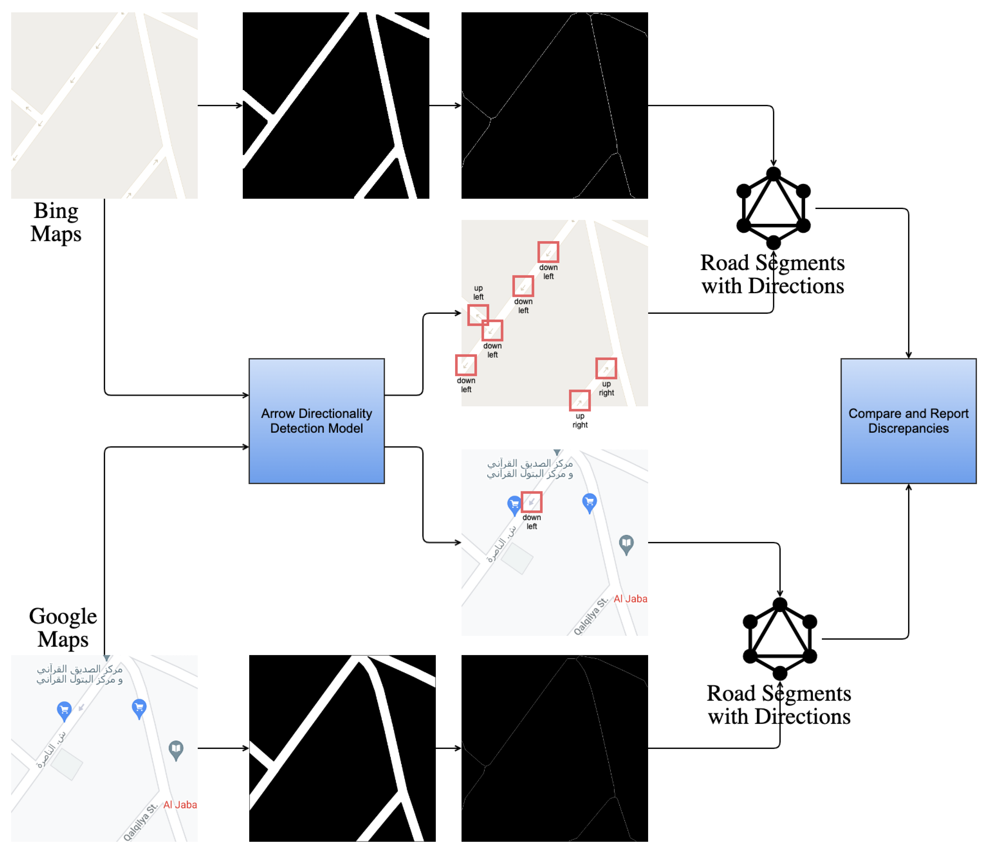
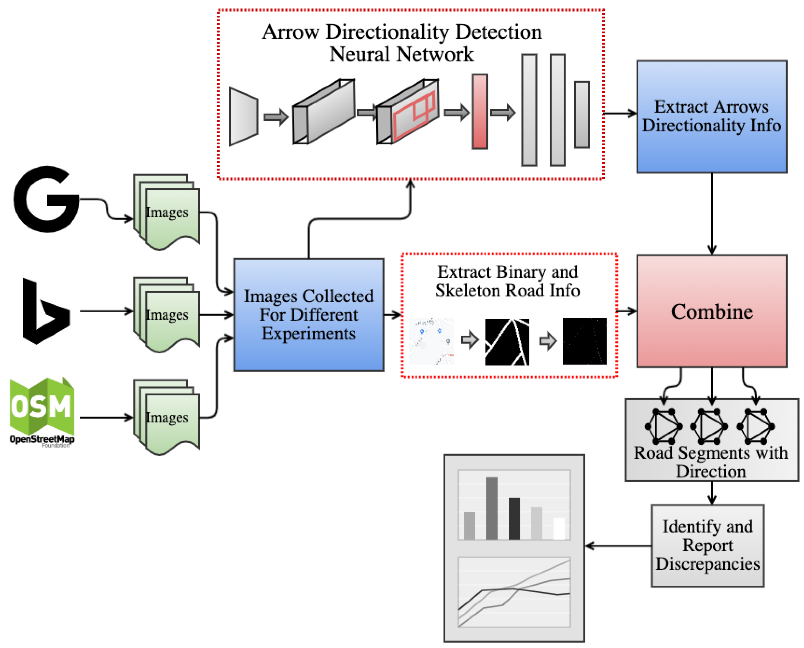
2.1. System Architecture

As can be seen in Figure 3, we collect images from Google Maps, Bing Maps, and OSM and feed them into the detection neural network model. The network detects both arrows’ locations and directionality. We also utilize a component from a paper published by University of Washington researchers [5] to extract binary and skeleton road segment information. We define road segments as road stretches between intersections. We then feed the road segment information along with the corresponding arrows directionality information to a component that overlays the two and matches every road segment with the arrow that belongs to it. This is performed per image for every provider. Then, we analyze the generated road segments for each image across the different providers and match corresponding road segments based on map locality. Finally, we compare and identify discrepancies in arrows’ directionality associated with matched road segments. Furthermore, we aggregate the results over the entire study area and report the degree to which such similarities and discrepancies occur.

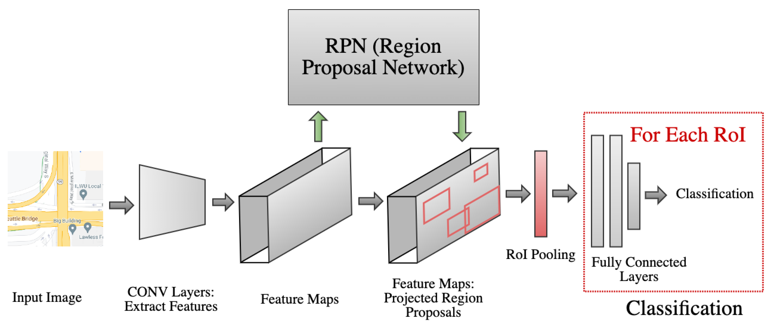
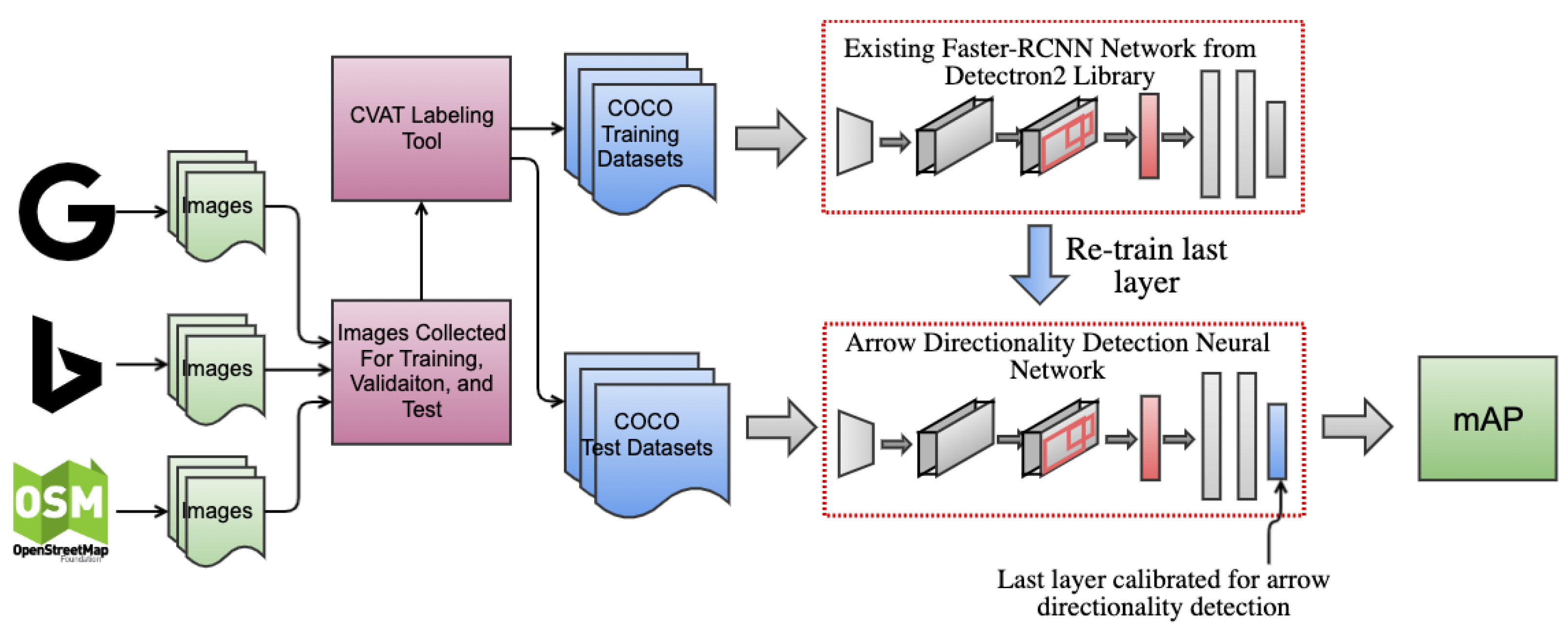
2.2. Road-Directionality Neural Network Model Overview

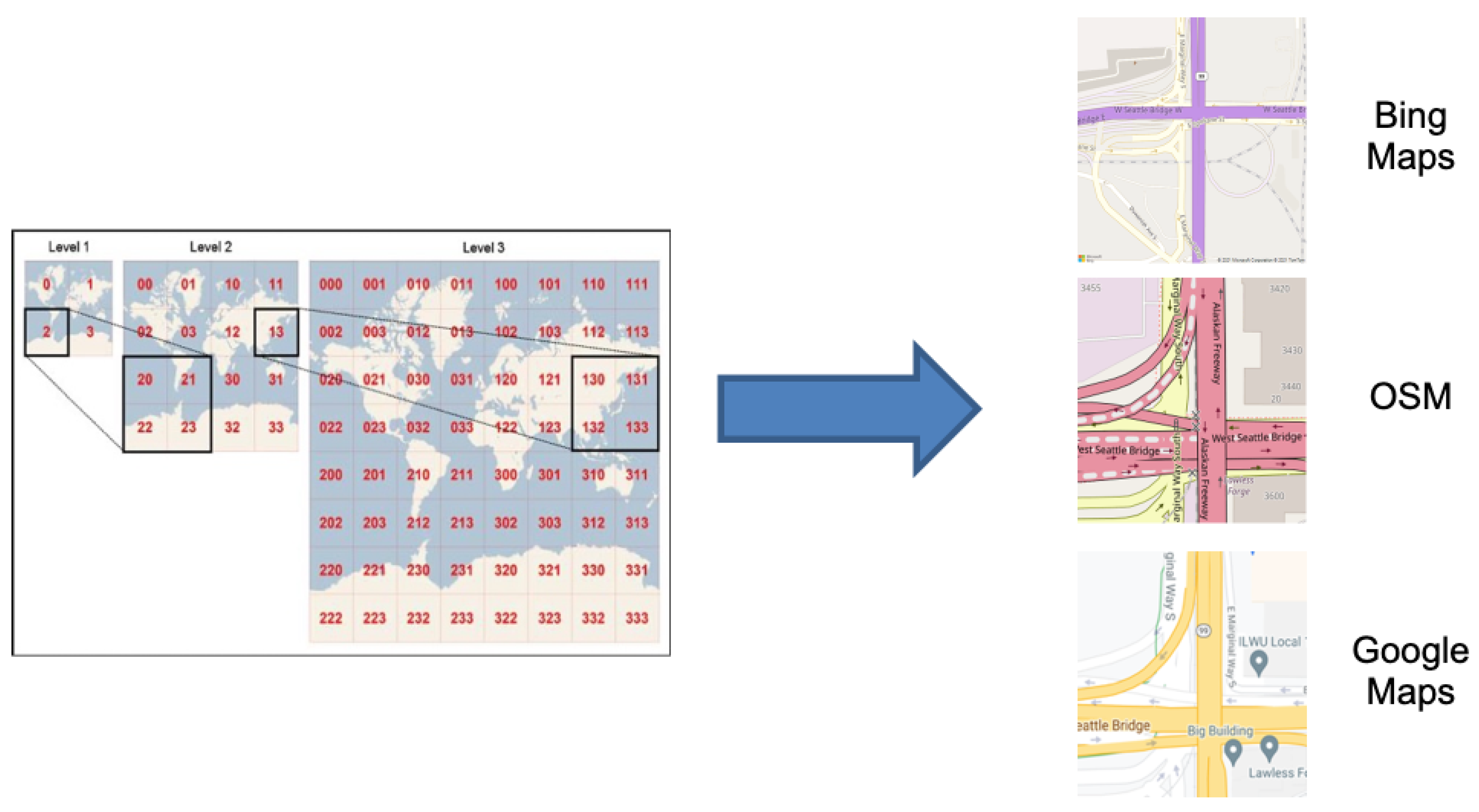
In this section, we present an architecture overview of the RDNN component (Road-Directionality Neural Network):

As shown in Figure 4, we collect training images from different providers. We use an online tool called CVAT [29] to create a labeled training dataset in COCO format. The labeling is performed manually. We use the training dataset to retrain an existing model from the Detectron2 model zoo. Essentially, we are starting with pre-trained model weights, freeze all layers in the network, and retrain the last layer on our new training dataset. This mechanism provides us the advantage of reusing and utilizing all the high-level features and abstractions learned by the original network on huge amount of training datasets. These same high-level features and abstractions are usually still useful for general object detection even for new classes. This allows us to obtain really good accuracy for detecting arrows while using a small amount of training dataset. This is extremely important because there is no existing online training dataset for arrows, and creating them manually is very time-consuming. Thus, reducing the amount of training dataset needed is extremely valuable.

2.3. Data Gathering

To obtain training data, we use APIs provided by different providers to download images for certain locations at specific zoom level. Under the cover, map providers use a Tile Map System [30] to be able to provide map image collections at different zoom levels. This system divides a large map into four quarters and then recursively divides each quarter into 4 quarters as the zoom level increases. Figure 5 shows an example of the Bing Maps Tile System.

We utilize the API provided by map providers to collect images for regions of interest at different zoom levels. Arrows only appear at high zoom levels. In this paper, we use zoom level 18 which we note to be the most suitable zoom level for analyzing road directionality.

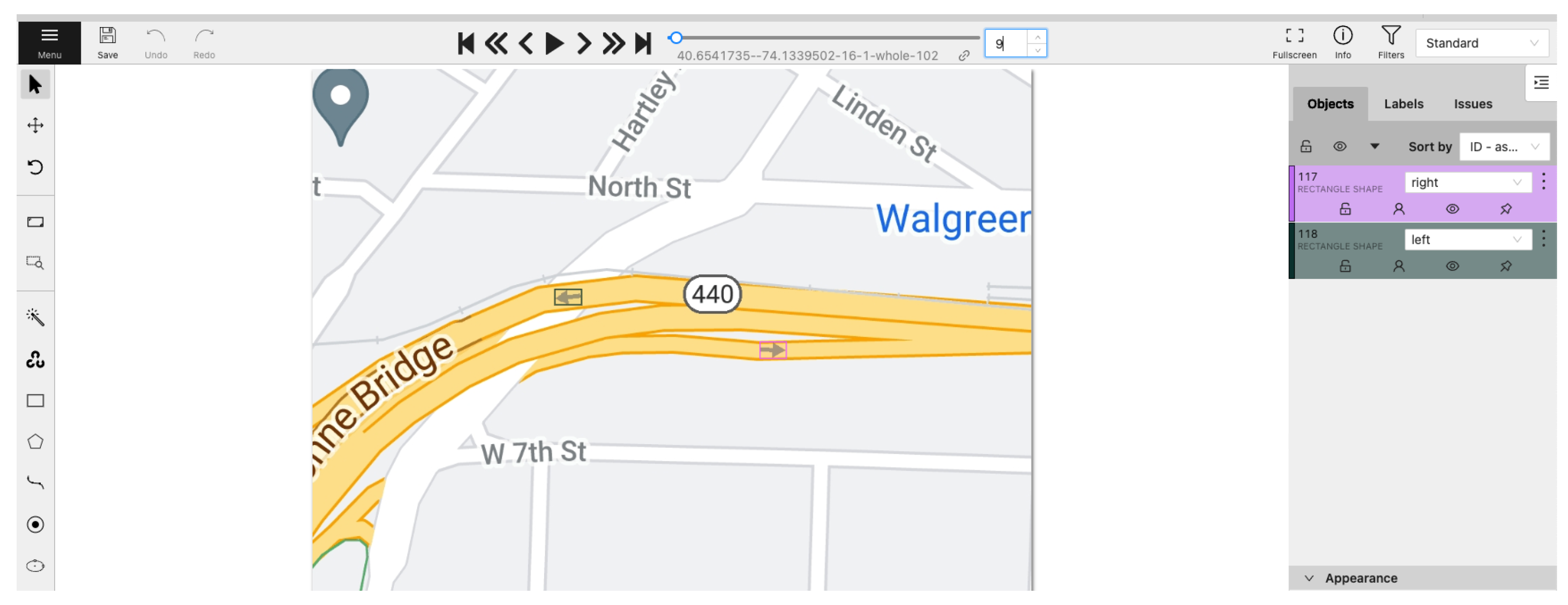
2.4. Data Preparation and Labelling

We need to train our neural network to detect the new classes related to arrow directionality. However, there is no such training data available online. Thus, we prepare our own training and test datasets. We use an online labeling tool called CVAT. As can be seen in Figure 6, this tool allows us to draw polygons and bounding boxes around objects of interest and label them.

We perform the labeling manually by identifying each arrow that appears in the image and drawing a box around it. We prepare and label many images for each provider. We then use the tool to generate this training dataset in COCO format. We similarly label another set of images to be used as the test dataset. This test dataset becomes the ground truth that we use to measure the accuracy of the model. We contribute both the training and test datasets and make them available online to be utilized by any future work in this area. The training dataset can be used to train similar neural networks for detecting arrow directionality in map images. The test datasests can be used as a baseline benchmark.

2.5. Hardware Requirements

Detectron2 neural networks use PyTorch GPU for training. Thus, we run all our experiments on the Google COLAB platform which provides a cloud infrastructure and resources with GPU capabilities.

3. Results and Discussion

We conduct several different experiments throughout this paper. In this section, we share the results for each experiment.

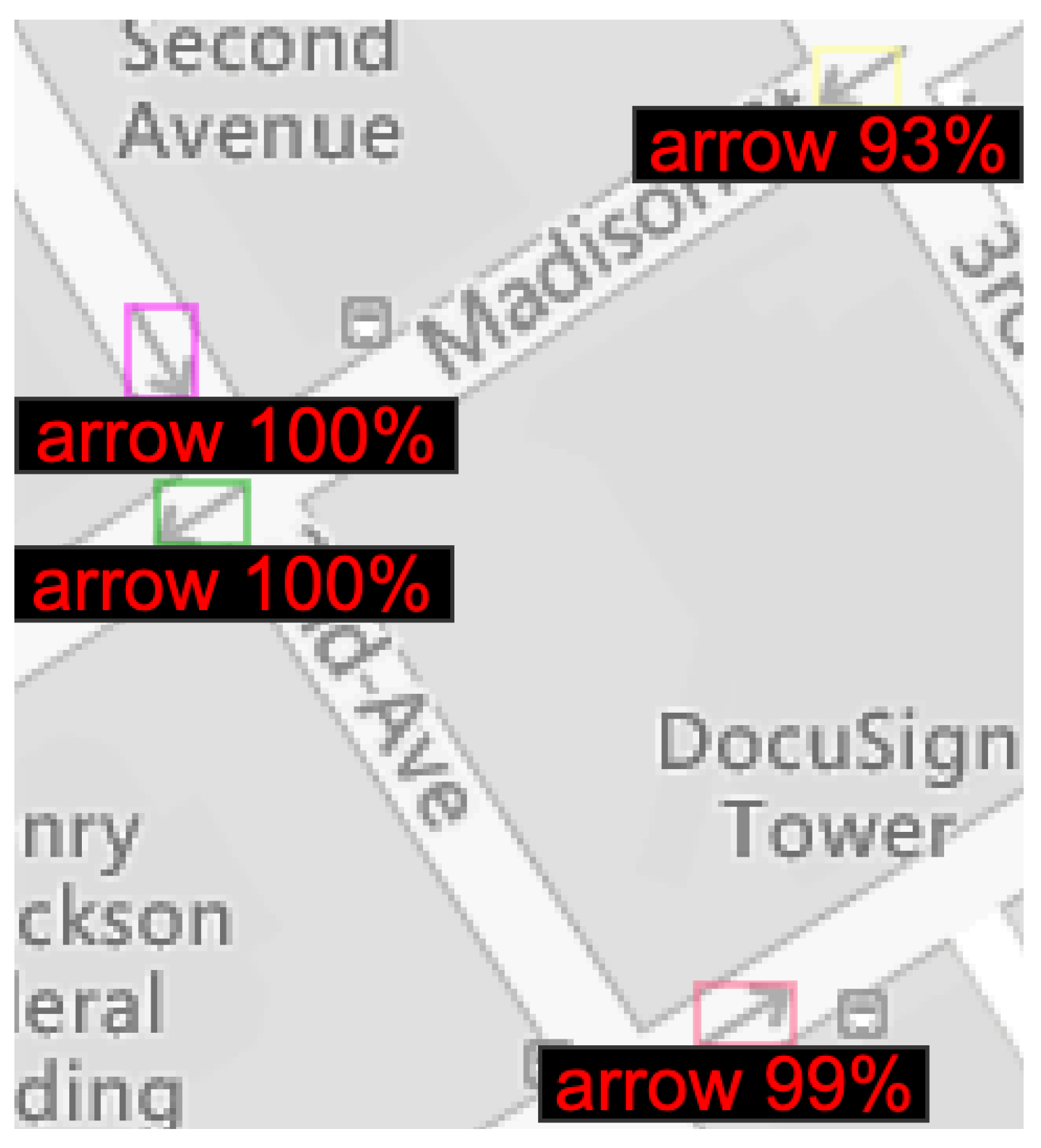
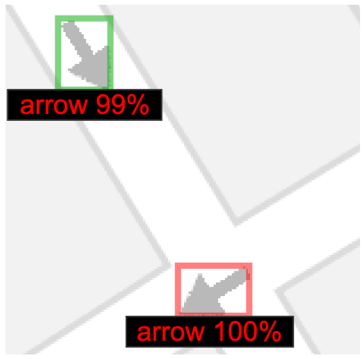
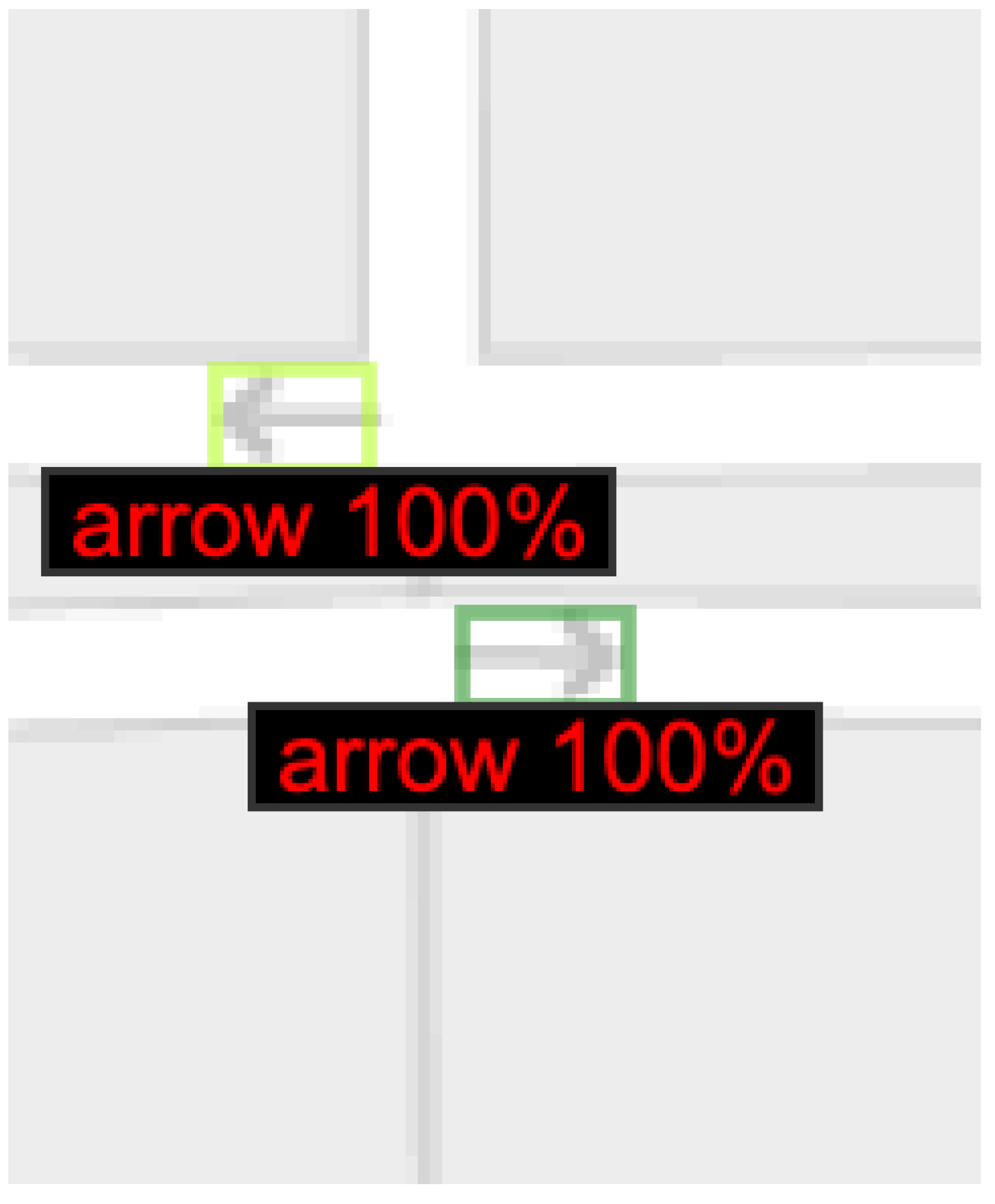
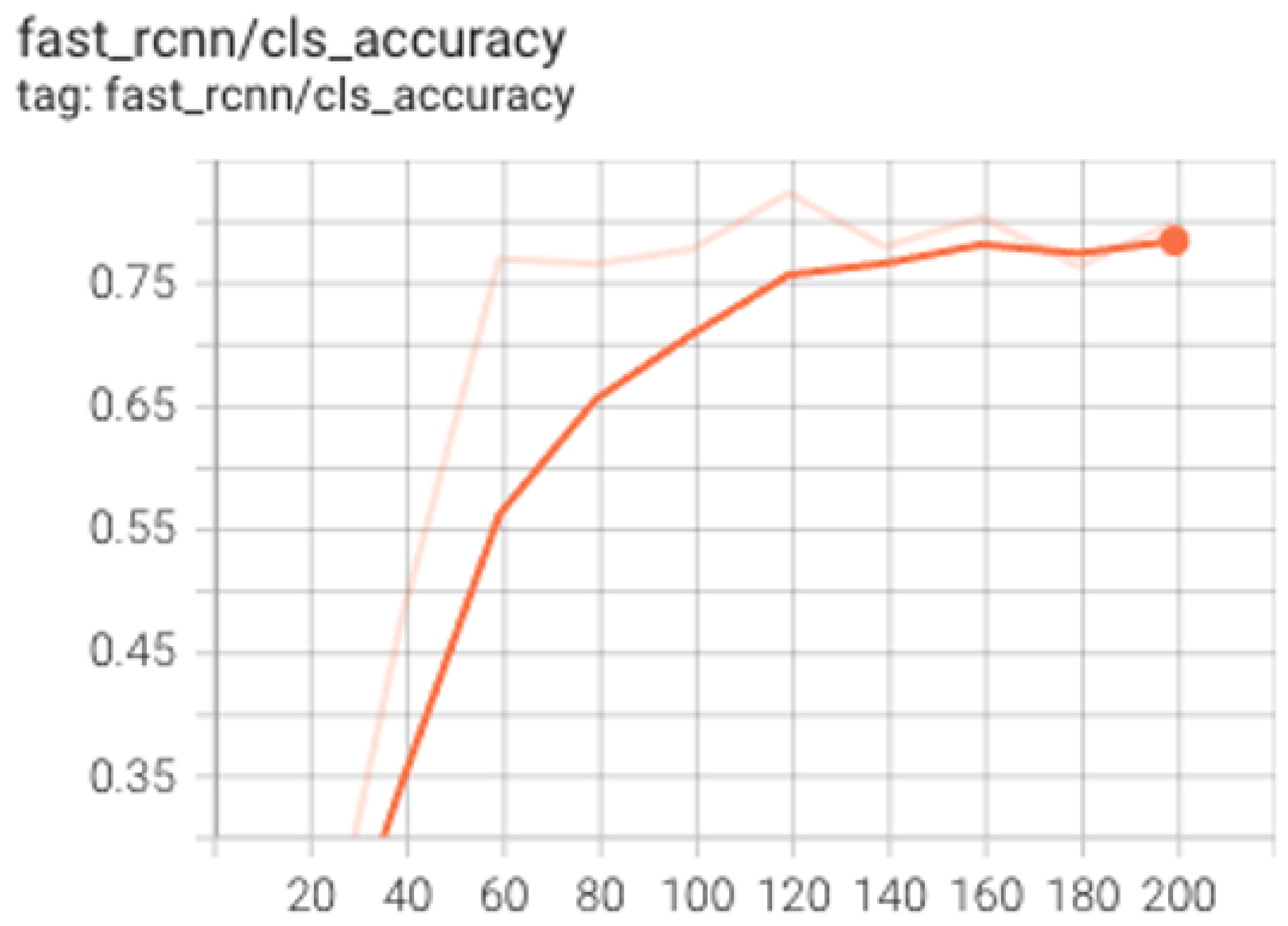
3.1. Experiment #1: Arrow Detection

In this experiment, we focus on detecting arrow objects in all the map providers: Bing Maps, Google Maps, and OSM. The challenge is that each provider uses a different style and size for arrows. Furthermore, even a single provider such as Bing Maps uses many different arrow styles for different road types. Google Maps is the easiest to work with because the arrow figure in the map is relatively thick and large. On the other hand, Bing Maps and OSM use arrow figures that are much skinnier and smaller which make them harder to detect. All the above make arrows detection harder for Bing Maps and OSM.

There are two main approaches to go about this. One is to build different models and train them separately for each provider. The other is to use one model and train it on training datasets containing images from all providers. To avoid the complexity of managing multiple models and to create a more general solution, we choose to go with the approach of one model hoping that the network will learn some deep underlying feature of what really makes an arrow figure and generalize over the superficial differences of style, color, and size of the arrow. We prepare a total of 296 training data points across all providers, and we train the network on this data. After tuning the network, we achieve the following rates:

As seen in

Table 2. Experiment #1—performance summary.

Provider:	Google Maps	Bing Maps	OSM
AP50	97.9%	88.7%	99.6%
AR50	100%	90.1%	100%
F1 Score	98.9%	89.3%	99.8%

above, we achieve a very high F1-Score for Google Maps and OSM. Bing Maps’ F1-Score is 89.3%. This is due to the challenging small profiles for Bing Maps arrows and the use of many different styles and profiles of arrows for different road types. We believe this can be improved using more training datasets covering the different arrow profiles. We address this implicitly in the next experiment where we shift our focus to detect arrow directionality, and as part of that, we prepare a much larger training dataset.

We use the model to perform inference on sample images to visualize the quality of the results. Figure 7, Figure 8, Figure 9 and Figure 10 present sample outputs of the model, which demonstrate its efficacy:

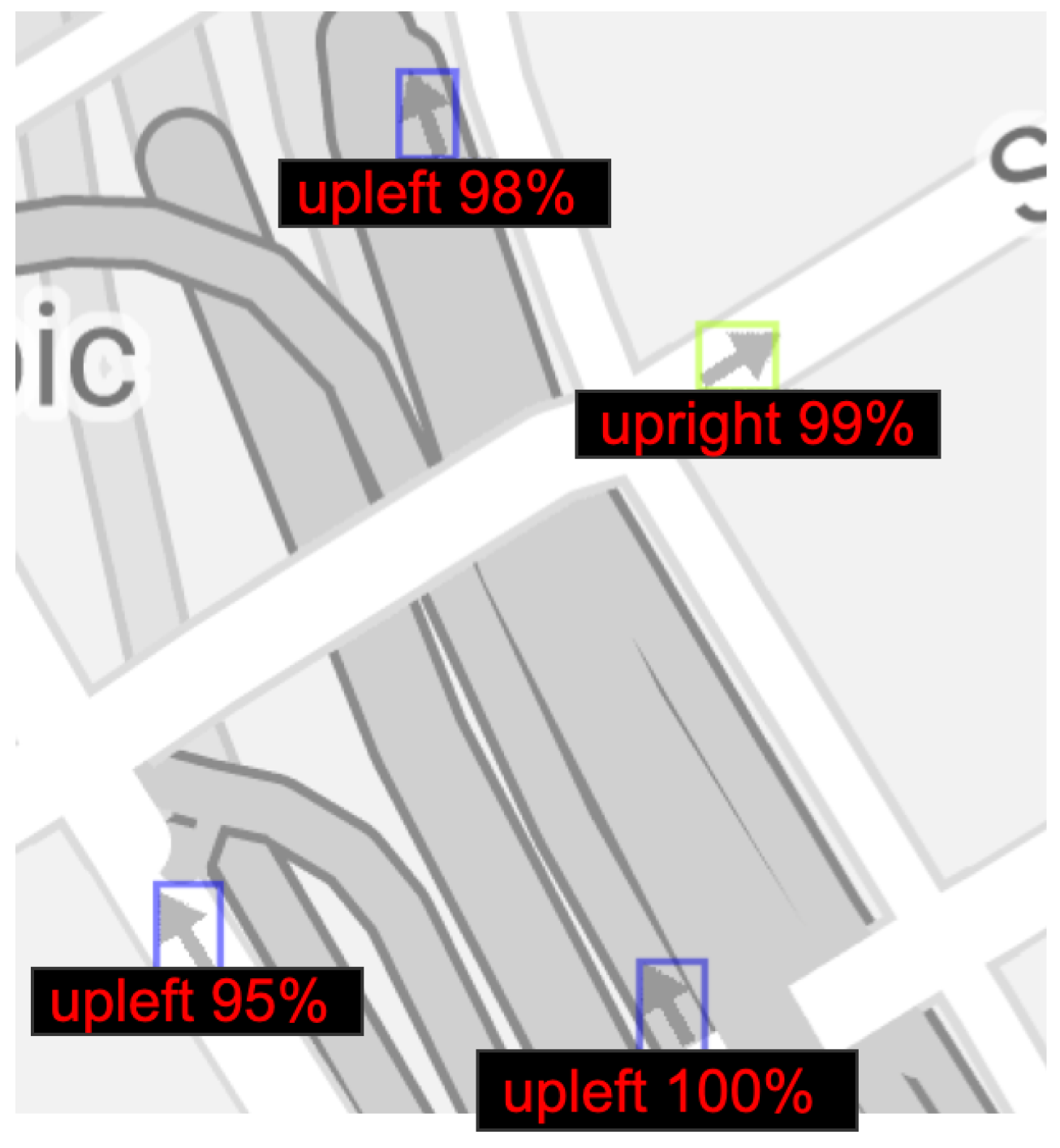
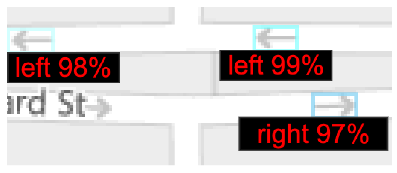
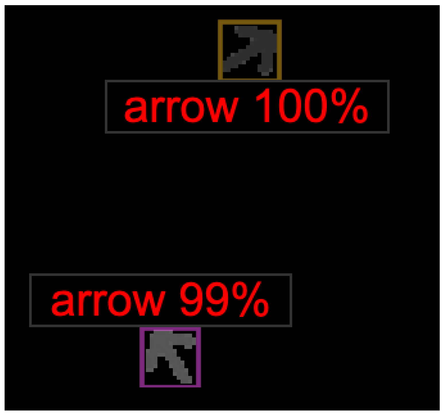
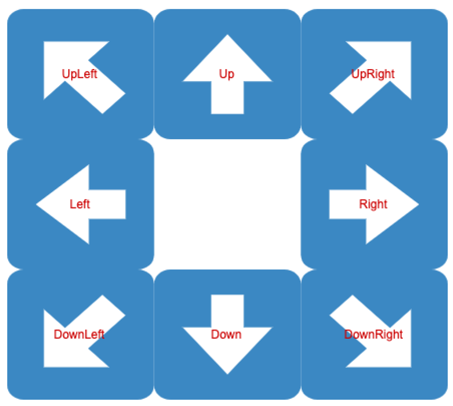
3.2. Experiment #2: Arrow Directionality Detection

One of the main goals of this research is to also detect arrow directionality. In this experiment, we change the previous model and extend it to detect arrow direction as well. We use a similar training dataset as previous experiments; however, we use different labels to indicate arrow direction. More specifically, we use eight cardinal directions to approximate arrow directionality as right, left, up, down, up-right, up-left, down-right, and down-left. Figure 11 shows the directions. These eight cardinal directions are enough for our purpose to determine the road direction.

Determining arrow directionality is a much harder task. Thus we prepare a much larger training dataset containing 2493 data points covering all data providers and all eight cardinal directions. We also use a deeper neural network and a faster_rcnn_101_FPN which has 101 layers compared to the network of 50 layers used in the previous experiment. We utilize this network because using the 50-layer network was not enough to capture the complexity of the training data and was not able to reduce the training dataset loss to an acceptable level. Figure 12 shows how our model’s accuracy plateaued at around 76% and failed to improve further when using only 50 layers.

We also turn off the automatic image rotation which is part of standard data augmentation performed by the model. This is because our labels are sensitive to directions, and rotating the images will result in incorrect labels.

We train our model and fine-tune the neural network to find the best results.

Table 3. Experiment #2—performance summary.

Provider:	Google Maps	Bing Maps	OSM
AP50	91.8%	90.7%	95.3%
AR50	92.1%	91.3%	95.8%
F1 Score	91.9%	91.0%	95.5%

presents the precision and recall rates that our model has achieved. As shown in this table, our model achieves > 90% precision and recall on detecting arrow directionality for all providers.

We use the model to perform inference on sample images to visualize the quality of the results. Figure 13, Figure 14 and Figure 15 present sample outputs of our proposed model. As can be seen in Figure 13, Figure 14 and Figure 15, our model is able to successfully create bounding boxes for the arrows’ positions and identify their directionality. The percentages indicate how confident our model is in its assessment. The arrows in Figure 13 show that the model correctly distinguishes between the arrows oriented up-left and the arrows oriented up-right. Similarly, our model is capable of identifying the arrows within the image that is shown in Figure 14 as left and right orientations although the arrow profile is extremely small. Furthermore, Figure 15 shows that our model can detect arrows with the correct orientation on OSM which has a significantly different background compared to those in Figure 13 and Figure 14.

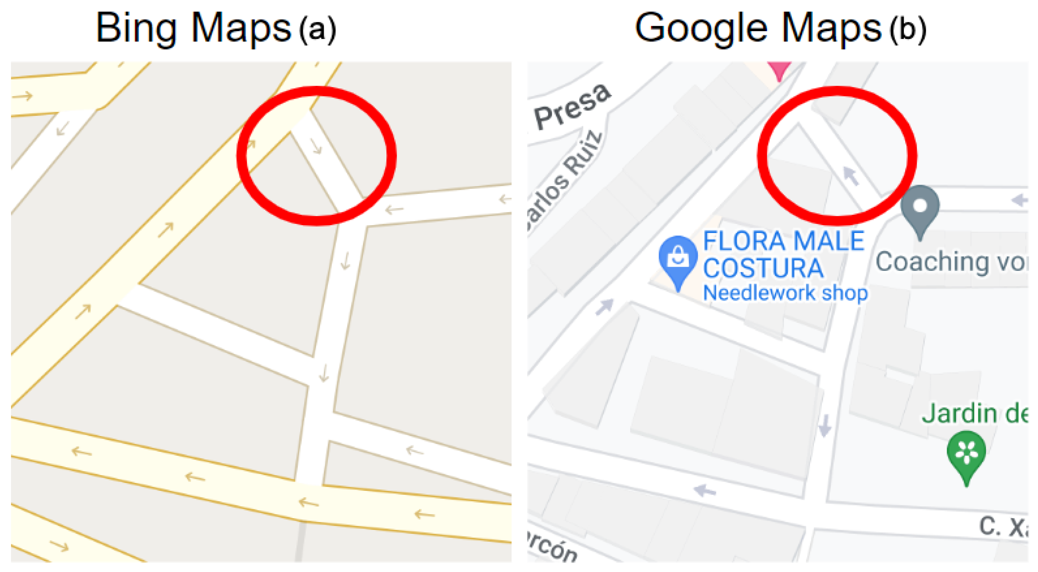
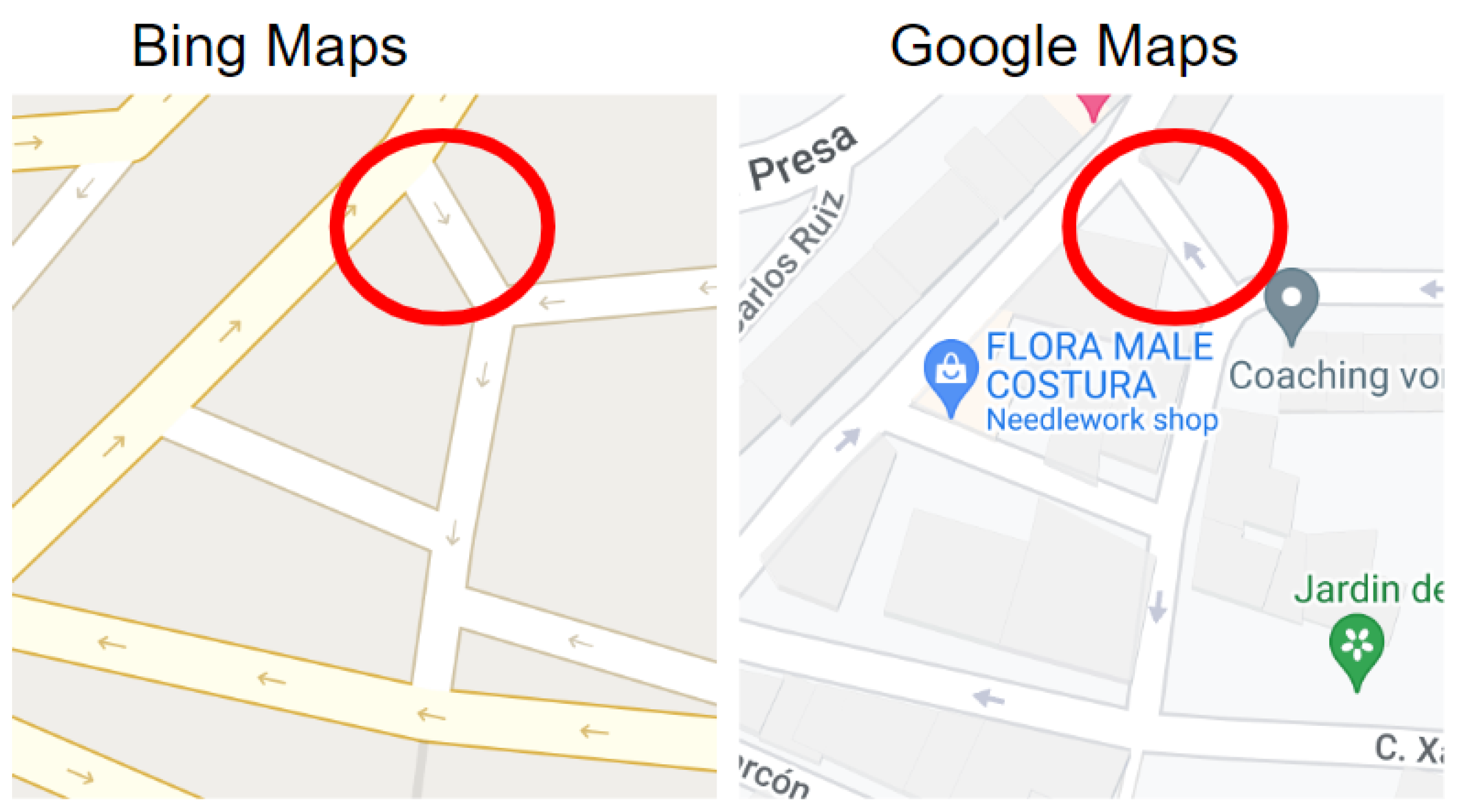
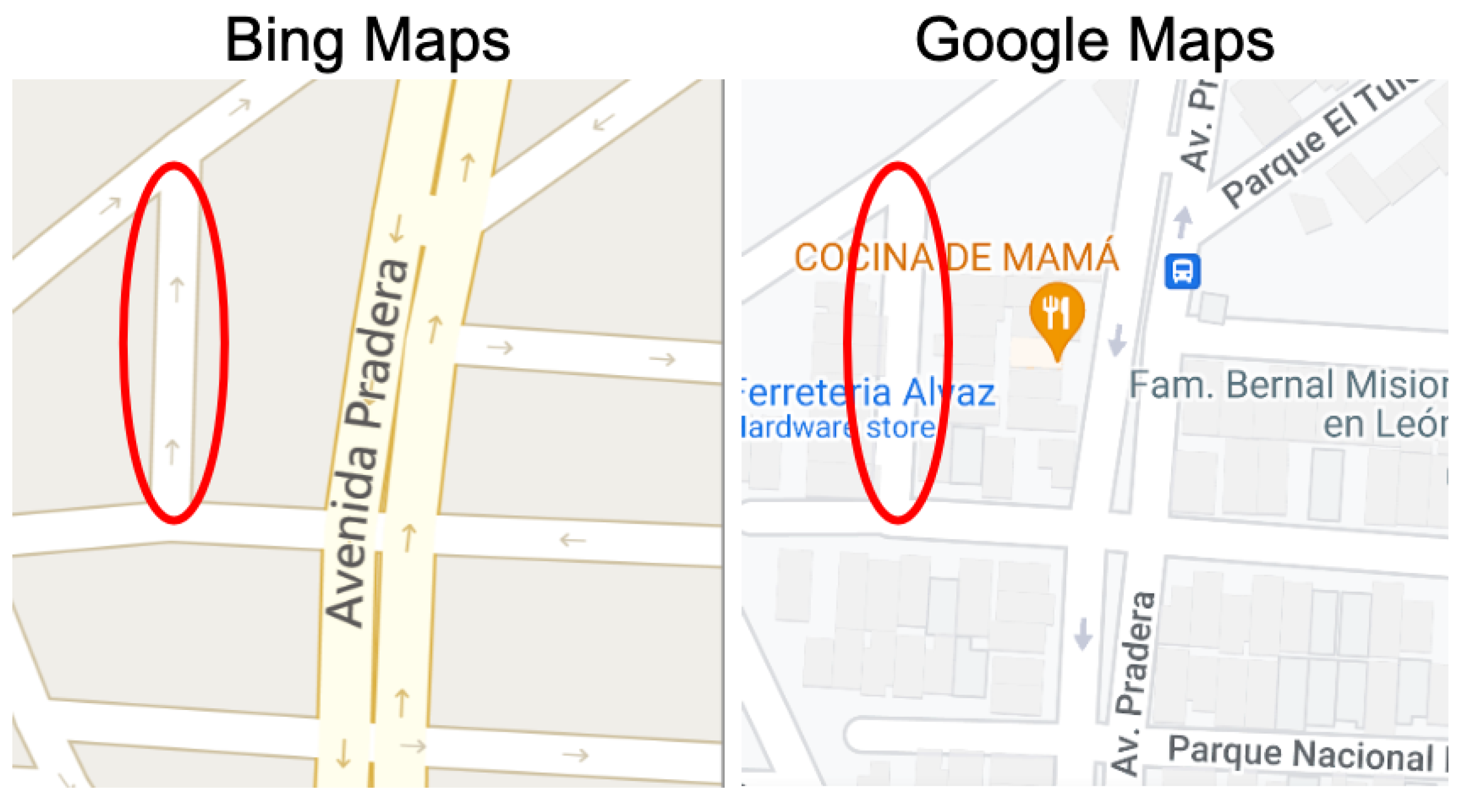
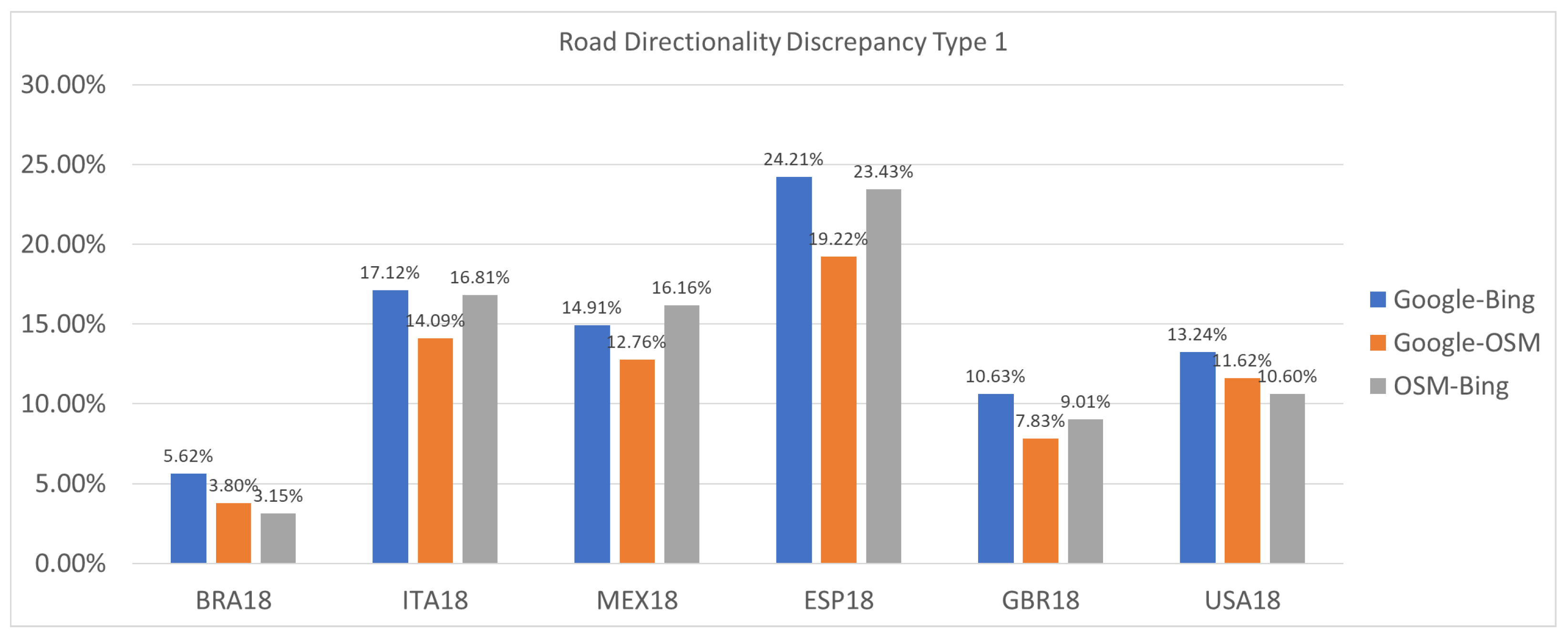
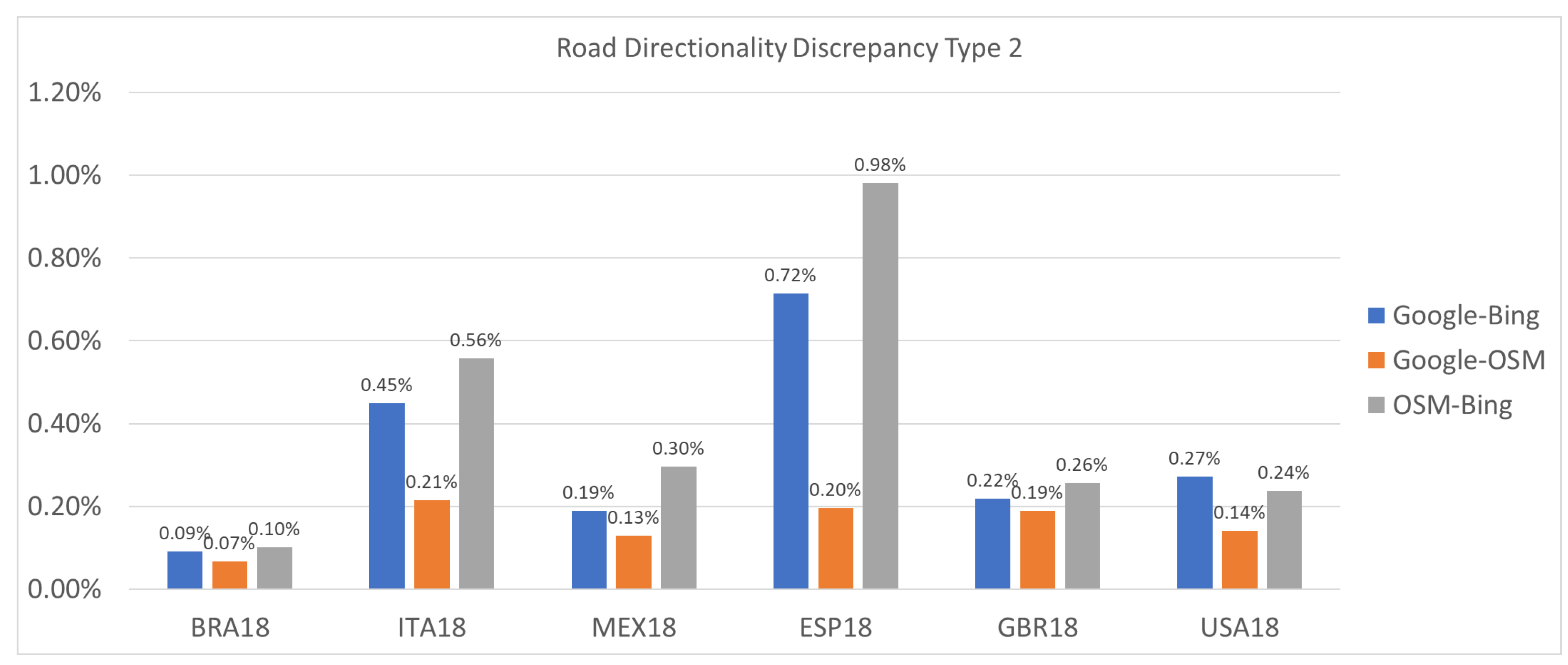
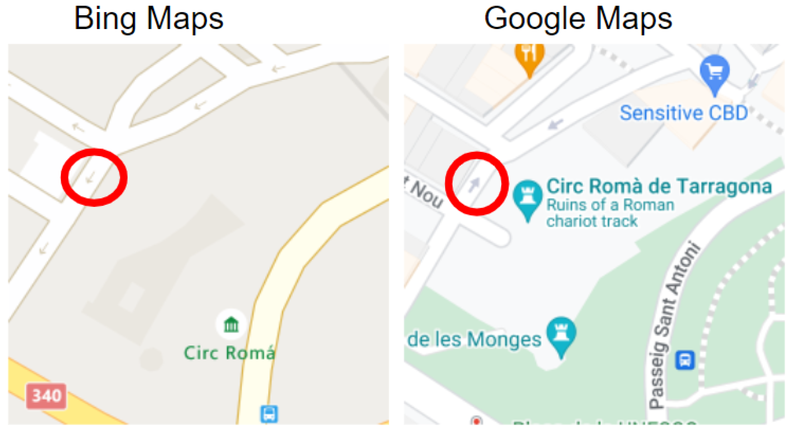
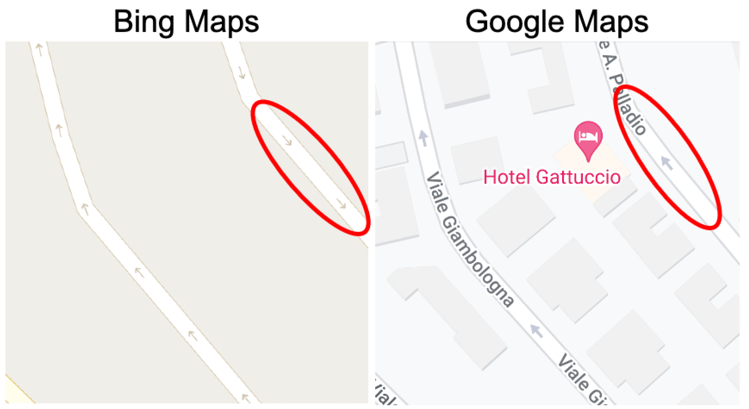
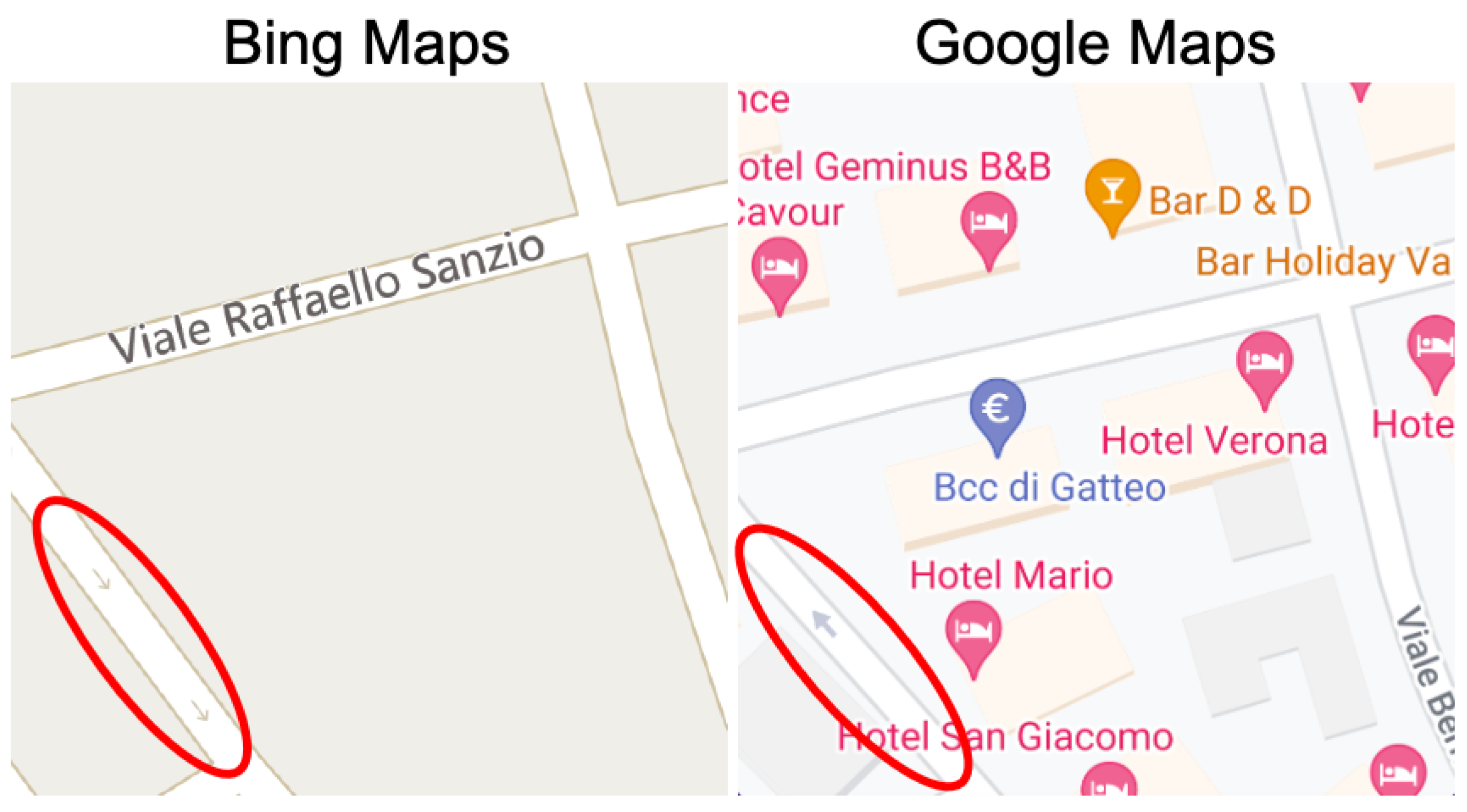
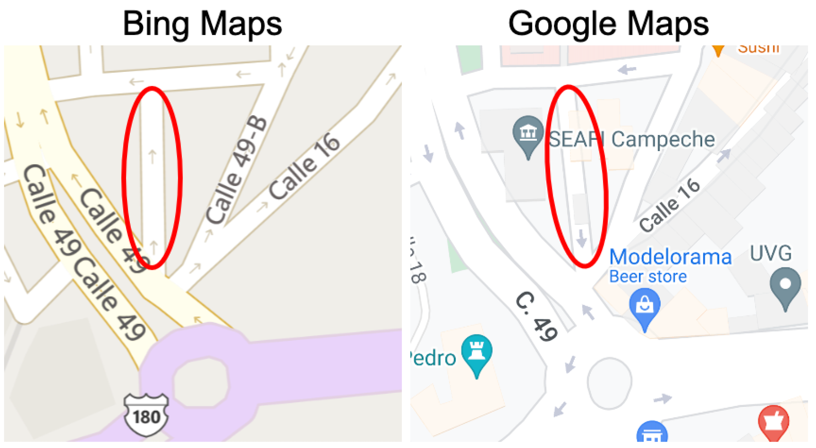
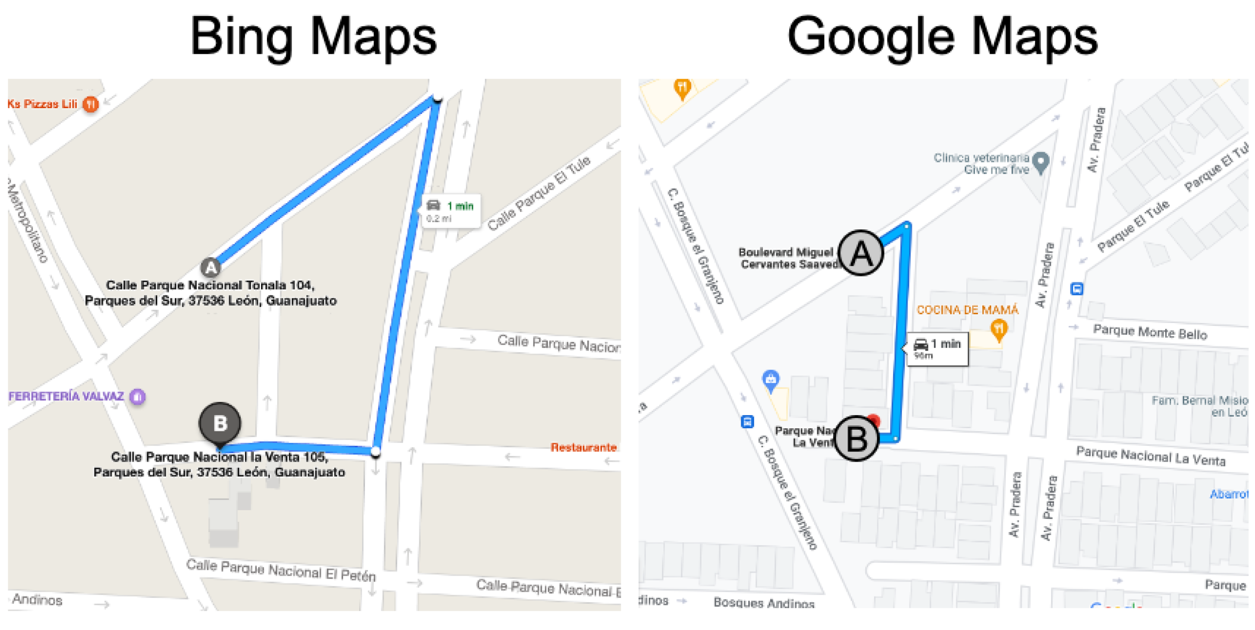
3.3. Experiment #3: Detecting Discrepancies in Road Directions across Map Providers

In this experiment, we combine and analyze the results of two components. First, we use the road directionality neural network (RDNN) to extract arrow directionality. Second, we use a binarization-based component developed by University of Washington researchers [5] which produces a binary and skeleton representation of the roads in a given map image. We utilize both components to detect discrepancies across map providers. Figure 16 helps illustrate how we perform comparisons. We define road segments as road stretches between intersections and then overlay the segments with the arrow directionality information detected from our model. We note that every road segment might contain many arrows due to reasons such as multiple arrows being placed on the road or the road being bi-directional. Thus, we keep track of a set of arrows for every road segment. The comparison is performed based on the set of different arrow directions that exist in the corresponding road segment rather than just the count of arrows. We then match each road segment across different providers based on map locality and scan for discrepancies in arrow direction. Two map images will not typically be able to match all road segments since some roads might be displayed by only one provider. For this reason, our model only compares the directions for road segments that exist in both images.

We investigate thousands of map images corresponding to coordinates randomly selected from six regions: Spain, Great Britain, the United States, Italy, Brazil, and Mexico. We define two types of discrepancies:

• Type 1 (Weak Discrepancy): This is defined when one provider has arrows indicating a specific direction for a road segement while the other provider is missing any arrows info for the same road segment;
• Type 2 (Strong Discrepancy): This occurs when both providers have arrows for a road segment but their directions do not match, indicating a conflicting road direction.

Both types of discrepancies are of interest and value, but Type 2 discrepancies are our primary concern due to the severity of the error that must occur in a map to generate such discrepancies. Moreover, they present serious safety hazards due to potentially causing drivers to drive in the wrong direction. These discrepancies are far rarer, occurring in fewer than 1% of the road directions compared. This is to be expected given that map providers take great care to avoid displaying incorrect road directions.

Type 1 is also of great value because first it indicates lack of essential map info for some of the areas, but also, by default, the lack of directions is usually an indication that the map provider is treating this road as bi-directional which also could lead to a safety hazard.

Figure 17 and Figure 18 show the percentages of each type of discrepancy found in a given region.

For example, for Spain, our Google Maps vs. Bing Maps comparison detects strong discrepancies representing a percentage of 0.72%. Figure 19 and Figure 20 present strong discrepancies examples found in this region for Google Maps vs. Bing Maps.

Similarly, our system detects strong discrepancies of 0.45% in Italy and 0.19% in Mexico for the Google Maps vs. Bing Maps comparison. Figure 21, Figure 22 and Figure 23 show some examples.

Due to their rarity and the importance of identifying such discrepancies, our system errs on the side of caution, reporting anything that might be a Type 2 discrepancy. Some of these are false positives, but false positives are preferable to false negatives. Though not all Type 2 discrepancies reported are guaranteed to correspond to genuine errors, our system can help dramatically narrow down the locations that need to be searched through. Our system reports the discrepancy count for each coordinate to help facilitate this manual investigation.

For example,

Table 4. Type 2 Discrepancy precision metrics in Spain.

Comparison	Total Discrepancies Reported	True Positives	Precision
Google Maps vs. Bing Maps	4	3	75%
Google Maps vs. OSM	1	0	0%
Bing Maps vs. OSM	8	3	37.5%

represents the precision of strong discrepancies reported by our system in Spain.

Type 1 (Weak Discrepancy) is also of great value because first it indicates lack of essential map information for some of the areas, but also the lack of direction information usually indicates the map provider is considering this road bi-directional which is the default. This also can lead to a serious safety hazard. For example let us consider the following weak discrepancy found by our system in Mexico:

In Figure 24 above, Bing Maps has an arrow pointing north for the road circled with red, indicating the road segment is one direction. However, Google does not have any arrow for this road segment which suggests the road is bi-directional by default. To validate this, we investigate the routes provided by both providers. Figure 25 presents the routes from point A to point B in both maps.

Google clearly uses this road in the opposite direction (going south), while Bing avoids this road and chooses an alternate longer route. We investigate the satellite images for this road and use it as a ground truth, which seem to indicate the road is indeed one-directional going north. This is a clear example where a weak discrepancy uncovers a scenario where a provider is utilizing a road in the wrong direction, posing serious safety hazards.

4. Conclusions

In this paper, we investigated the challenge of detecting an arrow’s location and directionality in map images across different providers. We presented a neural network model that detected the arrow directionality with more than 90% F1-Score for the different providers (Google Maps: 91.9%, Bing Maps: 91.0%, OSM: 95.5%). We then utilized the model, along with a road segment detection component, to automatically analyze and scan randomly chosen study areas and reported percentage of discrepancies discovered in road directions for the different study areas. We also compiled a list of these discrepancies for further manual investigation. Our system uncovered real examples of conflicting road directions across map providers, proving such discrepancies do exist and pose serious safety hazards. Such an experiment shows the usability of our system to scan large map areas and automatically detect and report matches and discrepancies to help guide the next efforts of error corrections and quality improvements of maps in certain areas.

References

1. 9 Things to Know about Google’s Maps Data: Beyond the Map. Available online: https://cloud.google.com/blog/products/maps-platform/9-things-know-about-googles-maps-data-beyond-map (accessed on 4 April 2022).
2. Ciepluch, B.; Jacob, R.; Mooney, P.; Winstanley, A.C. Comparison of the accuracy of OpenStreetMap for Ireland with Google Maps and Bing Maps. In Proceedings of the Ninth International Symposium on Spatial Accuracy Assessment in Natural Resuorces and Enviromental Sciences, Leicester, UK, 20–23 July 2010; p. 337. [Google Scholar]
3. Bandil, A.; Girdhar, V.; Chau, H.; Ali, M.; Hendawi, A.; Govind, H.; Cao, P.; Song, A. GeoDart: A System for Discovering Maps Discrepancies. In Proceedings of the 2021 IEEE 37th International Conference on Data Engineering (ICDE), Chania, Greece, 19–22 April 2021; pp. 2535–2546. [Google Scholar] [CrossRef]
4. Basiri, A.; Jackson, M.; Amirian, P.; Pourabdollah, A.; Sester, M.; Winstanley, A.; Moore, T.; Zhang, L. Quality assessment of OpenStreetMap data using trajectory mining. Geo-Spat. Inf. Sci. 2016, 19, 56–68. [Google Scholar] [CrossRef]
5. A Geospatial Method for Detecting Map-Based Road Segment Discrepancies. Available online: http://faculty.washington.edu/mhali/Publications/Publications.htm (accessed on 10 March 2021).
6. Bandil, A.; Girdhar, V.; Dincer, K.; Govind, H.; Cao, P.; Song, A.; Ali, M. An interactive system to compare, explore and identify discrepancies across map providers. In Proceedings of the 28th International Conference on Advances in Geographic Information Systems, Seattle, WA, USA, 3–6 November 2020; pp. 425–428. [Google Scholar]
7. Unsalan, C.; Sirmacek, B. Road Network Detection Using Probabilistic and Graph Theoretical Methods. IEEE Trans. Geosci. Remote Sens. 2012, 50, 4441–4453. [Google Scholar] [CrossRef]
8. John, V.; Zheming, L.; Mita, S. Robust traffic light and arrow detection using optimal camera parameters and GPS-based priors. In Proceedings of the 2016 Asia-Pacific Conference on Intelligent Robot Systems (ACIRS), Tokyo, Japan, 20–22 July 2016; pp. 204–208. [Google Scholar] [CrossRef]
9. Santosh, K.C.; Wendling, L.; Antani, S.; Thoma, G.R. Overlaid Arrow Detection for Labeling Regions of Interest in Biomedical Images. IEEE Intell. Syst. 2016, 31, 66–75. [Google Scholar] [CrossRef]
10. Schäfer, B.; Keuper, M.; Stuckenschmidt, H. Arrow R-CNN for handwritten diagram recognition. Int. J. Doc. Anal. Recognit. (IJDAR) 2021, 24, 3–17. [Google Scholar] [CrossRef]
11. Girshick, R. Fast r-cnn. In Proceedings of the IEEE International Conference on Computer Vision, Santiago, Chile, 7–13 December 2015; pp. 1440–1448. [Google Scholar]
12. Ren, S.; He, K.; Girshick, R.; Sun, J. Faster r-cnn: Towards real-time object detection with region proposal networks. Adv. Neural Inf. Process. Syst. 2015, 28, 91–99. [Google Scholar] [CrossRef]
13. Wu, Y.; Kirillov, A.; Massa, F.; Lo, W.-Y.; Girshick, R. Detectron2. 2019. Available online: https://github.com/facebookresearch/detectron2 (accessed on 17 May 2022).
14. Dosovitskiy, A.; Beyer, L.; Kolesnikov, A.; Weissenborn, D.; Zhai, X.; Unterthiner, T.; Dehghani, M.; Minderer, M.; Heigold, G.; Gelly, S.; et al. An image is worth 16x16 words: Transformers for image recognition at scale. arXiv 2020, arXiv:2010.11929. [Google Scholar]
15. Liu, Z.; Lin, Y.; Cao, Y.; Hu, H.; Wei, Y.; Zhang, Z.; Lin, S.; Guo, B. Swin transformer: Hierarchical vision transformer using shifted windows. In Proceedings of the IEEE/CVF International Conference on Computer Vision, Montreal, QC, Canada, 10–17 October 2021; pp. 10012–10022. [Google Scholar]
16. Liu, Z.; Mao, H.; Wu, C.Y.; Feichtenhofer, C.; Darrell, T.; Xie, S. A convnet for the 2020s. In Proceedings of the IEEE/CVF Conference on Computer Vision and Pattern Recognition, New Orleans, LA, USA, 19–20 June 2022; pp. 11976–11986. [Google Scholar]
17. Yu, T.; Huang, H.; Jiang, N.; Acharya, T.D. Study on Relative Accuracy and Verification Method of High-Definition Maps for Autonomous Driving. ISPRS Int. J. Geo-Inf. 2021, 10, 761. [Google Scholar] [CrossRef]
18. Ma, J.; Sun, Q.; Zhou, Z.; Wen, B.; Li, S. A Multi-Scale Residential Areas Matching Method Considering Spatial Neighborhood Features. ISPRS Int. J. Geo-Inf. 2022, 11, 331. [Google Scholar] [CrossRef]
19. Alghanim, A.; Jilani, M.; Bertolotto, M.; McArdle, G. Leveraging Road Characteristics and Contributor Behaviour for Assessing Road Type Quality in OSM. ISPRS Int. J. Geo-Inf. 2021, 10, 436. [Google Scholar] [CrossRef]
20. Koukoletsos, T.; Haklay, M.; Ellul, C. An automated method to assess data completeness and positional accuracy of OpenStreetMap. In Proceedings of the GeoComputation, London, UK, 20–22 July 2011. [Google Scholar]
21. Brovelli, M.A.; Minghini, M.; Molinari, M.E. An Automated GRASS-Based Procedure to Assess the Geometrical Accuracy of the OpenStreetMap Paris Road Network. In Proceedings of the ISPRS Congress, Prague, Czech Republic, 12–19 July 2016. [Google Scholar]
22. Brovelli, M.A.; Minghini, M.; Molinari, M.; Mooney, P. Towards an automated comparison of OpenStreetMap with authoritative road datasets. Trans. GIS 2017, 21, 191–206. [Google Scholar] [CrossRef]
23. Jackson, S.P.; Mullen, W.; Agouris, P.; Crooks, A.; Croitoru, A.; Stefanidis, A. Assessing completeness and spatial error of features in volunteered geographic information. ISPRS Int. J. Geo-Inf. 2013, 2, 507–530. [Google Scholar] [CrossRef]
24. Ludwig, I.; Voss, A.; Krause-Traudes, M. A Comparison of the Street Networks of Navteq and OSM in Germany. In Advancing Geoinformation Science for a Changing World; Springer: Berlin/Heidelberg, Germany, 2011; pp. 65–84. [Google Scholar]
25. Zielstra, D.; Hochmair, H.H. Using free and proprietary data to compare shortest-path lengths for effective pedestrian routing in street networks. Transp. Res. Rec. 2012, 2299, 41–47. [Google Scholar] [CrossRef]
26. Vokhidov, H.; Hong, H.G.; Kang, J.K.; Hoang, T.M.; Park, K.R. Recognition of Damaged Arrow-Road Markings by Visible Light Camera Sensor Based on Convolutional Neural Network. Sensors 2016, 16, 2160. [Google Scholar] [CrossRef] [PubMed]
27. Lin, T.Y.; Dollár, P.; Girshick, R.; He, K.; Hariharan, B.; Belongie, S. Feature pyramid networks for object detection. In Proceedings of the IEEE Conference on Computer Vision and Pattern Recognition, Honolulu, HI, USA, 21–26 July 2017; pp. 2117–2125. [Google Scholar]
28. Lin, T.-Y.; Maire, M.; Belongie, S.; Hays, J.; Perona, P.; Ramanan, D.; Dollár, P.; Zitnick, C.L. Microsoft coco: Common objects in context. In European Conference on Computer Vision; Springer: Cham, Switerland, 2014; pp. 740–755. [Google Scholar]
29. CVAT. Available online: https://cvat.org/ (accessed on 4 February 2022).
30. Bing Maps Tile System. Available online: https://docs.microsoft.com/en-us/bingmaps/articles/bing-maps-tile-system?redirectedfrom=MSDN (accessed on 5 March 2022).
Figure 1. Discrepancy example of road directionality across different providers: (a) Bing Maps shows this road in Spain heading southeast; (b) Google Maps, however, shows this same road heading northwest.
Ijgi 11 00448 g001
Figure 2. Faster R-CNN high level architecture.
Ijgi 11 00448 g002
Figure 3. Overall system architecture.
Ijgi 11 00448 g003
Figure 4. Arrow directionality detection neural network architecture.
Ijgi 11 00448 g004
Figure 5. Bing Maps Tile System [30].
Ijgi 11 00448 g005
Figure 6. Data labeling using CVAT online tool.
Ijgi 11 00448 g006
Figure 7. Arrow position detection for Google Maps.
Ijgi 11 00448 g007
Figure 8. Arrow position detection for Bing Maps.
Ijgi 11 00448 g008
Figure 9. Arrow position detection for OSM.
Ijgi 11 00448 g009
Figure 10. Second arrow position detection for Bing Maps.
Ijgi 11 00448 g010
Figure 11. Classes used to classify arrow direction.
Ijgi 11 00448 g011
Figure 12. Training accuracy capping at 76% for Faster-RCNN with 50 layers.
Ijgi 11 00448 g012
Figure 13. Arrow direction detection for Google Maps.
Ijgi 11 00448 g013
Figure 14. Arrow direction detection for Bing Maps.
Ijgi 11 00448 g014
Figure 15. Arrow direction detection for OSM.
Ijgi 11 00448 g015
Figure 16. Road network generation architecture.
Ijgi 11 00448 g016
Figure 17. Road direction discrepancy stats Type 1 (weak discrepancy).
Ijgi 11 00448 g017
Figure 18. Road direction discrepancy stats Type 2 (strong discrepancy).
Ijgi 11 00448 g018
Figure 19. Type 2 (strong discrepancy) example #1-Spain.
Ijgi 11 00448 g019
Figure 20. Type 2 (strong discrepancy) example #2-Spain.
Ijgi 11 00448 g020
Figure 21. Type 2 (strong discrepancy) example #3-Italy.
Ijgi 11 00448 g021
Figure 22. Type 2 (strong discrepancy) example #4-Italy.
Ijgi 11 00448 g022
Figure 23. Type 2 (strong discrepancy) example #5-Mexico.
Ijgi 11 00448 g023
Figure 24. Type 1 (weak discrepancy) example-Mexico.
Ijgi 11 00448 g024
Figure 25. Discrepancy in route data—Mexico.
Ijgi 11 00448 g025