
Vegetation Greenness Trend in Dry Seasons and Its Responses to Temperature and Precipitation in Mara River Basin, Africa


 ,
, 
Abstract
:1. Introduction
2. The Study Area and Data
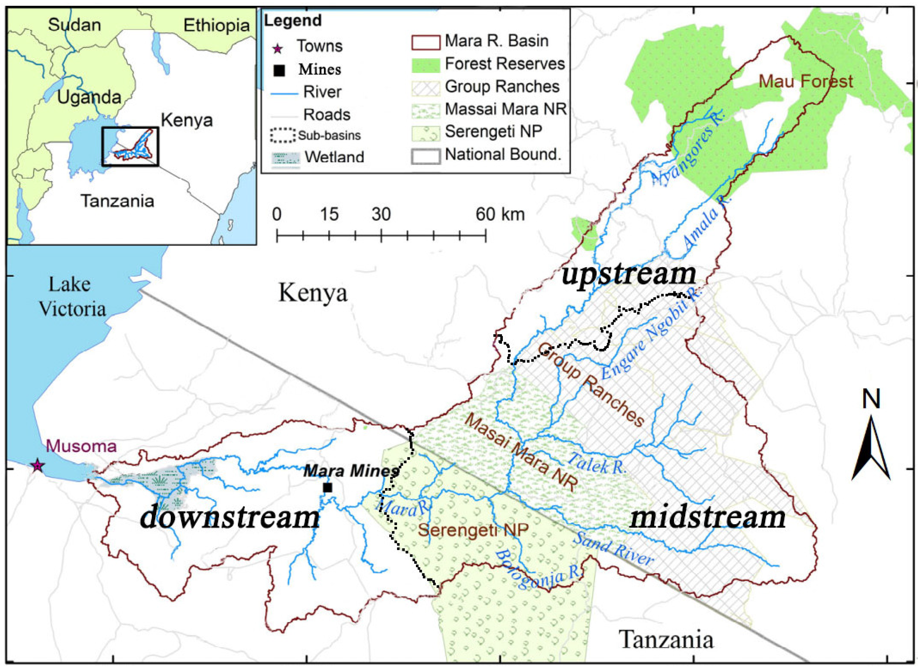
2.1. The Study Area
2.2. Data
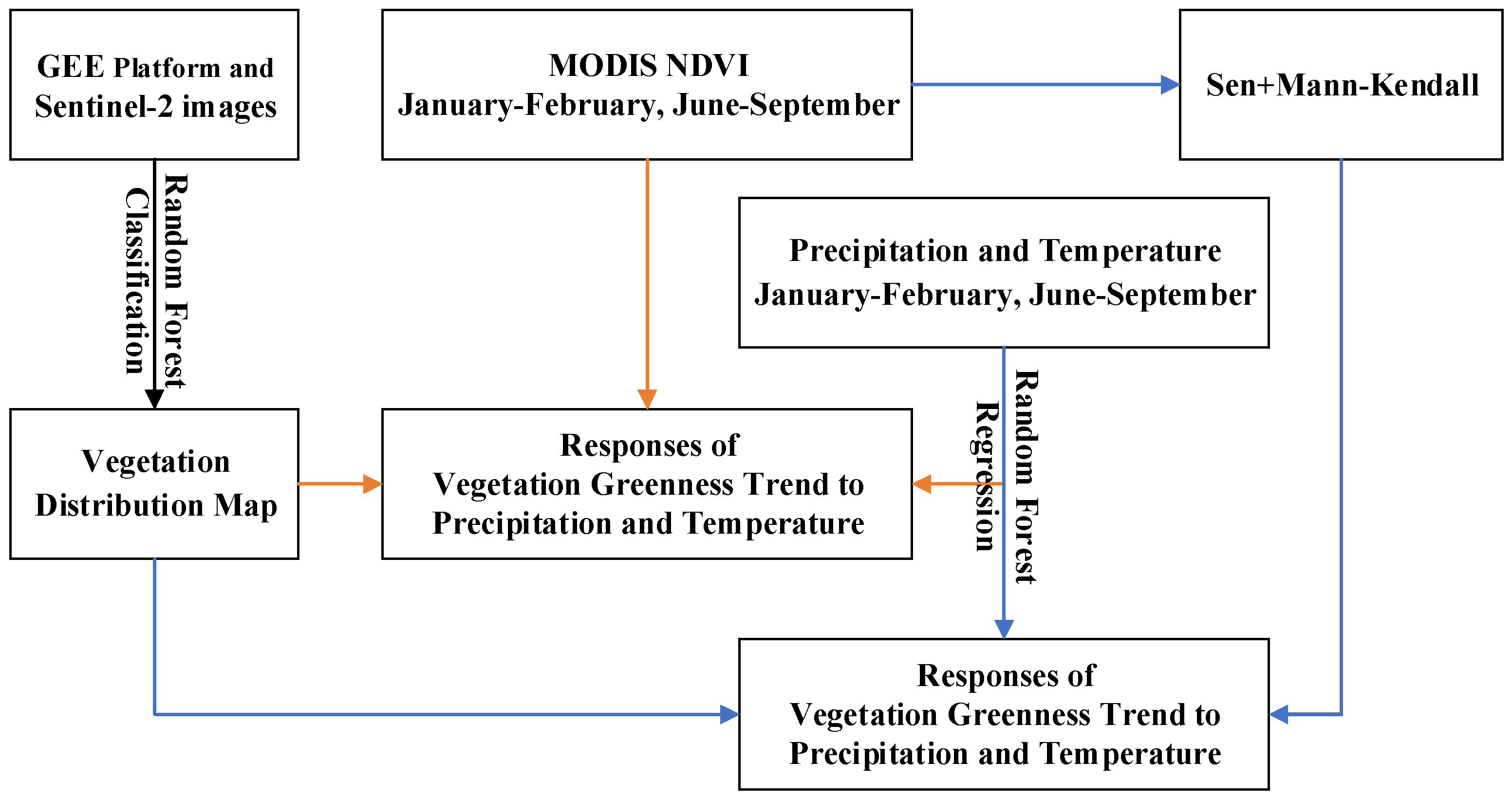
3. Methods
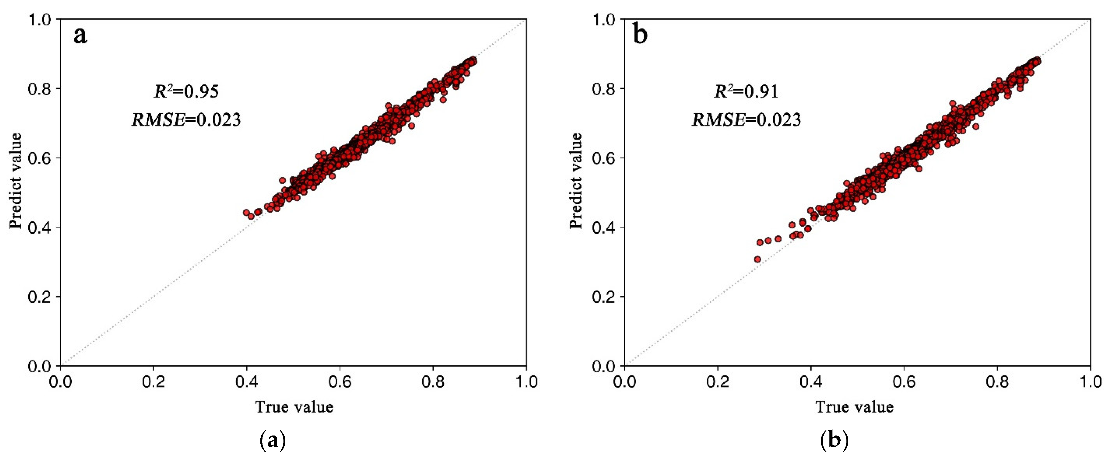
3.1. Random Forest Algorithm
3.2. Vegetation Distribution Mapping Based on GEE Platform
3.3. Thiel–Sen/Mann–Kendall Trend-Testing Approach
3.4. The Relationship between VG and Climate Factors
4. Results
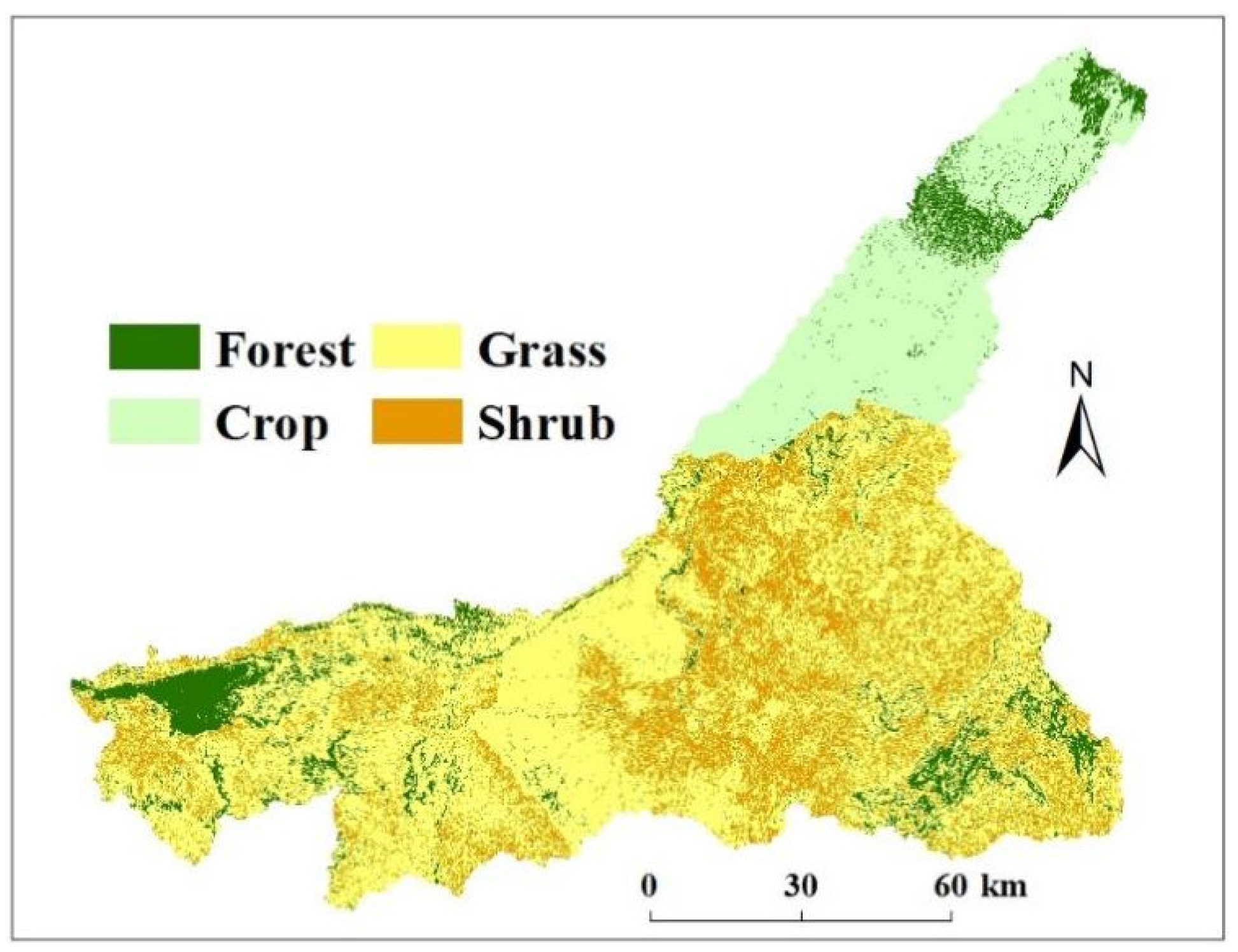
4.1. Vegetation Distribution Mapping of Mara River Basin
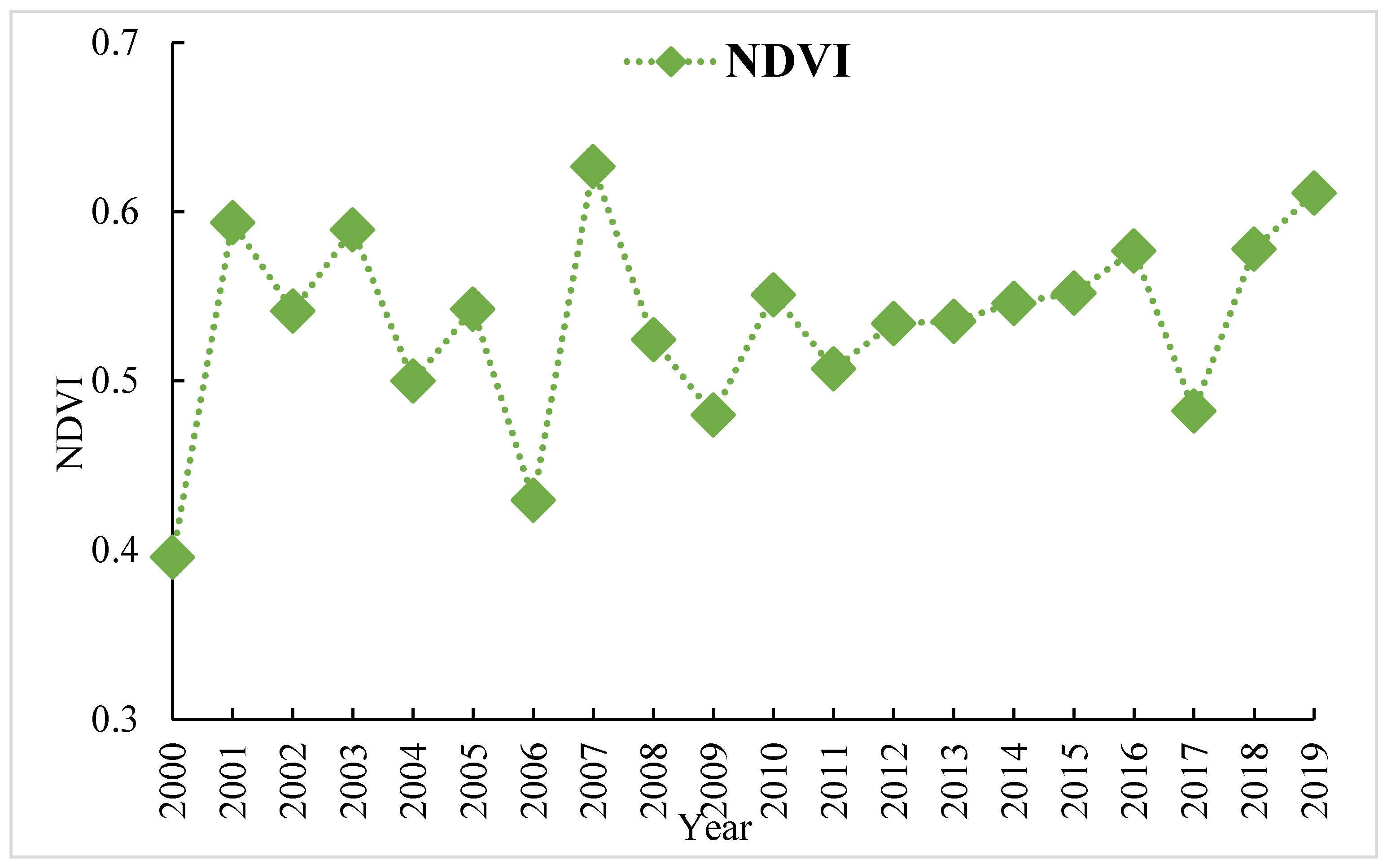
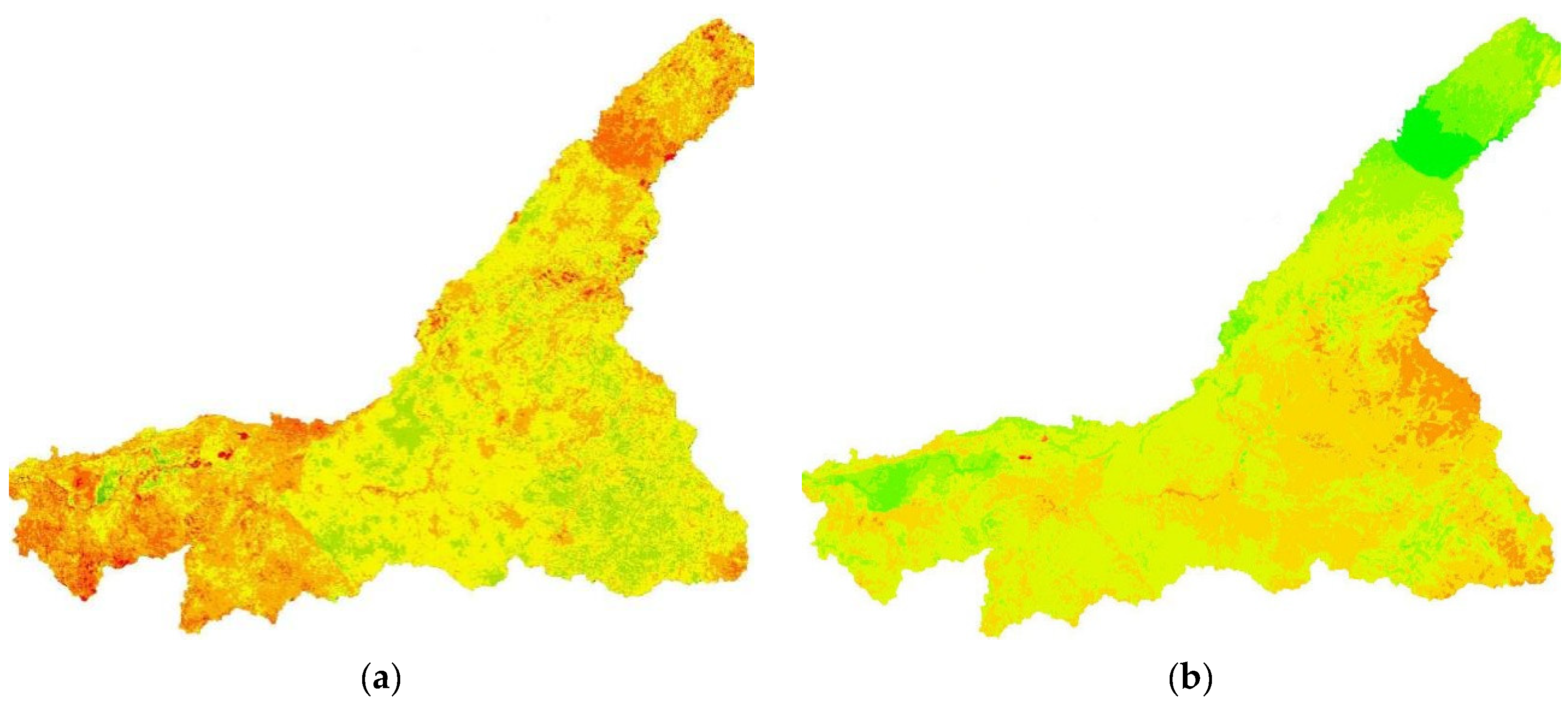
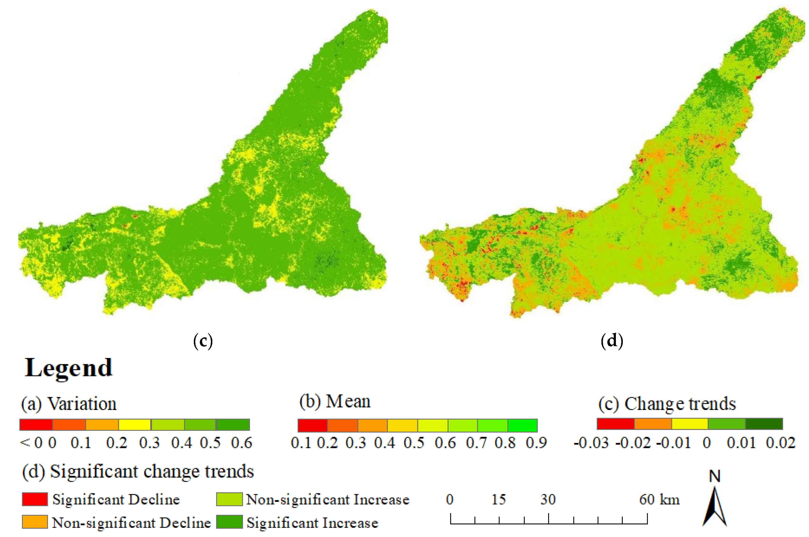
4.2. Spatiotemporal Trend of VG in Dry Seasons
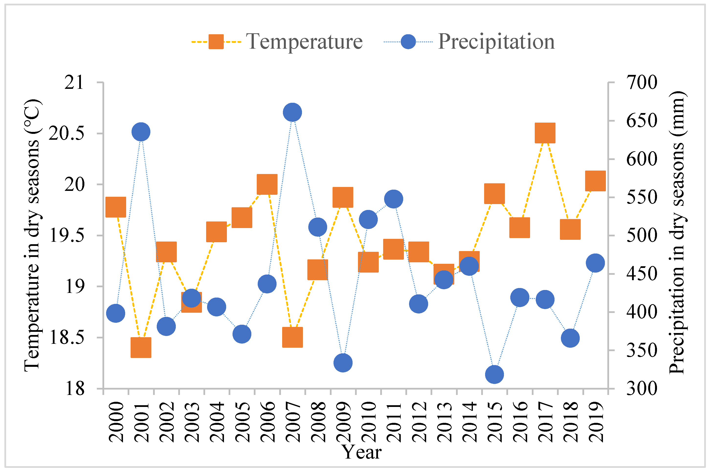
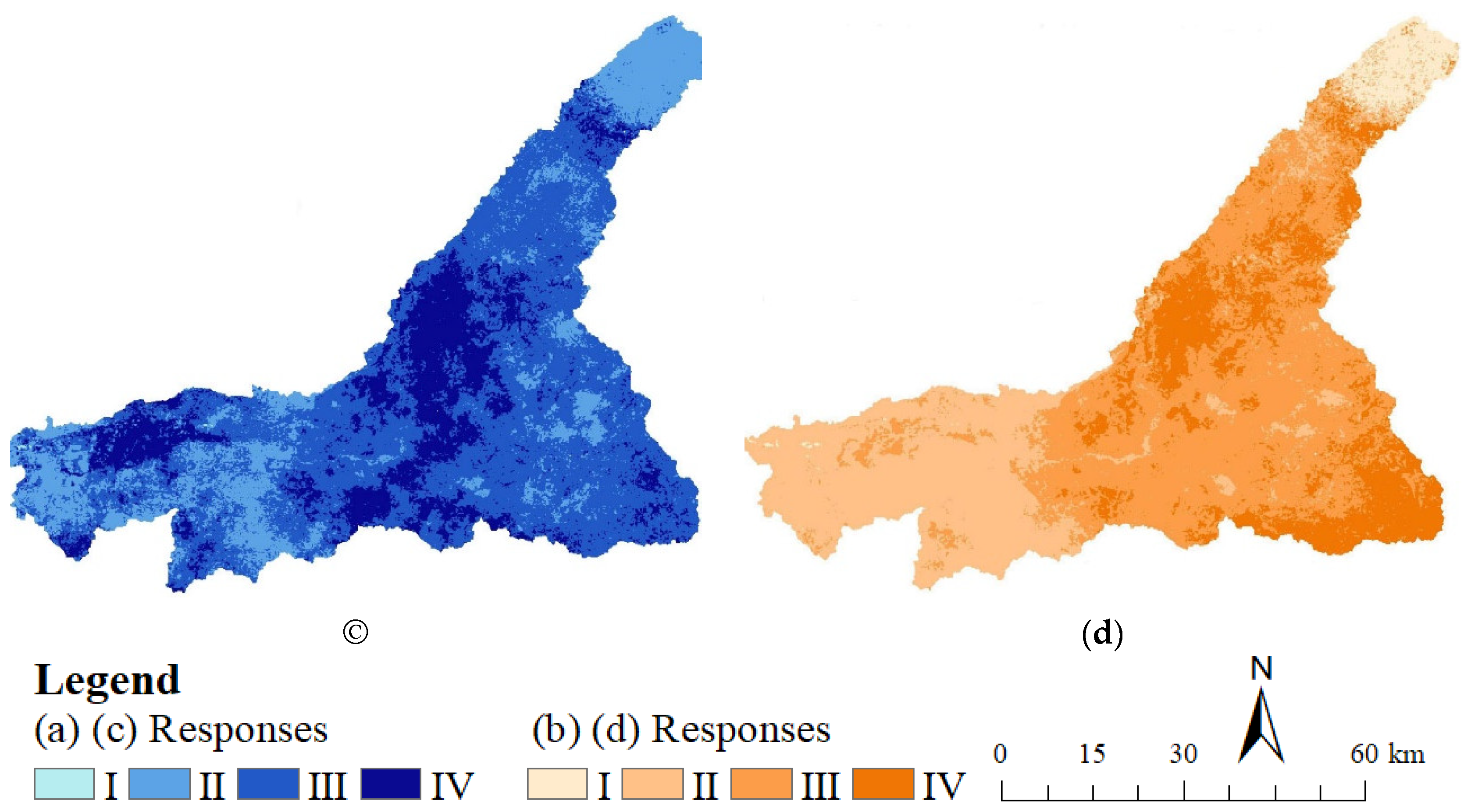
4.3. Responses of VG and VGT to Climate Change in Dry Seasons
5. Discussion
6. Conclusions
Author Contributions
Funding
Institutional Review Board Statement
Informed Consent Statement
Data Availability Statement
Acknowledgments
Conflicts of Interest
References
- Lamchin, M.; Wang, S.W.; Lim, C.H.; Ochir, A.; Pavel, U.; Gebru, B.M.; Choi, Y.; Jeon, S.W.; Lee, W.K. Understanding global spatio-temporal trends and the relationship between vegetation greenness and climate factors by land cover during 1982–2014. Glob. Ecol. Conserv. 2020, 24, e01299. [Google Scholar] [CrossRef]
- Nicholson, S.E.; Davenport, M.L.; Malo, A.R. A comparison of the vegetation response to rainfall in the Sahel and East Africa, using normalized difference vegetation index from NOAA AVHRR. Clim. Chang. 1990, 17, 209–241. [Google Scholar] [CrossRef]
- Li, W.; Buitenwerf, R.; Munk, M.; Amoke, I.; Bøcher, P.K.; Svenning, J.C. Accelerating savanna degradation threatens the Maasai Mara socio-ecological system. Glob. Environ. Chang. 2020, 60, 102030. [Google Scholar] [CrossRef]
- Sankaran, M.; Hanan, N.P.; Scholes, R.J.; Ratnam, J.; Augustine, D.J.; Cade, B.S.; Gignoux, J.; Higgins, S.I.; Le Roux, X.; Ludwig, F.; et al. Determinants of woody cover in African savannas. Nature 2005, 438, 846–849. [Google Scholar] [CrossRef] [PubMed]
- Ghebrezgabher, M.G.; Yang, T.; Yang, X.; Eyassu Sereke, T. Assessment of NDVI variations in responses to climate change in the Horn of Africa. Egypt. J. Remote Sens. Space Sci. 2020, 23, 249–261. [Google Scholar] [CrossRef]
- Musau, J.; Patil, S.; Sheffield, J.; Marshall, M. Spatio-temporal vegetation dynamics and relationship with climate over East Africa. Hydrol. Earth Syst. Sci. Discuss. 2016, 502, 1–30. [Google Scholar]
- Barbosa, H.A.; Lakshmi Kumar, T.V.; Silva, L.R.M. Recent trends in vegetation dynamics in the South America and their relationship to rainfall. Nat. Hazards 2015, 77, 883–899. [Google Scholar] [CrossRef]
- Dhillon, M.S.; Dahms, T.; Kübert-Flock, C.; Steffan-Dewenter, I.; Zhang, J.; Ullmann, T. Spatiotemporal Fusion Modelling Using STARFM: Examples of Landsat 8 and Sentinel-2 NDVI in Bavaria. Remote Sens. 2022, 14, 677. [Google Scholar] [CrossRef]
- Chakhar, A.; Hernández-López, D.; Ballesteros, R.; Moreno, M.A. Improving the accuracy of multiple algorithms for crop classification by integrating sentinel-1 observations with sentinel-2 data. Remote Sens. 2021, 13, 243. [Google Scholar] [CrossRef]
- Khoirunnisa, F.; Wibowo, A. Using NDVI algorithm in Sentinel-2A imagery for rice productivity estimation (Case study: Compreng sub-district, Subang Regency, West Java). IOP Conf. Ser. Earth Environ. Sci. 2020, 481, 012064. [Google Scholar] [CrossRef]
- Ma, C.; Johansen, K.; McCabe, M.F. Monitoring Irrigation Events and Crop Dynamics Using Sentinel-1 and Sentinel-2 Time Series. Remote Sens. 2022, 14, 1205. [Google Scholar] [CrossRef]
- Mao, D.; Wang, Z.; Luo, L.; Ren, C. Integrating AVHRR and MODIS data to monitor NDVI changes and their: Relationships with climatic parameters in Northeast China. Int. J. Appl. Earth Obs. Geoinf. 2012, 18, 528–536. [Google Scholar] [CrossRef]
- Kawamura, K.; Akiyama, T.; Yokota, H.; Tsutsumi, M.; Yasuda, T.; Watanabe, O.; Wang, G.; Wang, S. Monitoring of forage conditions with MODIS imagery in the Xilingol steppe, Inner Mongolia. Int. J. Remote Sens. 2005, 26, 1423–1436. [Google Scholar] [CrossRef]
- Petus, C.; Lewis, M.; White, D. Monitoring temporal dynamics of Great Artesian Basin wetland vegetation, Australia, using MODIS NDVI. Ecol. Indic. 2013, 34, 41–52. [Google Scholar] [CrossRef]
- Walker, D.A.; Epstein, H.E.; Raynolds, M.K.; Kuss, P.; Kopecky, M.A.; Frost, G.V.; Danils, F.J.A.; Leibman, M.O.; Moskalenko, N.G.; Matyshak, G.V.; et al. Environment, vegetation and greenness (NDVI) along the North America and Eurasia Arctic transects. Environ. Res. Lett. 2012, 7, 015504. [Google Scholar] [CrossRef] [Green Version]
- Ju, J.; Masek, J.G. The vegetation greenness trend in Canada and US Alaska from 1984–2012 Landsat data. Remote Sens. Environ. 2016, 176, 1–16. [Google Scholar] [CrossRef]
- Hmimina, G.; Dufrêne, E.; Pontailler, J.Y.; Delpierre, N.; Aubinet, M.; Caquet, B.; de Grandcourt, A.; Burban, B.; Flechard, C.; Granier, A.; et al. Evaluation of the potential of MODIS satellite data to predict vegetation phenology in different biomes: An investigation using ground-based NDVI measurements. Remote Sens. Environ. 2013, 132, 145–158. [Google Scholar] [CrossRef]
- Potter, C. Recovery rates of Wetland Vegetation Greenness in severely burned ecosystems of Alaska derived from satellite image analysis. Remote Sens. 2018, 10, 1456. [Google Scholar] [CrossRef] [Green Version]
- Fang, X.; Zhu, Q.; Ren, L.; Chen, H.; Wang, K.; Peng, C. Large-scale detection of vegetation dynamics and their potential drivers using MODIS images and BFAST: A case study in Quebec, Canada. Remote Sens. Environ. 2018, 206, 391–402. [Google Scholar] [CrossRef]
- Wang, Z.; Liu, X.; Wang, H.; Zheng, K.; Li, H.; Wang, G.; An, Z. Monitoring vegetation greenness in response to climate variation along the elevation gradient in the three-river source region of China. ISPRS Int. J. Geo-Inf. 2021, 10, 193. [Google Scholar] [CrossRef]
- Gillespie, T.W.; Ostermann-Kelm, S.; Dong, C.; Willis, K.S.; Okin, G.S.; MacDonald, G.M. Monitoring changes of NDVI in protected areas of southern California. Ecol. Indic. 2018, 88, 485–494. [Google Scholar] [CrossRef]
- Touhami, I.; Moutahir, H.; Assoul, D.; Bergaoui, K.; Aouinti, H.; Bellot, J.; Andreu, J.M. Multi-year monitoring land surface phenology in relation to climatic variables using MODIS-NDVI time-series in Mediterranean forest, Northeast Tunisia. Acta Oecologica 2022, 114, 103804. [Google Scholar] [CrossRef]
- Couteron, P.; Kokou, K. Woody vegetation spatial patterns in a semi-arid savanna of Burkina Faso, West Africa. Plant Ecol. 1997, 132, 211–227. [Google Scholar] [CrossRef]
- Mutiti, C.M.; Medley, K.E.; Mutiti, S. Using GIS and remote sensing to explore the influence of physical environmental factors and historical land use on bushland structure. Afr. J. Ecol. 2017, 55, 477–486. [Google Scholar] [CrossRef]
- Ogutu, J.O.; Piepho, H.P.; Dublin, H.T.; Bhola, N.; Reid, R.S. El Niño-Southern Oscillation, rainfall, temperature and Normalized Difference Vegetation Index fluctuations in the Mara-Serengeti ecosystem. Afr. J. Ecol. 2008, 46, 132–143. [Google Scholar] [CrossRef]
- Li, W.; Buitenwerf, R.; Munk, M.; Bøcher, P.K.; Svenning, J.C. Deep-learning based high-resolution mapping shows woody vegetation densification in greater Maasai Mara ecosystem. Remote Sens. Environ. 2020, 247, 111953. [Google Scholar] [CrossRef]
- Ogutu, J.O.; Owen-Smith, N. ENSO, rainfall and temperature influences on extreme population declines among African savanna ungulates. Ecol. Lett. 2003, 6, 412–419. [Google Scholar] [CrossRef]
- McClain, M.E.; Subalusky, A.L.; Anderson, E.P.; Dessu, S.B.; Melesse, A.M.; Ndomba, P.M.; Mtamba, J.O.D.; Tamatamah, R.A.; Mligo, C. Comparaison du régime d’écoulement, de l’hydraulique en rivière et des communautés biologiques en vue de déduire les relations débit-écologie de la rivière Mara au Kenya et en Tanzanie. Hydrol. Sci. J. 2014, 59, 801–819. [Google Scholar] [CrossRef]
- George Marcellus Metobwa, O. Water Demand Simulation Using WEAP 21: A Case Study of the Mara River Basin, Kenya. Int. J. Nat. Resour. Ecol. Manag. 2018, 3, 9. [Google Scholar] [CrossRef]
- WREM International Inc. Mara River Basin Monograph: Final Report; WREM International Inc.: Atlanta, GA, USA, 2008; p. 446. [Google Scholar]
- Mnaya, B.; Mtahiko, M.G.G.; Wolanski, E. The Serengeti will die if Kenya dams the Mara River. Oryx 2017, 51, 581–583. [Google Scholar] [CrossRef] [Green Version]
- Dessu, S.B.; Melesse, A.M.; Bhat, M.G.; McClain, M.E. Assessment of water resources availability and demand in the Mara River Basin. Catena 2014, 115, 104–114. [Google Scholar] [CrossRef]
- Mango, L.M.; Melesse, A.M.; McClain, M.E.; Gann, D.; Setegn, S.G. Land use and climate change impacts on the hydrology of the upper Mara River Basin, Kenya: Results of a modeling study to support better resource management. Hydrol. Earth Syst. Sci. 2011, 15, 2245–2258. [Google Scholar] [CrossRef] [Green Version]
- Zermoglio, F.; Scott, O.; Said, M.; Incs, I.C. Vulnerability and Adaptation Assessment in the Mara river basin. Who 2019, 100, 102–105. [Google Scholar]
- Breiman, L. Random forests. Mach. Learn. 2001, 45, 5–32. [Google Scholar] [CrossRef] [Green Version]
- Ho, T.K. The random subspace method for constructing decision forests. IEEE Trans. Pattern Anal. Mach. Intell. 1998, 20, 832–844. [Google Scholar] [CrossRef] [Green Version]
- Eisavi, V.; Homayouni, S.; Yazdi, A.M.; Alimohammadi, A. Land cover mapping based on random forest classification of multitemporal spectral and thermal images. Environ. Monit. Assess. 2015, 187, 291. [Google Scholar] [CrossRef] [PubMed]
- Jhonnerie, R.; Siregar, V.P.; Nababan, B.; Prasetyo, L.B.; Wouthuyzen, S. Random Forest Classification for Mangrove Land Cover Mapping Using Landsat 5 TM and Alos Palsar Imageries. Procedia Environ. Sci. 2015, 24, 215–221. [Google Scholar] [CrossRef] [Green Version]
- Davies, A.B.; Asner, G.P. Elephants limit aboveground carbon gains in African savannas. Glob. Chang. Biol. 2019, 25, 14585. [Google Scholar] [CrossRef]
- Chen, J.; Jönsson, P.; Tamura, M.; Gu, Z.; Matsushita, B.; Eklundh, L. A simple method for reconstructing a high-quality NDVI time-series data set based on the Savitzky-Golay filter. Remote Sens. Environ. 2004, 91, 332–344. [Google Scholar] [CrossRef]
- Verhoef, W. Application of harmonic analysis of NDVI time series (HANTS). Fourier Anal. Temporal NDVI S. Afr. Am. Continents. 1996, 108, 19–24. [Google Scholar]
- Hao, P.; Zhan, Y.; Wang, L.; Niu, Z.; Shakir, M. Feature selection of time series MODIS data for early crop classification using random forest: A case study in Kansas, USA. Remote Sens. 2015, 7, 5347–5369. [Google Scholar] [CrossRef] [Green Version]
- Mann, H.B. Nonparametric Tests Against Trend. Econometrica 1945, 13, 245. [Google Scholar] [CrossRef]
- Ogutu, J.O.; Owen-Smith, N.; Piepho, H.P.; Said, M.Y.; Kifugo, S.C.; Reid, R.S.; Gichohi, H.; Kahumbu, P.; Andanje, S. Changing wildlife populations in nairobi national park and adjoining athi-kaputiei plains: Collapse of the migratory wildebeest. Open Conserv. Biol. J. 2013, 7, 11–26. [Google Scholar] [CrossRef] [Green Version]
- Das, P.; Zhang, Z.; Ren, H. Evaluation of four bias correction methods and random forest model for climate change projection in the Mara River Basin, East Africa. J. Water Clim. Chang. 2022, 13, 1900–1919. [Google Scholar] [CrossRef]
- Reed, D.N.; Anderson, T.M.; Dempewolf, J.; Metzger, K.; Serneels, S. The spatial distribution of vegetation types in the Serengeti ecosystem: The influence of rainfall and topographic relief on vegetation patch characteristics. J. Biogeogr. 2009, 36, 770–782. [Google Scholar] [CrossRef]
- Dutton, C.L.; Subalusky, A.L.; Anisfeld, S.C.; Njoroge, L.; Rosi, E.J.; Post, D.M. The influence of a semi-Arid sub-catchment on suspended sediments in the Mara River, Kenya. PLoS ONE 2018, 13, e0192828. [Google Scholar] [CrossRef] [Green Version]
- Bregoli, F.; Crosato, A.; Paron, P.; McClain, M.E. Humans reshape wetlands: Unveiling the last 100 years of morphological changes of the Mara Wetland, Tanzania. Sci. Total Environ. 2019, 691, 896–907. [Google Scholar] [CrossRef]
- Mwemezi, B.R.; Luvara, V.G.M. Reliability of the Environmental Feasibility Studies to the Mining and Construction Projects: A Case of Mara River Basin in Tanzania. Am. J. Environ. Eng. 2017, 7, 65–72. [Google Scholar] [CrossRef]
- Pruijssen, M.J. FLEX-Topo Modelling of Water Use and Demand in the Mara River Basin, Kenya; Delft University of Technology: Delft, The Netherlands, 2015. [Google Scholar]
- Bartzke, G.S.; Ogutu, J.O.; Mukhopadhyay, S.; Mtui, D.; Dublin, H.T.; Piepho, H.P. Rainfall trends and variation in the Maasai Mara ecosystem and their implications for animal population and biodiversity dynamics. PLoS ONE 2018, 13, e0202814. [Google Scholar] [CrossRef]
- Wainwright, C.M.; Black, E.; Allan, R.P. Future Changes in Wet and Dry Season Characteristics in CMIP5 and CMIP6 simulations. J. Hydrometeorol. 2021, 9, 2339–2356. [Google Scholar] [CrossRef]
- Ogutu, J.O.; Owen-Smith, N. Oscillations in large mammal populations: Are they related to predation or rainfall? Proc. Afr. J. Ecol. 2005, 43, 332–339. [Google Scholar] [CrossRef]
- Sintayehu, D.W. Impact of climate change on biodiversity and associated key ecosystem services in Africa: A systematic review. Ecosyst. Health Sustain. 2018, 4, 225–239. [Google Scholar] [CrossRef] [Green Version]
- Brown, J.D. Biogeography, Sinauer Associates; TTESOL International Association: Alexandria, VA, USA, 2013; Volume 17, pp. 44–50. [Google Scholar]
- Thuiller, W.; Broennimann, O.; Hughes, G.; Alkemade, J.R.M.; Midgley, G.F.; Corsi, F. Vulnerability of African mammals to anthropogenic climate change under conservative land transformation assumptions. Glob. Chang. Biol. 2006, 12, 424–440. [Google Scholar] [CrossRef]
- Barros, V.R.; Field, C.B.; Dokken, D.J.; Mastrandrea, M.D.; Mach, K.J.; Bilir, T.E.; Chatterjee, M.; Ebi, K.L.; Estrada, Y.O.; Genova, R.C.; et al. Climate Change 2014 Impacts, Adaptation, And Vulnerability Part B: Regional Aspects: Working Group II Contribution to The Fifth Assessment Report of The Intergovernmental Panel On Climate Change; Cambridge University Press: Cambridge, UK, 2014; ISBN 9781107415386. [Google Scholar]
- Walther, G.R.; Post, E.; Convey, P.; Menzel, A.; Parmesan, C.; Beebee, T.J.C.; Fromentin, J.M.; Hoegh-Guldberg, O.; Bairlein, F. Ecological responses to recent climate change. Nature 2002, 416, 389–395. [Google Scholar] [CrossRef] [PubMed]
- Root, T.L.; Price, J.T.; Hall, K.R.; Schneider, S.H.; Rosenzweig, C.; Pounds, J.A. Fingerprints of global warming on wild animals and plants. Nature 2003, 421, 57–60. [Google Scholar] [CrossRef] [PubMed]


| Change Trend | Forest | Crop | Grass | Shrub | Total Area (km2) |
|---|---|---|---|---|---|
| Significant Decline | 2.02 | 1.20 | 2.62 | 2.47 | 312.10 |
| Non-significant Decline | 6.58 | 7.72 | 16.12 | 19.73 | 1950.59 |
| Non-significant Increase | 37.54 | 46.34 | 68.62 | 74.44 | 8547.90 |
| Significant Increase | 53.87 | 44.74 | 12.64 | 3.36 | 2939.57 |
| Total Area (km2) | 1541.68 | 2488.49 | 7214.55 | 2505.44 | 13,750.16 |
| Vegetation | r | Temperature | Precipitation |
|---|---|---|---|
| Forest | 0.42 | 25.68(−) | 35.36(+) |
| Crop | 0.28 | 30.65(−) | 70.23(+) |
| Grass | 0.62 | 18.78(+) | 60.04(+) |
| Shrub | 0.45 | 22.43(+) | 47.55(+) |
| Vegetation | r | Temperature | Precipitation |
|---|---|---|---|
| Forest | 0.36 | 40.10(−) | 27.46(−) |
| Crop | 0.42 | 26.64(−) | 70.23(+) |
| Grass | 0.57 | 44.81(−) | 34.64(+) |
| Shrub | 0.48 | 42.27(−) | 50.48(n) |
Publisher’s Note: MDPI stays neutral with regard to jurisdictional claims in published maps and institutional affiliations. |
© 2022 by the authors. Licensee MDPI, Basel, Switzerland. This article is an open access article distributed under the terms and conditions of the Creative Commons Attribution (CC BY) license (https://creativecommons.org/licenses/by/4.0/).
Share and Cite
Zhu, W.; Zhang, Z.; Zhao, S.; Guo, X.; Das, P.; Feng, S.; Liu, B. Vegetation Greenness Trend in Dry Seasons and Its Responses to Temperature and Precipitation in Mara River Basin, Africa. ISPRS Int. J. Geo-Inf. 2022, 11, 426. https://doi.org/10.3390/ijgi11080426
Zhu W, Zhang Z, Zhao S, Guo X, Das P, Feng S, Liu B. Vegetation Greenness Trend in Dry Seasons and Its Responses to Temperature and Precipitation in Mara River Basin, Africa. ISPRS International Journal of Geo-Information. 2022; 11(8):426. https://doi.org/10.3390/ijgi11080426
Chicago/Turabian StyleZhu, Wanyi, Zhenke Zhang, Shuhe Zhao, Xinya Guo, Priyanko Das, Shouming Feng, and Binglin Liu. 2022. "Vegetation Greenness Trend in Dry Seasons and Its Responses to Temperature and Precipitation in Mara River Basin, Africa" ISPRS International Journal of Geo-Information 11, no. 8: 426. https://doi.org/10.3390/ijgi11080426
APA StyleZhu, W., Zhang, Z., Zhao, S., Guo, X., Das, P., Feng, S., & Liu, B. (2022). Vegetation Greenness Trend in Dry Seasons and Its Responses to Temperature and Precipitation in Mara River Basin, Africa. ISPRS International Journal of Geo-Information, 11(8), 426. https://doi.org/10.3390/ijgi11080426