Article

Multi-Criterion Spatial Optimization of Future Police Stations Based on Urban Expansion and Criminal Behavior Characteristics

School of Environment Science and Spatial Informatics, China University of Mining and Technology, Xuzhou 221116, China
*
Author to whom correspondence should be addressed.
ISPRS Int. J. Geo-Inf. 2022, 11(7), 384; https://doi.org/10.3390/ijgi11070384
Submission received: 1 May 2022 / Revised: 26 June 2022 / Accepted: 4 July 2022 / Published: 11 July 2022

Abstract

:
Lanzhou’s rapid development has raised new security challenges, and improving public safety in areas under the jurisdiction of police stations is an effective way to address the problem of public security in urban areas. Unfortunately, the existing studies do not consider how factors such as future land changes, building functions, and characteristics of criminal behavior influence the choice of areas for police stations and the optimization of police stations with respect to traffic congestion. To solve these problems, we apply multiple methods and multi-source geospatial data to optimize police station locations. The proposed method incorporates a big data perspective, which provides new ideas and technical approaches to site selection models. First, we use the central city of Lanzhou as the study area and erase the exclusion areas from the initial layer to identify the undeveloped areas. Second, historical crime data, point of interest, and other data are combined to assess the potential crime risk. We then use the analytic hierarchy process to comprehensively assess undeveloped areas based on potential crime hotspots and on socioeconomic drivers and orography. In addition, according to China’s Road Traffic Safety Law and the current traffic congestion in the city, a minimum speed is determined, so that the target area can be reached in time even in congested traffic. Finally, we draw the spatial coverage map of police stations based on the location-allocation model and network analysis and optimize the map by considering the coverage rate of high-risk areas and building construction, in addition to maintenance and other objectives. The result shows that crime concentrates mainly in densely populated areas, indicating that people and wealth are the main drivers of crime. The differences in the spatial distribution of crime hotspots and residential areas at different spatial scales mean that the ratio of public security police force to household police force allocated to different police stations is spatially nonuniform. The method proposed herein reduces the overlap of police station service areas by 22.8% and increases the area coverage (12.01%) and demand point coverage (7.25%). The area coverage means an area potentially accessible within five minutes, and point coverage implies an effective drive. Within reasonable optimization, this allows us to eventually remove 13 existing police stations and add 24 candidate police stations.

1. Introduction

In China, the demand for public services in cities is increasing [1] in this era of rapid economic development in China, along with the concomitant increase in uncertain factors, such as city expansion and compactness. Fortunately, urban development has slowed in recent years, and urban resources are largely being used to improve the quality of urban public services [2]. Public security is one of the critical services provided by metropolitan areas and is one of the essential considerations for the high-quality development of urban areas. The police station is the basis of China’s public security system. Its primary responsibility is to prevent and control the occurrence and expansion of public security accidents and maintain social stability. At the same time, police stations have basic responsibilities, and multiple tasks are performed by the police officers involved, so police stations should be adequately distributed spatially. Inadequate public security seriously affects the personal and property safety of residents. From 2001 to 2021, the cumulative number of criminal offenses exceeded 10 million, as shown in Figure 1. Note that these data only cover mainland China and do not include Hong Kong, Macao, or Taiwan. In 2021, the procuratorate prosecuted over 1.74 million people for criminal offenses. Of these, 350,000 were charged with dangerous driving, 200,000 were charged with theft, and 110,000 were charged with fraud. In 1995, Wang stressed the necessity of optimizing the layout of urban police stations, pointing out that, due to historical reasons, the layout of police stations in China is arbitrary [3]. Some police districts overlap with others, which wastes a lot of police and financial resources. To reduce criminal incidents, a better understanding of the spatial optimization of police stations is essential. The potential risks in urban areas are increasingly complex and challenging to assess and counter because of rapid urban expansion and frequent changes in land use and roads. In addition, the traffic situation is increasingly complex due to the increase in city scale and in the density of vehicles, and traffic congestion significantly affects the accessibility of police stations. Therefore, cities urgently need a scientific and rational approach to police station site selection.
Facility location-allocation (L-A) research has a long history. The model helps determine the optimal location for one or more facilities, so that the stakeholder can use the services or goods provided by the facility in the most efficient situation [1]. Since Hakimi proposed the L-A model in 1964, it has been widely used to allocate facility locations, and scholars have contributed to improving the algorithm [4]. In 1990, Church improved the P-Median algorithm and introduced regional restriction into the model [5]. In 1997, Murrary and Gottsegen integrated the Lagrangian relaxation technique into the L-A model, considering the facility capacity constraints and the location requirements of the area restrictions [6]. In 1997, Gong et al. combined the traditional L-A technology with a genetic algorithm and evolutionary strategy to solve the problem of limited capacity of location facilities [7]. In 2001, Marianov and Serra proposed a hierarchical location model. The lower-level facilities prioritize the customers and then refer them to higher-level service facilities to address questions about sitting in crowded systems [8]. In 1998, Lozano et al. applied self-organizing feature maps to alternating L-A to obtain local optimal solutions under continuous demand [9]. In 2003, Salhi and Gamal proposed a L-A model based on a genetic algorithm to solve the constant L-A problem [10]. In 2004, Hsieh and Tien proposed the straight-line distance of self-organizing feature maps based on Kohonen to solve the L-A problem without capacity constraints [11]. In the same year, Xia and Jiaan combined genetic algorithms and geographical information systems (GIS) to solve complex spatial optimal allocation problems, and intelligent exploration methods significantly improved the spatial search ability [12]. In 2007, Qinou applied the improved clonal selection algorithm to study the general layout problem [13]. In 2016, Zhang assessed urban fire risk and fire force (i.e., fire station personnel and equipment configuration, fire station coverage) [14]. In 2021, Wang et al. used point of interest (POI) data to investigate the actual coverage of fire stations in central Beijing under different traffic conditions [15]. In the same year, Jiang et al. considered how negative factors, such as current fire risk, land cover, the spatial distribution of fire stations, and traffic congestion, affect the choice of fire station location [1]. The locations of optimized facilities are mainly divided into the following types: commercial enterprise location [16,17], fire station location [18,19,20], medical facility location [21,22,23], school location, and school district division [24,25,26]. In addition, one must consider airport locations [27], the optimal layout of rural settlements [28,29], transport-hub locations [30], refuge location [31], logistics distribution centers, etc. [32,33].
This review of previous studies shows that siting models and multi-source data have been widely used in facility siting. It is known that the location distribution of public security police stations is essentially a problem of optimal allocation of point element space. However, existing studies still have some minor problems [15]. First, due to the lack of detailed building information, existing methods usually use parcels or blocks to simulate the risk zone without distinguishing between the buildings’ functional heterogeneity. In addition, the crime risk in cities is influenced by the urban environment. Second, detailed information about the transportation network is rarely considered in site selection. Third, existing research ignores how uncertainty and the dynamic development of cities create a complex geographic system that influences the choice of facility location. Fourth, research on the location of police stations has heretofore mainly focused on police patrolling [34], police vehicle positioning [35], and police dispatching [36], whereas almost no research exists on the spatial location and spatial allocation of the police force.
These problems often mean that the final site selection cannot meet the new demands or cannot adapt to the new environment after the facility is installed. Many cities in developing countries are currently undergoing rapid development, especially large- and medium-sized cities, so the polarization effect is more pronounced. Selecting the site of a planned or soon-to-be-built facility usually takes a long time. The whole process of the facility, from design to construction to final use, may take longer than expected, which often means that the previously selected location is no longer suitable in the new environment. Therefore, we must consider the details of the city in the location model and construct a model for siting facilities with the future city in mind.
The rapid development of the internet has produced many emerging geospatial data [37,38,39], which are provided in data such as POI data, thus providing new solutions to the above challenges. POI data are the point data of real geographic entities, including longitude and latitude, address, name, and other attributes. These data are of great value for city managers and emergency responders for urban planning and analyzing emergency rescue [40,41]. POI data have the advantages of fast updating speed, explicit content, a large amount of data, comprehensive coverage, and low acquisition cost to be used for quantitative risk analysis in different functional spaces. Therefore, this study addresses the limitations of the L-A model by merging two sets of data from geospatial datasets. We use POI data to assess urban risk intensity based on criminal behavior characteristics.
This study aims to address the limitations of the existing L-A model by combining three sets of information from emerging geospatial datasets and urban dynamics. Geospatial data includes POI, crime location, and land use data. This article is organized as follows. Section 2 describes the case study. The experimental results and analysis are presented in Section 3 and discussed in Section 4. Finally, Section 5 presents the conclusions.

2. Case Study and Methodology

2.1. Overview of Research Region

Our study area is Lanzhou, Gansu province, China, which has a total area of about 13,100 km2 and is located from 102°35′ to 104°34′ E longitude and 35°34′ to 36°59′ N latitude. According to China’s seventh population census data, as of 00:00 on 1 November 2020, the resident population of Lanzhou was about 4.36 million. Lanzhou is an industrial base in China, a large-scale comprehensive transportation city, an important node city of the Silk Road Economic Belt, and has become an important inflow city for the mobile population in northwest China. The traditional culture, living habits, religious beliefs, ethnicity, and other aspects of the public in Lanzhou are diverse. Lanzhou is a multi-ethnic provincial capital city, with 56 ethnic groups in the city. Of these, the Hui Nationality people account for more than 3%. Apart from the Hui Nationality, the population of ethnic minorities accounts for 3.6% of the total population. Lanzhou has a complex and diverse landscape, with mountains, plateaus, flat rivers, river valleys, and deserts (Gobi), all of which are staggered and distributed, and the terrain slopes from southwest to northeast.
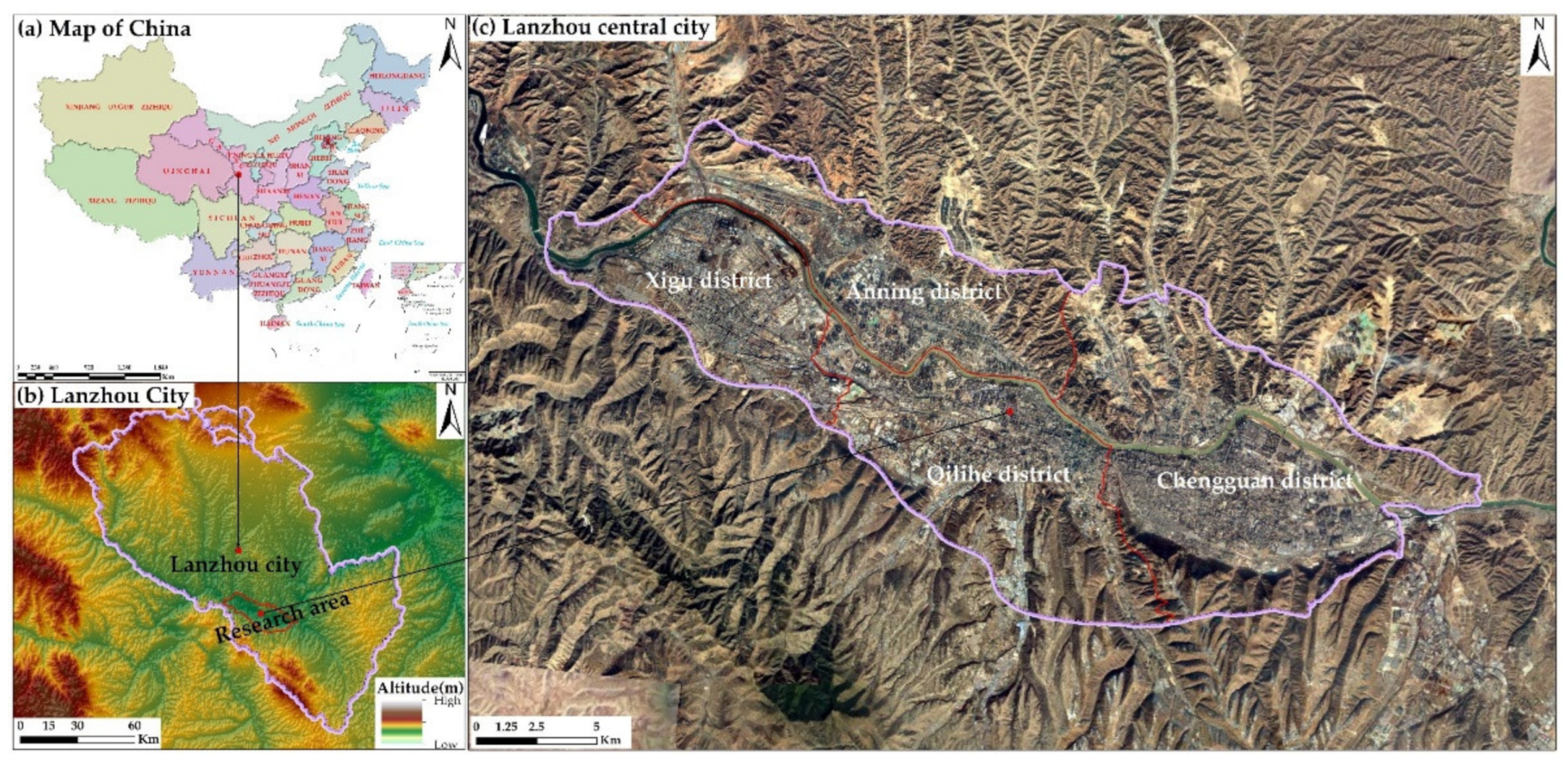
Lanzhou is also a typical river valley city. The Yellow River runs across the central urban area of Lanzhou, flowing from the southwest to the northeast, creating a landscape that divides the geographical landscape from north to south. This has implications for the extent of the city and on the potential travel times by car. The main urban area of Lanzhou consists of four districts: Chengguan District, Xigu District, Anning District, and Qilihe District. The total area of the central urban area accounts for 7.91% of the city’s total area, but 67.70% of Lanzhou’s population is concentrated in the central city area. Considering the availability of data, Lanzhou’s downtown area (Figure 2) was selected as the study area because it includes all core areas of the capital and most of the expanded urban functional areas. Lanzhou is one of the nine major logistics areas and counts 10 import logistics channels and 21 national logistics node cities. It has the densest railway network in the northwest region and is one of China’s important highway networks and railway hubs. As one of China’s comprehensive cities, Lanzhou has typical problems that most cities have, which makes it a good case study.

2.2. Methodology

This study combines tools, such as Google Earth Engine (GEE), the PLUS model, and GIS tools, used to evaluate the most suitable locations for building police stations. The proposed methodology is shown in Figure 3. First, we use historical remote-sensing images combined with potential driver data to predict future land use. Second, we use various high-resolution GIS databases to remove unsuitable layers from the initial layers. Third, we propose three evaluation criteria for the suitable areas for building police stations. Fourth, we combine hierarchical analysis and GIS to identify the most suitable areas for police stations and to create a map showing the distribution of suitable and unsuitable areas for police stations. Finally, the L-A model is used to study the spatial optimization of police stations in the study area.

2.2.1. Types of Police Station Areas

We first determine the different types of police station areas within the city. In this study, police station area types (PSATs) are classified into four categories: existing police station areas (EPSAs), existing unsuitable police station areas (EUPSAs), priority construction areas (PCAs), and not suitable for construction areas (NSCAs).
In this context, EPSA refers to the police stations that have already been built in the city. Similarly, EUPSA refers to the removal of redundant police stations within the boundaries of an existing police station. A redundant police station means that the area under the jurisdiction of that police station is already covered by a large area of its surrounding police stations, greatly reducing the economic cost and allowing the existing police station to be of maximum value. The PAC indicates areas highly suitable for building on undeveloped land, and such police stations tend to have relatively good environmental conditions. Finally, NSCA refers to existing built-up areas, such as conservation areas, residential land, and land use areas.

2.2.2. Land Expansion Strategy

The land expansion strategy (Figure 4) includes land use classification and future land use prediction. The details are given below.
(1)
Land Use Classification
Ground verification in uncertain areas was completed through Google Earth Pro and GEE, and misclassified areas were corrected by positioning and rearranging the GEE script samples. The ground truth points were used to estimate the mapping accuracy. Finally, images from Landsat-5 (TM) and Landsat-8 OLI (ETM) from 2018 to 2020 were classified into seven land use types (Table 1) by using the classification and regression tree classification algorithm, which is a popular supervised classification algorithm for spectral image remote-sensing technology [42,43,44]. Remote-sensing images were selected at Tier 1 level and processed systematically, geometrically, and topographically. Five spectral features were used to characterize typical land use categories, including normalized difference vegetation index (NDVI), normalized difference built-up index (NDBI), modified normalized difference water index (MNDWI), DEM and slope.
The producers and consumers evaluated the remote-sensing image classification, and a confusion matrix was used to calculate the kappa coefficient, classification accuracy, and total accuracy. Producer accuracy is the number of correctly identified pixels as a percentage of pixels in the classifier as the training sample of each batch. Consumers’ accuracy is the pixels that were accurately classified as a percentage of the total number of pixels identified as that class. The total accuracy is the ratio of the total number of correctly assigned pixels to the total number. The kappa coefficient is as follows.
K a p p a   C o e f f i c i e n t = N i n X i i i m ( X i + X + i ) N 2 i m ( X i X + i )
(2)
Prediction of Future Land Use
The PLUS model was developed by Xun et al. [45] and is suitable for scenario simulation research on future land use changes. The proposed model achieved a higher simulation accuracy and landscape pattern metrics [45]. In this study, the natural growth area of land types in the study area was estimated by modifying the input parameters of the PLUS model. The natural growth scenario refers to the real change of land use type without considering the actual situation or national policy for the time being.
The operation of the PLUS composite model includes the following aspects:
(a)
Input land use development potential drivers and remote-sensing classification data. The development potential drivers data include land use, socioeconomic drivers, and climatic and environmental drivers (Table 2). Managed-land-use-driven shaded raster files have a uniform resolution of 30 m due to the capabilities of the model calculator. Training using random forest classification so that quantitative information on how various drivers influence the expansion of multiple land use types is directly provided. Considering that the driving force of land use change may change with time (i.e., the change of driving factors), the transfer rules obtained in the training process are more valuable and more flexible than the allocation rules mined in the past. Because the transition rules in this study are time dependent, they can describe the nature of land use change in a specific time interval [46]. This advantage can help policymakers understand how drivers (e.g., the growth of arterial roads) affect short-term land use change. Therefore, the model produces more reliable simulation results for different scenarios in the future. Spatial layout is mainly influenced by topography, the natural environment, markets, government public facilities, water resources, cities, and other spatial factors [47,48,49,50]. So, based on previous studies and the current situation of the study area, we selected 3 evaluation criteria and 12 sub-criteria for the impact factors. Driving factors collected from different time periods are allowed [51], but we made the time periods of the driving factors as close as possible to the time periods of the land use data.
(b)
Setting of the restricted area. According to the actual situation of the study area and the ecological function of protected areas, museums, roads, and zoos are selected as restricted areas, and conversion to other types of land use is prohibited.
(c)
Calculate the future land demands. Based on the collected remote-sensing image data, this study uses the Markov model to calculate the future land use situation.
(d)
Set the transition matrix and neighborhood weights. Consider the impact of factors such as laws and policies and identify the type of land to be converted in the initial layer (refer also to the transition matrix). Neighborhood weights are assigned according to the normalized value of land expansion from the previous stage:
W i = T A i T A min T A max T A min
where W i is the domain weight of land use type i, T A i is the expansion area of land use type i, T A min is the minimum expansion area of all types of land use, and T A max is the maximum expansion area of various land use types.
By analyzing the actual geographical coverage of the study area, the following land use factors are considered desirable (Table 3): (i) Forestry. According to the definition of the “Forest Law of the People’s Republic of China,” the state implements a comprehensive protection system for natural forests. The system strictly limits the logging of natural forests, strengthens the capacity of natural forest management and protection, protects and restores natural forest resources, and gradually improves the ecological function of natural forests. Therefore, converting natural forests into other land use types is difficult. (ii) Waterbody. Water is the basis for the survival of life on earth, and water resources are the primary condition for maintaining the sustainable development of the earth’s ecological environment. China has severe water scarcity, and it is challenging to convert water bodies to other land types. (iii) Cropland. The ministry of land and resources has set a red line to protect permanent basic farmland to ensure national food security and improve the total grain production capacity. Therefore, cultivated land cannot be destroyed.

2.2.3. Global Moran’s Index

Since crime hotspots may have a continuous distribution in space, this paper uses this index [52] to test the spatial autocorrelation of crime hotspots within the study area [53,54], and the index is calculated as follows:
I = n S 0 i = 1 n j = 1 n w i j Z i Z j i = 1 n Z i 2
where Z i is the deviation of the attribute value of element i from the average value ( x i X ¯ ) ; w i , j denotes the spatial weights between elements i and j; n is the total number of elements; and
S 0 = i = 1 n j = 1 n w i , j
Global Moran’s I is tested for significance using the Z test calculation formula as
Z [ I ] = i E [ I ] V [ I ]
where Z [ I ] is the Z test value of the Global Moran’s I; E [ I ] is the mathematical expectation; V [ I ] is the variance.
Usually, I is between −1.0 and 1.0. When I [ 1 , 0 ) , there is a negative spatial correlation. The closer the value of I is to −1, the greater the difference in attribute values between spatial units. When I = 0, the spatial distribution is random. As I approaches 0, the attribute values between spatial units become increasingly uncorrelated. When I ( 0 , 1 ] , the correlation is spatially positive, and the closer it is to 1 means that the attribute values between spatial units are more correlated.

2.2.4. Analytic Hierarchy Process

Choosing the most suitable evaluation system is a complicated problem that requires selecting different evaluation indicators, scientifically analyzing their weight, and deriving the most suitable solution. To address this problem, researchers often use the MCDM method [55,56]. MCDM is a widely used technology in the research community and allows researchers to choose the best option based on numerous criteria [57].
Of the numerous MCDM methods available, the AHP, developed by Saaty in 1977 [55], is the most used method to solve complex decisions involving many different criteria and is a popular tool for multi-standard decision making [55,56]. The AHP is a mathematical and psychological research technique based on a series of pairwise comparisons to determine a standard weighting [58]. In addition, the AHP ensures consistent decision making and reduces deviations in the decision-making analyses. Therefore, the AHP method is used to determine the weight of evaluation criteria for searching for fire brigade sites. At the beginning of each AHP, goals, alternatives, and standards must be defined, following which a pairwise comparison matrix M is generated.
Assuming that there are N criteria to determine the number of comparisons, the specific steps for applying AHP technology are as follows [59].
A pairwise comparison matrix A (n × n) is established according to the expert’s judgment, where the element aij represents the intensity of importance of the standard i to standard j. Therefore, aji is the reciprocal of aij, representing the relative importance of standard j to standard i. The numerical scale 1–9 serves to measure the relative importance of pairwise comparisons, as shown in Table 4 [59], where “1” means equal importance of one standard relative to the other, and “9” means extreme importance of one standard relative to the other. Please refer to Ref. [59] for a more detailed explanation of the score.
To ensure the consistency of the calculated weights, pairwise comparisons need to be verified by the consistency ratio (CR). The formula is derived as follows:
i.
Calculate the maximum eigenvalue λ max of each comparison matrix.
ii.
Calculate the consistency index (CI) value by using
C I = ( λ max n ) / ( n 1 )
where λ max is the maximum eigenvalue of each comparison matrix, and n is the number of criteria or order matrix A.
iii.
Use Table 5 and the number n of standards used to obtain the random consistency index (RI) and then determine the CR by calculating the ratio of the CI to the RI:
C R = C I / R I
The CR reflects the correctness of the program. When CR ≤ 0.1, the level of consistency is acceptable. If CR ≥ 0.1, the AHP may provide significant results [60]. RI represents the average deviation of randomly generated matrices of different sizes. After excluding restricted areas, the selected criteria serve to calculate and classify suitable sites. The CR for all comparisons is less than 0.1, which means that the results are satisfactory.

2.2.5. Location Allocation Standard and Model

(1)
Location Allocation Standard. Before selecting a site, a preliminary analysis of the geospatial environment must be performed. The preliminary analysis is mainly divided into three parts, the details of which are shown below.
(i)
The NSCAs are selected. The impact of actual land use, such as protected areas, museums, roads, and zoos, is considered. Therefore, NSCAs are selected, and the unsuitable areas in the original layer are erased. The data for the protected area are obtained by interpreting remote-sensing images. The road network data come from OSM and, based on the monitoring data of Lanzhou’s geographical conditions, the original data are preprocessed by checking, editing, and modifying the topological relationship to obtain the final road network data. The road data contain a total of 12,818 nodes.
(ii)
The PCAs are selected. The suitability of undeveloped areas is evaluated by considering the main tasks of (a) potential crime hotspots, (b) socioeconomic drivers, and (c) orography. Finally, the PCAs are found through an analytic hierarchical process and a weighted linear combination model. The assessment criteria are as follows:
(a)
Potential crime hotspots. Potential crime hotspots reflect the level of danger of crime during a certain period. Police stations represent the deterrent forces, which can be static (police stations) and/or dynamic (police patrols). In 2019, the crime of stealing and fraud remained the top two criminal case categories. However, the fraction of stealing cases declined, and the fraction of fraud cases increased. The crime of “two robberies and one theft,” that is, the crime of robbery, the crime of stealing, and the crime of forcible seizure, is characterized by repeated occurrence and directly and seriously affects people’s lives and productivity. The report “China’s Blue Book on Criminalization” pointed out that economic and property-related cases have become problems in criminal governance. In particular, cases of property violations using various emerging technologies and technological means tend to expand their influence. The crime governance data of some provinces and cities indicate a unique phenomenon. For example, in the Guangxi Zhuang Autonomous Region, the number and proportion of crimes against the public (6050) and drug cases (4514) are relatively high. Therefore, we select the crime of stealing, drug trafficking, fraud, forcible seizure, and robbery in the central urban area of Lanzhou as the research sample. The crime data come from the 2014–2016 criminal judgments of public prosecutions published by China Judgment Documents Network and include 1887 thefts, 1405 cases of drug trafficking, 124 frauds, 24 robberies, and 99 cases of stealing. The total number of cases is 3539. Therefore, police stations should protect these priority areas by selecting the best routes for police patrols to respond to emergencies. Crime hotspots are thus vital factors for determining the location of police stations. We analyze crime agglomeration characteristics by Moran’s I Index and potential risk areas by crime occurrence locations.
(b)
Socioeconomic driver. According to previous academic studies, the socioeconomic driver mainly includes population, GDP, proximity to the existing police station, and potential risk areas. The potential risk areas are determined by the location where crime occurs. The main types of POIs (such as attribute functions and social activities) are listed in Table 6. The weights of the different POIs are calculated based on the proportion of crime sites.
(c)
Orography. Regarding the orography driver, the terrain strongly influences the time and cost of police station attendance, installation and maintenance of the security system, registration and training of police officers, and emergency response services. Therefore, the slope of the area near the police station determines the acceptability of the site. Flat land is more favorable than sloped land for police stations.
(iii)
Determine the target site. In this context, we must consider spatial optimization objectives related to standards and the relevant local laws, including site objectives, such as emergency response time, coverage of high-risk areas, coverage of POI points, coverage of the entire building, and coverage of future buildings.
The emergency response time depends on the layout of the various emergency facilities. After receiving an alarm, the emergency agency must arrive at the scene within the specified time. The “110 Work Rules for Police Reception” stipulates that the municipal public security police must arrive at the scene within five minutes after receiving the police order. The spatial optimization of the police station must be based on immediate response. Therefore, we use 5 min herein as the emergency response time.
In this process, the following two aspects need to be considered simultaneously. First, the speed limit for each road is determined according to the “Code for Design of Urban Road Engineering” combined with map data. Second, the police have priority on the road and are less affected by traffic rules, such as traffic priorities and traffic lights. Thus, the road network parameters, including travel time as a function of road impedance, must be set appropriately.
(2)
Location Allocation Model
After quantitatively analyzing the various risk areas, speed limits, and target sites for police stations, we use the L-A model to analyze the coverage of existing police stations in the city.
The L-A model is an effective method for selecting sites for public facilities [61,62,63,64] and has been successfully applied to select sites for emergency and public facilities [64], such as school sites [62], hospital sites [63], and fire brigade sites [14,65]. The scientific positioning of public service facilities can facilitate the operation of these facilities. For example, a well-positioned supermarket is more convenient for residents and more profitable for the supermarket. Appropriate sites enable service facilities, such as police stations and fire brigades, to provide better services and make schools more accessible for students.
Given these considerations, we use two algorithms in the L-A model: maximize coverage location (MCL) and minimize facilities coverage (LSC). The goal of MCL is to maximize the number of demand points within the maximum service radius of the facility under the condition of selecting the spatial distribution of a given number of facilities from all candidate facilities. The goal of the LSC is to maximize the number of facility demand points within the maximum service radius of the facility under the condition of selecting the fewest facilities among all service facilities. Table 7 gives the mathematical expressions for the two algorithms. The L-A parameters are explained in the literature [66,67,68].

2.2.6. Police Station Force Allocation Method

The spatial heterogeneity of the population, crime, etc., leads to different demands on the police force for each regional police station. Note that the number of police stations does not correlate with the number of police officers. According to the Chinese police classification standard, the police force of the police stations is composed of two main parts: the public security police force and the household registration police force. Therefore, to optimize the utility of police stations, we use criteria such as the number of crimes, the number of habitations, and the number of people, and use streets to spatially separate the fraction of different types of the police force from each police station.
(1)
Public security police force. The main responsibility of the public security police force is to maintain public order in the city and prevent and control the occurrence of criminal incidents. Therefore, the total number of crimes in each region is used to allocate the public security police force in the given region. The number of police officers in each police station is calculated from the ratio of the total number of criminal incidents in the street unit where the police station is located to the total number of criminal incidents in the study area:
M i j = N i × M N × i j
where M is the total number of security police in police stations in the entire study area, N is the total number of criminal incidents in the study area, i is the street unit identifier, j identifies the police station in a street unit (so i j is the total number of police stations in a street unit i), N i is the total number of criminal incidents in a street unit i, and M i j is the number of police forces in police station j of a street unit i.
(2)
Household registration police force. The main responsibility of the household registration police force is to manage household registration and identification cards. It is also the spatial point for implementing police services. Therefore, we use the distribution of habitations to reflect the population distribution and select each area’s total residential area index as the basis for the distribution of household registration police force in the given area. In the same way, the ratio of each street unit’s total residential area to the research area’s total residential area can be used to calculate the number of the household registration police force required in each police station:
P i j = Q i × P Q × i j
where P is the total number of police stations with household registration, Q is the total residential area of the study area; i identifies the street unit, j identifies the police station in a street unit (so i j is the total number of police stations in a street unit i), Q i is the total residential area in a street unit i, and P i j is the number of the household registration police officers in police station j of a street unit i.

3. Results

3.1. Future Changes in Land Use

3.1.1. Changes in Land Use

The land use classification obtained by applying the supervised classification method depends on the input training samples. To distinguish land use under different conditions, the sample size of the initial training dataset of the classifier must be sufficiently large, especially for complex land areas [69]. An accurate test sample set is thus vital to obtaining accurate classification [70]. Therefore, by using the Sentinel-1 and Sentinel-2 data provided by the European Space Agency WorldCover 10 m 2020 product and through visual observation of false-color (RGB) composite images, we strictly limit the invariant regions of these three periods and select a total of 1816 sample sets for the training sample set. Five spectral features are used to characterize typical land use categories, including the normalized difference vegetation index, the normalized difference built-up index, the modified normalized difference water index, the digital elevation model, and slope. The kappa coefficient is greater than 0.86 for all classified images, indicating almost perfect agreement with the actual terrain, as shown in Table 8.
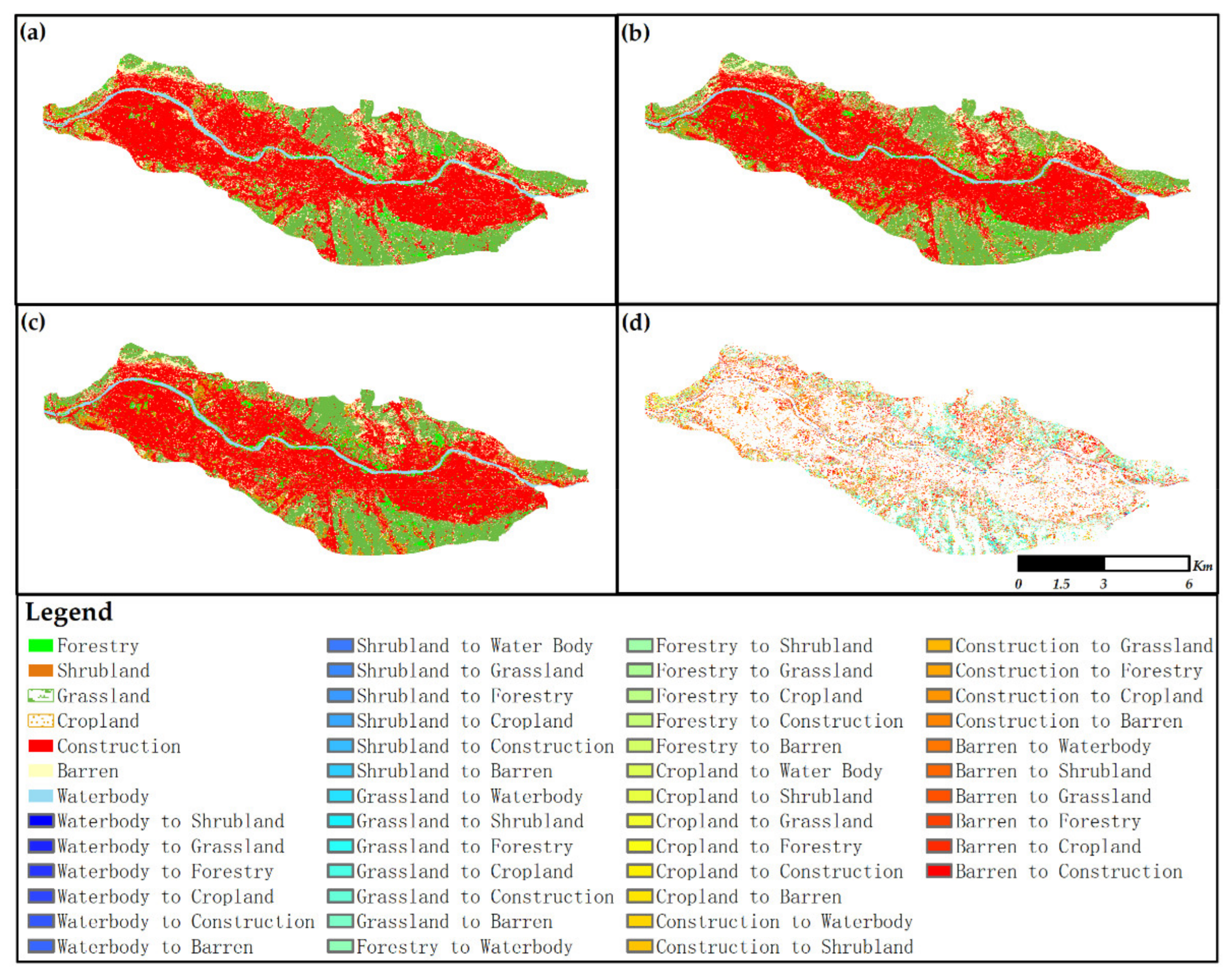
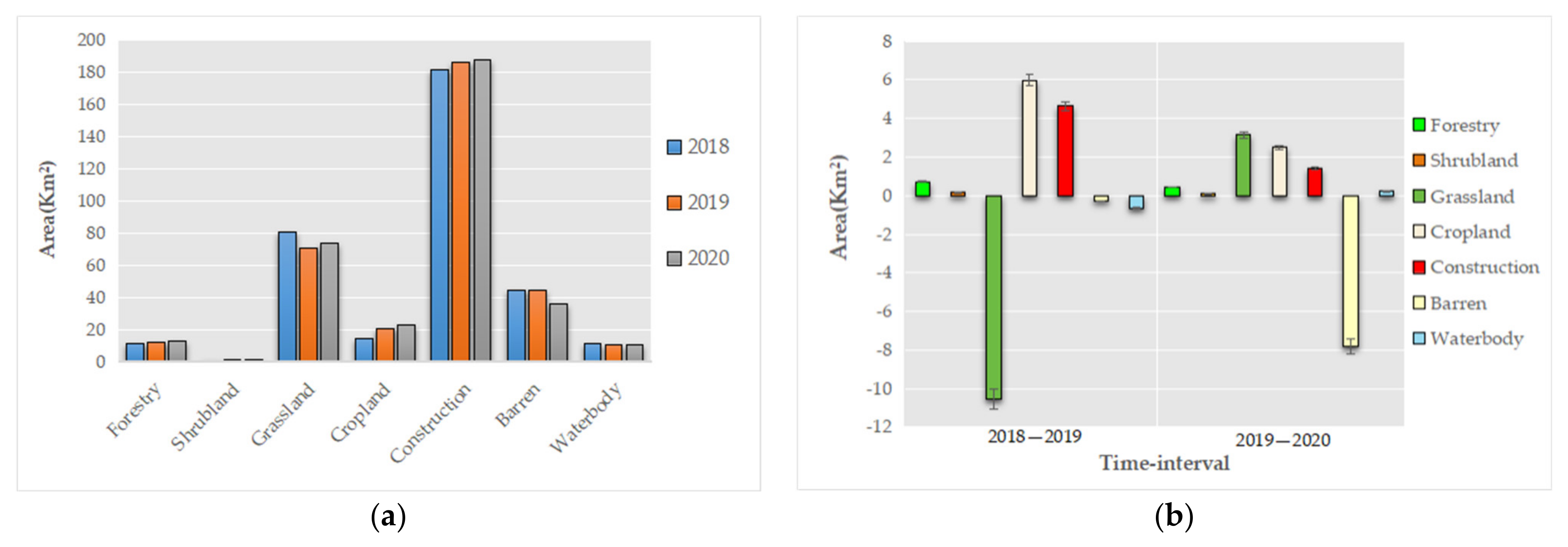
The land use classification results from Section 2.2.2 (1) are shown in Figure 5. Changes in land use are mainly concentrated in CS, CL, BA, FO, and GL. From 2018 to 2020, CS increases from 181.64 to 187.17 km2, which gives an annual change of about 2.02 km2 or 1.16% per year. This comes mainly from BA. CL increases from 14.45 to 22.92 km2, which is a net increase of 58.62%. BA decreases from 44.26 to 36.17 km2. FO increases from 11.34 to 12.5 km2, which is an increase of 10.23% and is mainly due to barren land and construction areas. From 2018 to 2020, GL decreases by 9.15%. Changes in other land use types are relatively small.
Based on the map of changes in land use (Figure 6) and the net change in all land use (Table 9), about 70% of the land use area remains unchanged from 2018 to 2020. Overall, the change in land use type in urban areas accounts for 29.82% of the area where land use changed. The area with the largest change in land use is BA (11.14%), followed by GL (5.61%). In total, 5.40% of the area in BA is converted to CL. Additionally, 1.74% of WB is converted to CL, and 1.46% of WB is converted to CS. These data show that, from 2018 to 2020, the areas of human activity rapidly replaced natural areas with semi-natural or impervious surfaces, in addition to other changes in land use. In recent years, with the support of national policies, cultivated land has received greater protection, so that the area of cultivated land grew from 2018 to 2020.

3.1.2. Simulation of Future Land Use

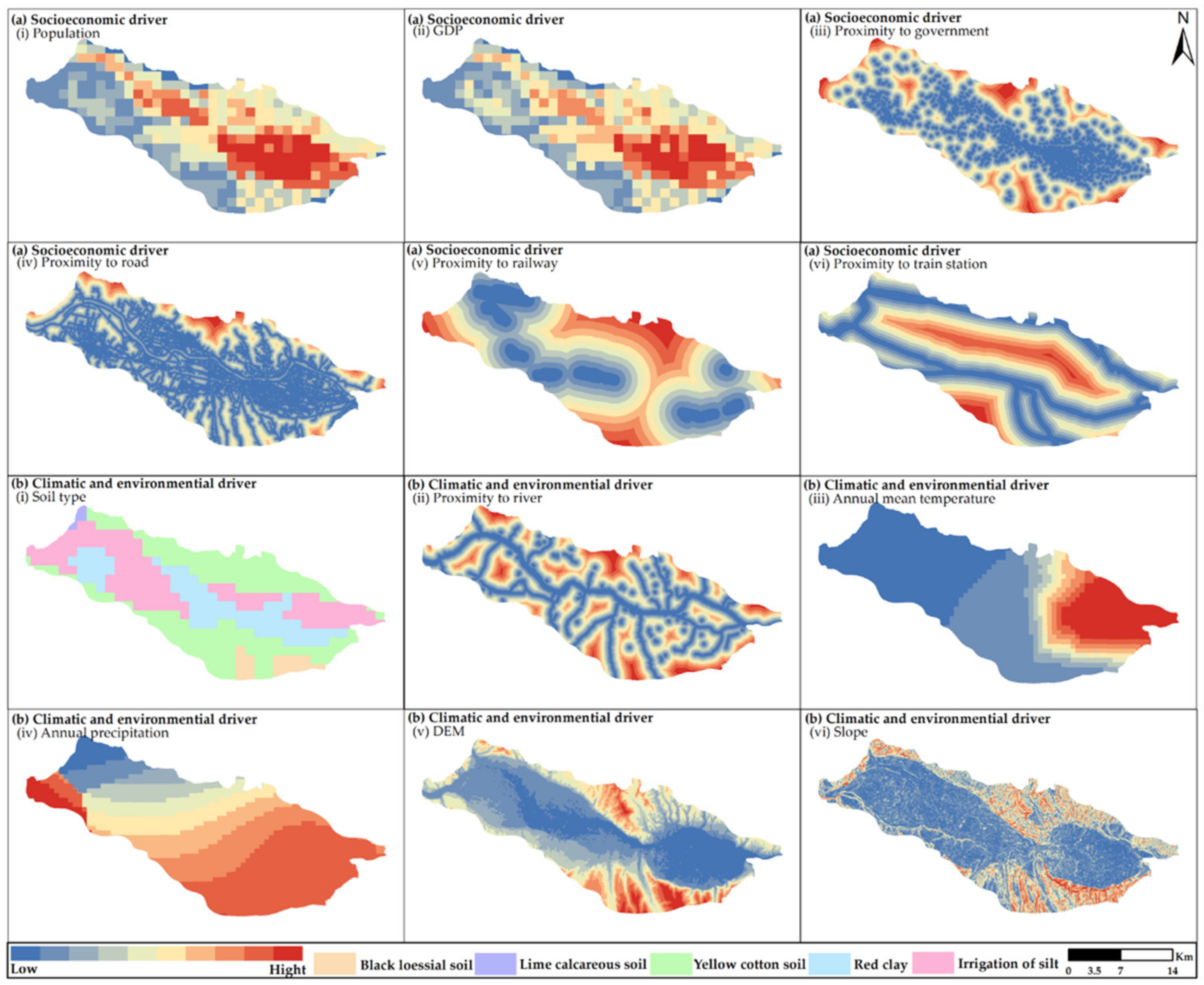
As per Section 2.2.2 (2), the evaluation criteria are divided into three criteria and twelve sub-criteria. The data processing methods used here include slope data first normalized by polarization, with all values scaled to fall within the interval [0,1]. The POI data are then spatialized by Gaussian kernel density analysis, and the road and watershed data are converted to proxy attractiveness with respect to spatial distance by using an indexed distance decay function. Figure 7 shows the spatial distribution of the various evaluation criteria. (Figure 7a(i)) The population of Lanzhou and (Figure 7a(ii)) the GDP are mainly concentrated in the Chengguan District. (Figure 7a(iii)) Government departments are evenly dispersed. (Figure 7a(iv)) Lanzhou is a central city with a dense road network. (Figure 7b(i)) The soil in Lanzhou is mainly loose and fertile loess, which is especially suitable for growing vegetables. (Figure 7b(ii)) Freshwater resources are scarce in Lanzhou, which is the only city in China through which the Yellow River passes. (Figure 7b(iii)) Lanzhou has a temperate continental climate. The average annual temperature is 10.3 °C, the annual average hours of sunshine is 2446 h, the frost-free period is 180 days, and the annual average precipitation is 327 mm, which is mainly concentrated from June to September. (Figure 7b(v)) The topography of Lanzhou is basin-like terrain, with the long, narrow city of Lanzhou sandwiched between mountains to the north and south.
As indicated in Section 2.2.2 (2), the training process of the PLUS model provides direct quantitative information on how various drivers influence the expansion of multiple land use types (Figure 8). For grassland, the results indicate that the slope has the greatest influence on grass growth, which suggests that grasses are most likely to grow in steeper areas. Forestry is more affected by proximity to water sources than grasslands. The distribution of new urban areas correlates strongly with the road pattern, which is not surprising because most urban growth depends first on the expansion of the local and the connecting road networks.
To support the Lanzhou city master plan, we use, for future simulations, the PLUS model to allocate projected land use demand at a resolution finer than the scale of local land use change. Figure 9 shows the areas of land use change from 2020 to 2030 for seven land use categories in the study area. The results of this study show that the barren area in the central city of Lanzhou has declined significantly and will continue to decline over the next 20 years, while residential areas and cropland will continue their upward trend. Thus, under the national policy, the area of cropland remains constant or continues to increase. For construction areas, more areas are added to the north.

3.2. Spatial Optimization of Police Stations

3.2.1. Exclusion Criteria

The first method to determine site selection suitability is to erase from the initial layer areas unsuitable for constructing police stations. As per Section 3.1, these exclusion criteria were determined based on insights gained from the literature, and a comprehensive list was selected for investigation. By analyzing the actual geographical coverage of the study area, the following exclusion criteria are considered desirable: land cover (EC1), transportation infrastructure (EC2), and orography (EC3). Figure 10 shows a map of the area which the construction of a police station is excluded.
(EC1) Land cover. Police stations are unsuitable for demolition and reconstruction on land use areas such as forests, farmland, buildings, rivers, etc. The data used herein come from OSM and have the advantage of being abundant and authentic and can be used as a reference information source to update global land cover data. However, OSM data do not directly reflect real-world incremental land cover data. Therefore, the current work is based on Google image data for which we verified topological relationship errors, corrected editing errors, and implemented modifications to obtain land cover data.
(EC2) Transport infrastructure. Influenced by the feasibility area, the existing highway and railway areas are also selected as the exclusion factors for traffic safety. This study collected data from the OSM database.
(EC3) Orography. Considering police station response time and construction costs, flat terrain is more suitable for building a police station than a steep slope. Previous reports that the ground slope of emergency facilities should not exceed 8°, which holds for police stations because they qualify as emergency facilities. Data from the NASA Space Shuttle Terrain digital elevation model at 30 m resolution.

3.2.2. Characteristics of Crime

(1)
Identification of crime hotspots
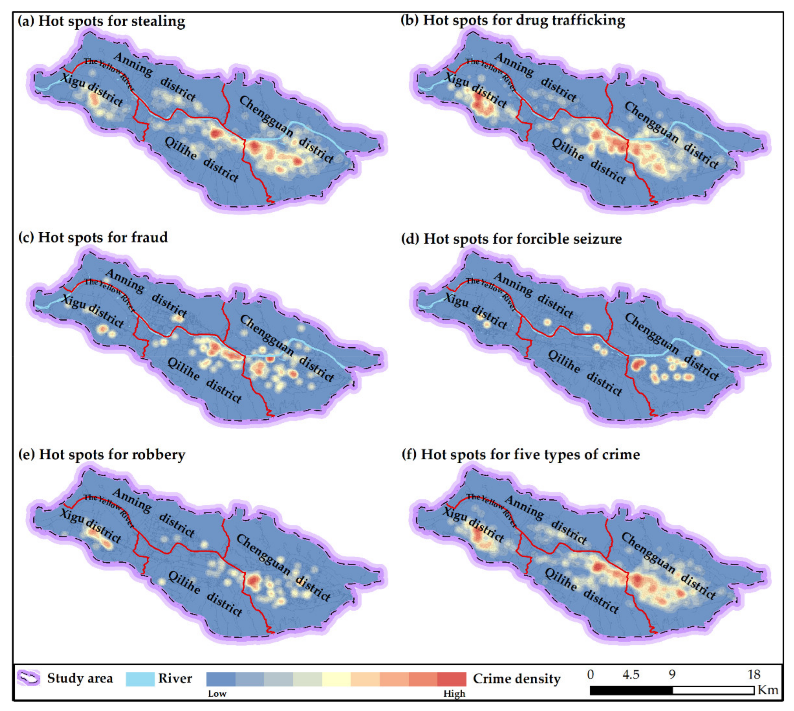
There were 3539 cases of five types of crimes: 1887 cases of stealing, 1405 cases of drug trafficking, 124 cases of fraud, 24 cases of forcible seizure, and 99 cases of robbery. We begin with a spatial autocorrelation analysis of the five types of crime and analyze the spatial aggregation. As shown in Table 10, the result shows that these crimes pass the 99% statistical significance test. The data show that these four crimes (stealing, drug trafficking, fraud, and robbery) share a strong spatial correlation. Their crime rate is related to the area’s location and is clustered and distributed within the urban space, which can be used to identify crime hot spots. We find that Lanzhou crime has characteristic cold and hot spots in the space. However, the location of robbery crimes is random and has no spatial autocorrelation.
To verify the spatial autocorrelation results, we analyze the proximity of different types of crime data in a kernel density space, such as in Figure 11. The geographical spatial distribution map shows that stealing, drug trafficking, fraud, and robbery are mainly concentrated and distributed within the central region of Xigu district, Chengguan district, and Qilihe district. Finally, we obtain the same result as for spatial autocorrelation.
(2)
Potential locations of crime
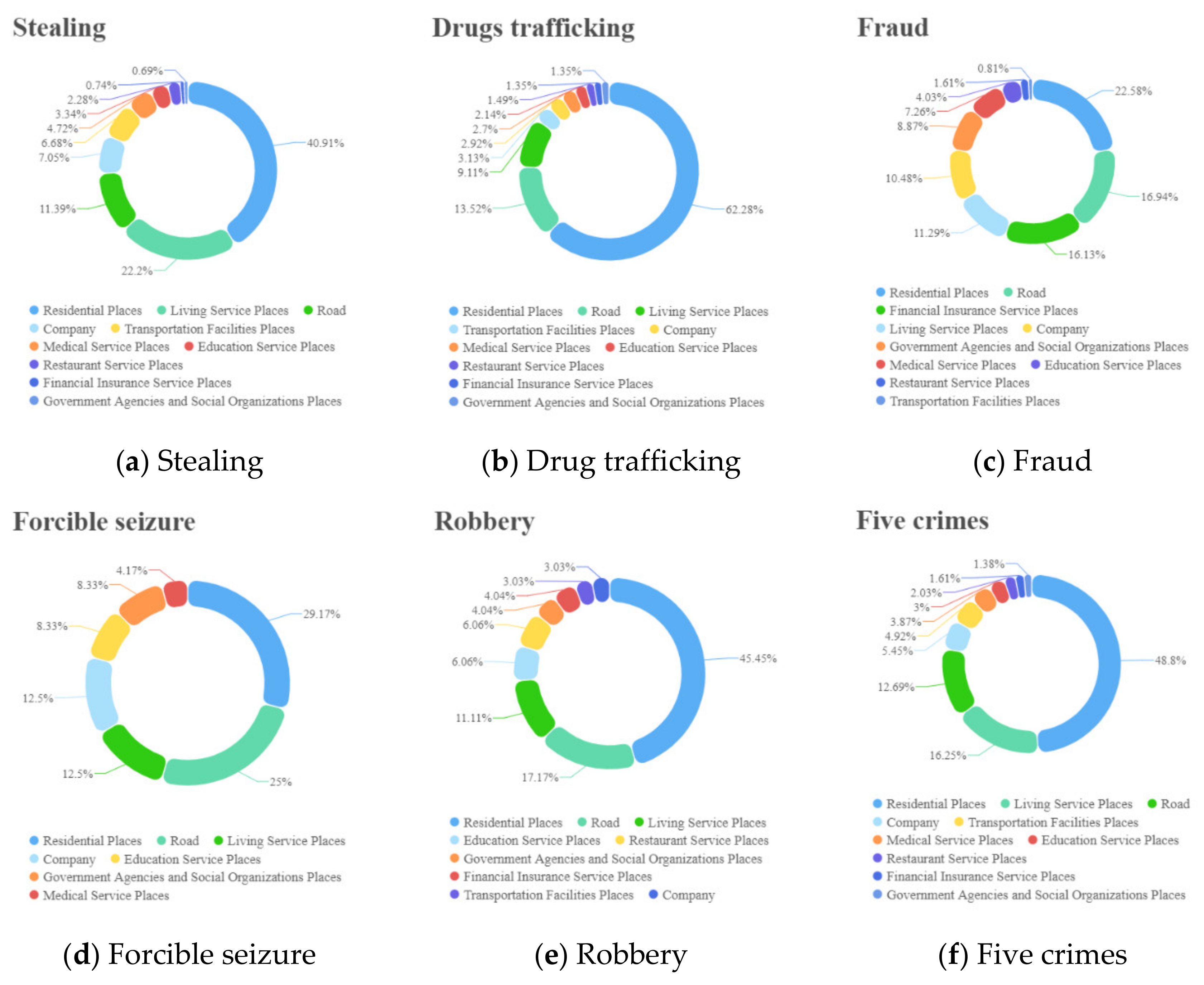
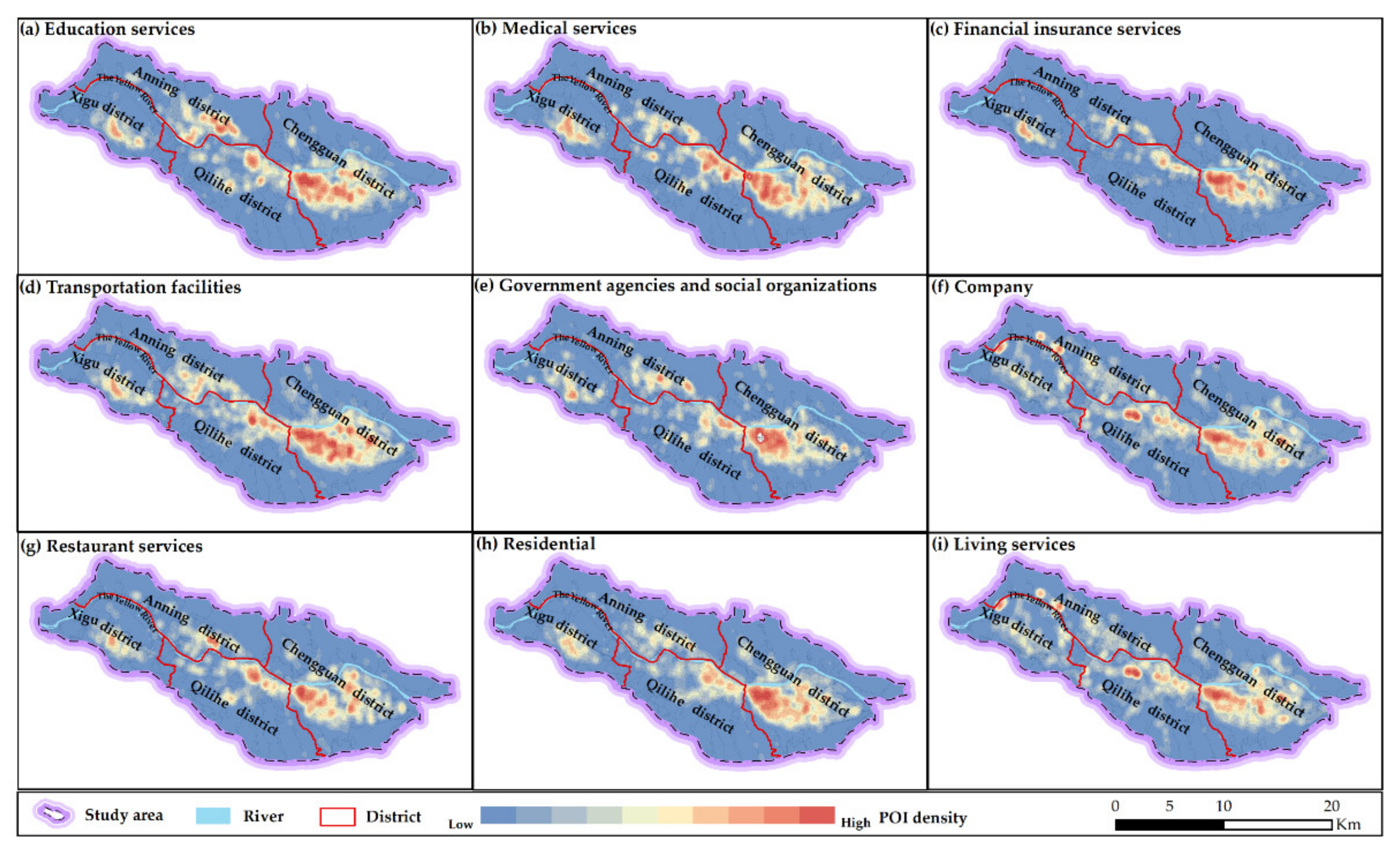
Figure 12 shows a statistical analysis of different types of crime data. Residential areas are the main locations that attract all five types of crime. Living service areas rank second for stealing and third for drug trafficking, forcible seizure, and robbery. Roadside areas rank second for drug trafficking, fraud, forcible seizure, and robbery. Financial insurance service areas rank third for fraud. Finally, for the five types of crime combined, residential areas experience the most, living service areas are second, and roadside areas are third. As shown in Figure 13, the main concentration of 12 types of POI is at the junction of Chengguan District and Qilihe District, which can be known as a potential crime risk in the area.
Table 4 shows different types of POIs (e.g., attribute functions and social activities) classified into nine potential risk areas based on crime characteristics. The distribution of the spatial agglomeration of each type is then obtained by using the kernel density analysis method.

3.2.3. Evaluation Criteria

(1)
Potential crime hotspots. Figure 11f shows the final distribution of crime hotspots. The Chengguan District is the most crime-intensive area and has many residential and commercial areas.
(2)
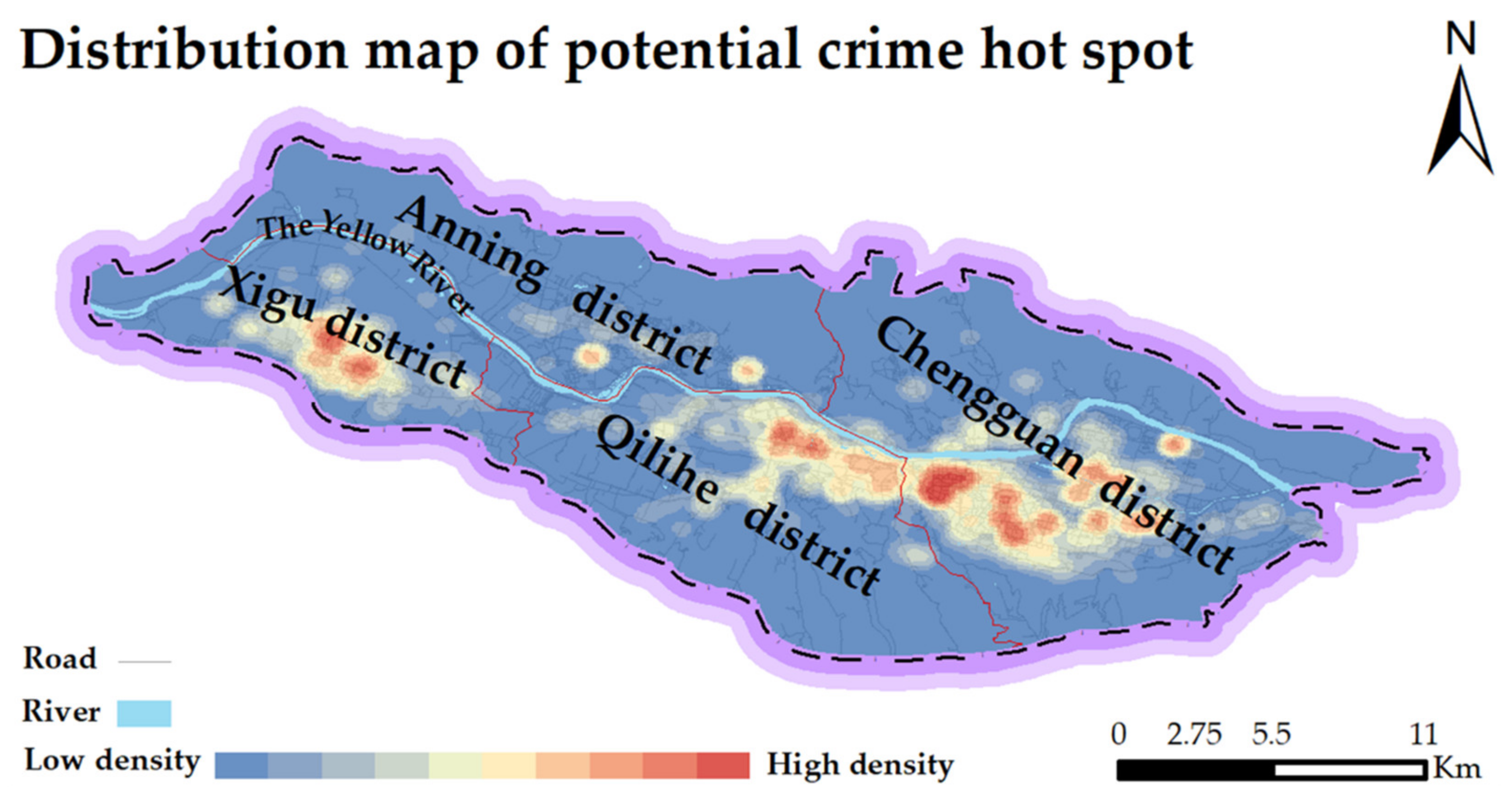
The socioeconomic drivers mainly include population, GDP, proximity to the existing police station, and potential risk areas. The latter are determined by the location where crime occurs (such as attribute functions and social activities) and mainly include education service areas, medical service areas, financial insurance areas, transportation facilities, government agencies and social organizations areas, companies, restaurant service areas, residential areas, and living service areas. The weightings of different POI types are calculated based on the fraction of crime sites, as shown in Table 9. The final potential crime risk map is shown in Figure 14, and its clustering results are similar to the potential crime hotspot map, with the potential occurrence of crime mainly concentrated in the Chengguan district. The accuracy of its results is verified.
(3)
Climatic and environmental driver. (i) Digital elevation model. (ii) Slope. As shown in Figure 7.
Numerous weights are shown in Table 11, and the final consistency ratio is less than 0.1, which indicates that the paired comparison matrix passes the consistency test.
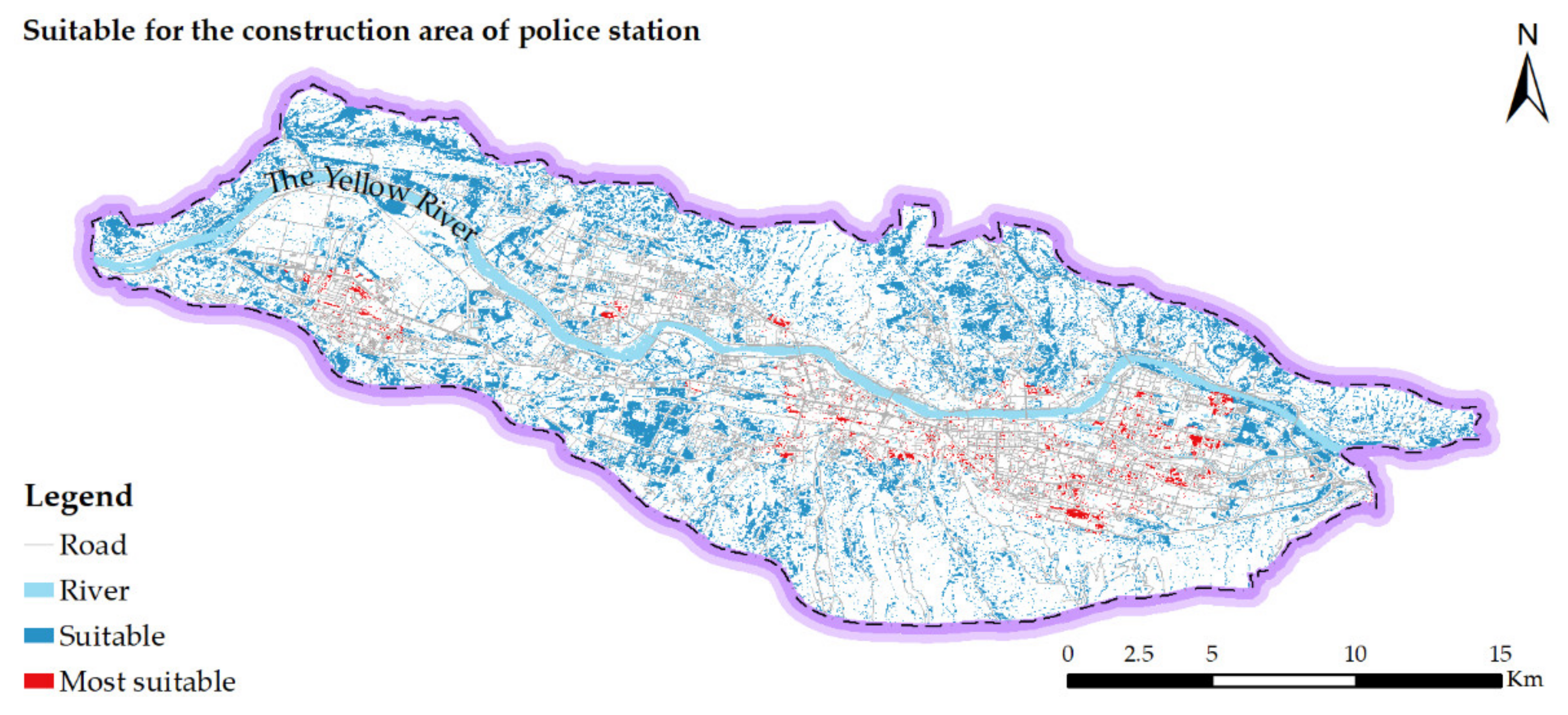
The weighted linear combination method is used to calculate the weighted overlap and obtain the total area for possible police station construction. Figure 15 shows the most suitable areas, the suitable areas, and the unsuitable areas for the police stations. The suitable area for police station construction covers 64.07 km2, which represents 18.67% of the total area. The white area is unsuitable for police station construction. Candidate police stations should first be built in the most suitable areas, following which construction in the suitable areas may be considered.

3.2.4. Coverage of Existing Police Stations

(1)
Current situation
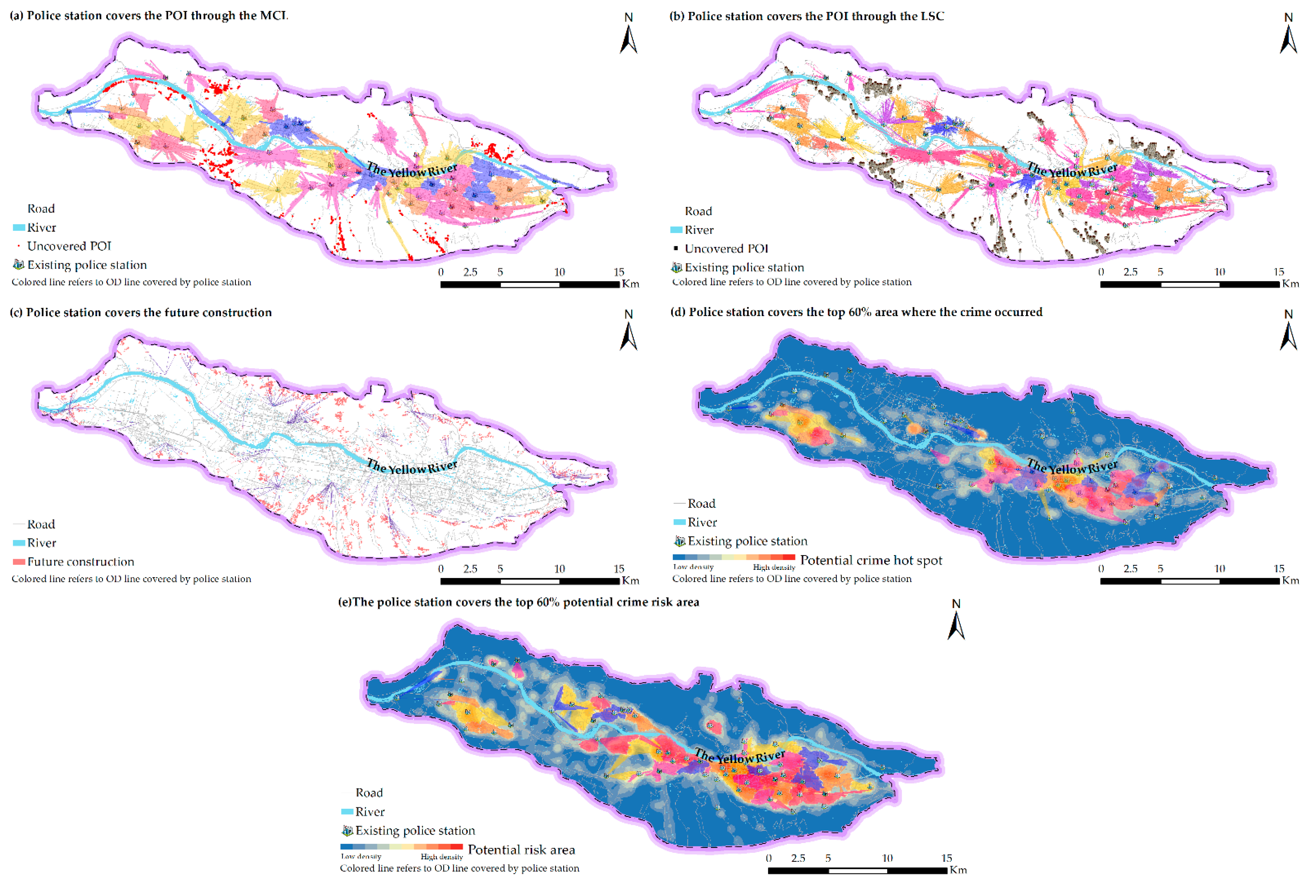
We now present a spatial analysis and optimization of police stations based on the land identified as suitable for such a purpose. According to the spatial layout of urban police stations, the proposed method is applied to spatially analyze the locations of police stations in the central urban area of Lanzhou. The MCL method is used to analyze the coverage provided by 57 existing police stations, with a constant 5 min police response used as a constraint. Using the MCL method to analyze the overall coverage of 62,473 urban POIs, we find that the existing police stations cover 61,202 POIs, which gives a coverage rate of 97.97%. Using the LSC method to analyze the overall coverage of 62,473 urban POIs, we find that the 41 existing police stations cover 61,202 POI points, which gives a coverage of 97.97%. In the central urban area of Lanzhou, the service areas of the police stations overlap significantly in space. An analysis of the spatial distribution of future construction shows that a shortage of police stations will occur mainly in the north and south, which will have an overall coverage of 55.39%. Analysis of the police station coverage of areas where crime is likely to occur shows that the existing police stations cover 100% of the top 60% of crime risk areas, as shown in Figure 16d. Analysis of the police station coverage of high potential crime risk areas shows that the existing police stations cover 100% of the top 60% of the crime risk areas, as shown in Figure 16e.
To summarize, the coverage of existing police stations overlaps significantly in the central urban area of Lanzhou. The areas not covered by the police station service area are mainly distributed in the northern, southern, and northeastern regions. Some POIs and future buildings cannot achieve 100% full coverage given the constraint of a 5 min response time. Therefore, new police stations must be added in these blind areas.
(2)
Prediction of idealized coverage by police stations
The ideal state is to optimize the location of police stations without considering government funds. The idealized state includes mainly the following two scenarios. Scenario 1 does not consider the existing police stations but combines the candidate locations for police stations with spatial location selection and optimization to determine the minimum number of police stations required in the study area. Scenario 2 considers the existing police stations combined with the candidate locations of police stations to increase the police service capacity in areas that are currently under-serviced and determine the maximum number of police stations required in the study area. In Scenario 1, 58 police stations are simulated through four interactions, and in Scenario 2, 89 police stations are simulated through four interactions (see Figure 17).
Although the existing 57 police stations are less than the minimum number of police stations simulated in Scenario 1, it remains a reasonable number. The analysis of the spatial distribution of the police stations shows that they are relatively dense, which can easily lead to problems such as redundancy of police stations. Therefore, given factors such as existing police stations, the area occupied by police stations, the suitable area for the construction of police stations, and the future urban development, we construct a reasonable and scientific layout of police stations that takes into account local conditions.

3.2.5. Spatial Optimization

(1)
Non-overlapping. We filter out redundant police stations in the space. Taking the existing police station as a candidate set and considering road nodes, we consider POIs in important areas and crime points as demand points. The solution is based on the distance of the road network, ensuring the coverage of the existing demand points, eliminating redundant police stations, and maintaining a minimum number of police stations. The results appear in Figure 18. In total, 44 police stations are conserved, and 13 police stations are to be adjusted. According to the density analysis of the proposed (i.e., new) police stations, we conclude that police stations that create more redundancy and service overlap mainly appear in the Chengguan District south of the Yellow River and at the junction of the Qilihe District and the Chengguan District.
(2)
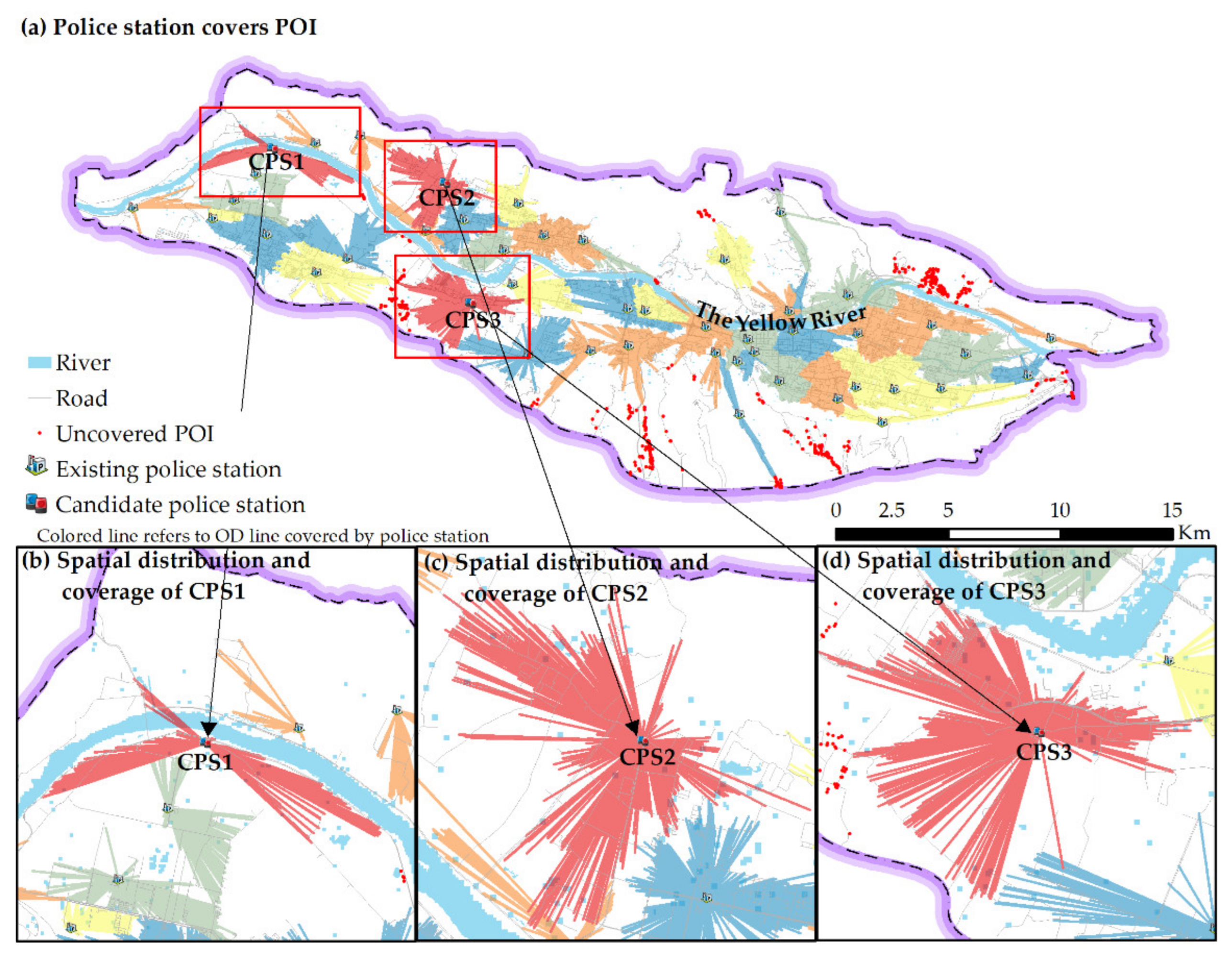
To manage and control key areas, optimize the centralized coverage of key areas and use the filtered POI data of important areas and geocoded crime point data as the demand point set because the global POI data in the central urban area of Lanzhou include all the POI data. Therefore, we select the global POI data in the central urban area of Lanzhou as the demand point set because it is more objective and standardized. Experimentation shows that, when the POI coverage exceeds 99%, the optimization efficiency is minimized, so the key area coverage target at this stage is set to 99%. Based on 44 police stations, 1 of the candidate police stations is selected for re-layout each time. When the number of police stations reaches 47, the POI coverage increases to 99.20%, reaching the established target. Figure 19 shows the spatial distribution of the police stations after the second-stage optimization.
(3)
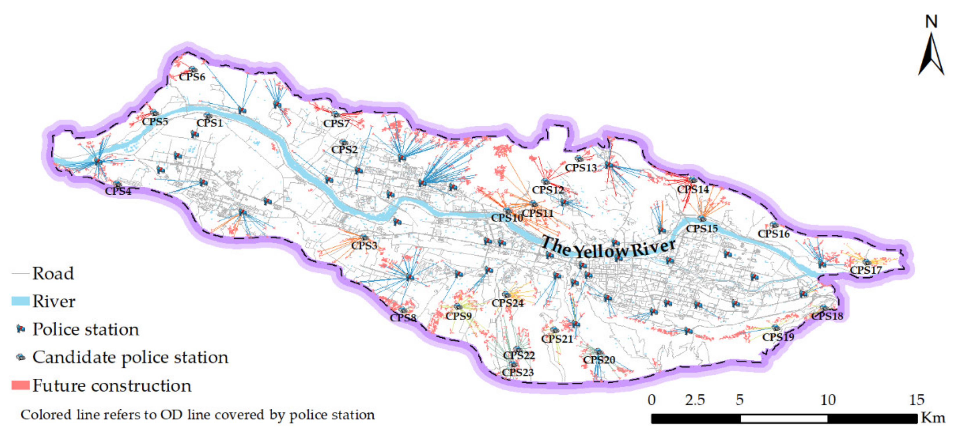
Spatial layout of police stations as a function of future urban changes. We now discuss the layout optimization of candidate police station locations. We spatially adjust 5, 10, 15, and 20 candidate police stations and perform four optimizations. After this optimization, the number of police stations reaches 67, between the minimum number of police stations simulated by Scenario 1 and the maximum number of police stations simulated by Scenario 2. The overall coverage reaches 99%, as shown in Figure 20.

3.3. Distribution of Public Security Police Force and Household Registration Police Force

Based on the optimization of the spatial location of the police stations, we spatially allocate and distribute the public security police force and the household registration police force between the police stations. By aggregating crime point data into street units and studying the spatial distribution of crime in the Lanzhou city center, we find that Lanzhou crime has characteristic cold and hot spots in the space, with the crime hot spots mainly distributed in the areas south of the Yellow River.
By aggregating residential data into street units and studying the spatial distribution of building areas in the central urban area of Lanzhou, we find that the spatial distribution of buildings also reveals spatial differentiation. The spatial heterogeneity of crime and residential buildings in Lanzhou has given rise to differences in the number of public security police force and household registration police force in different police stations.
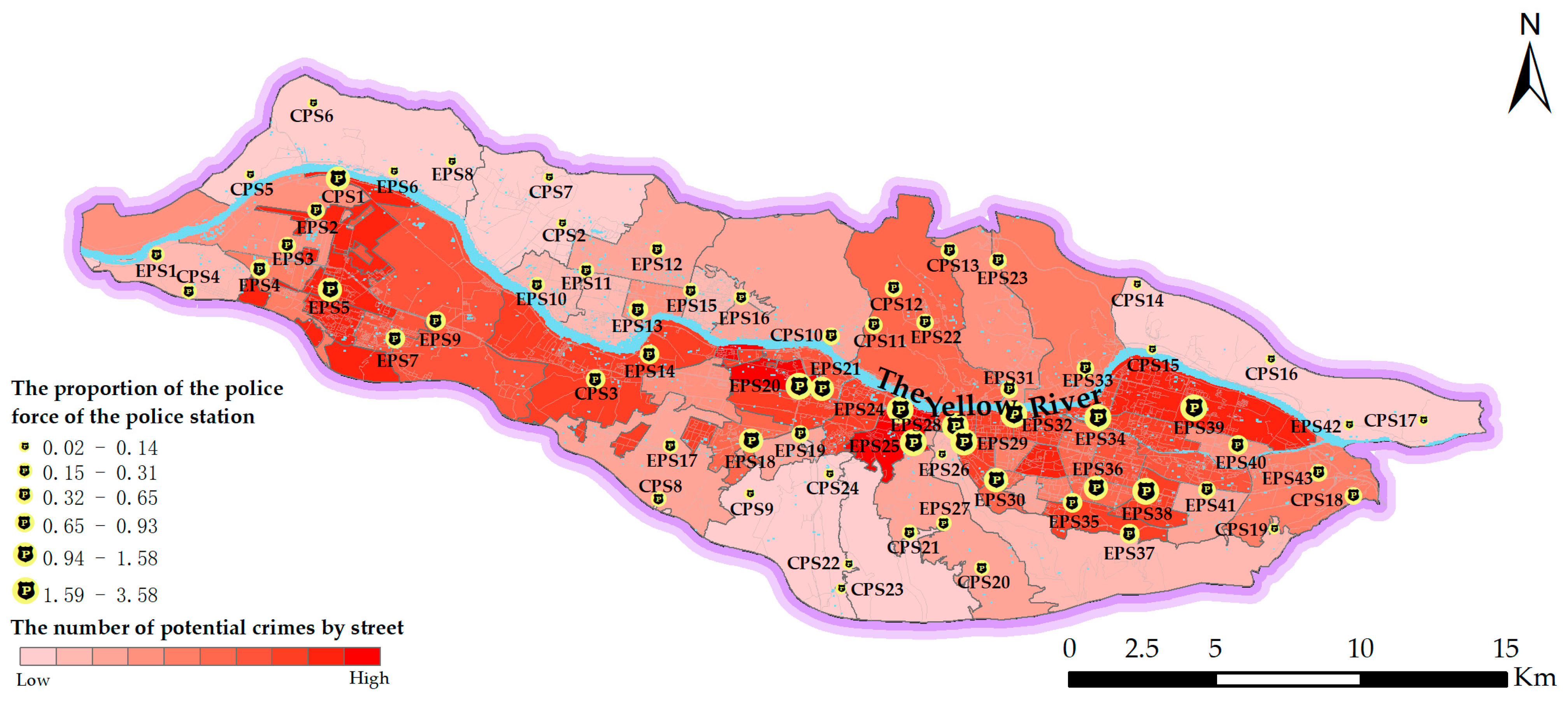
In addition, as shown in Table 12, the ratio of the number of public security police forces to the number of household registration police forces in the same police station also differs between the police stations. This inconsistency reflects the differences in demand for these forces in a given region. The police stations with more public security police forces are mainly concentrated in the central area along the Yellow River, in a belt-like distribution pattern. In contrast, the police stations with more household registration police forces are more scattered, clustered along the Yellow River and in the area east of the Yellow River and west of the south of the Yellow River, as shown in Figure 21 and Figure 22.

4. Discussion

With the rapid growth of China’s population and economy, urban security has become an important topic that many people care about. Therefore, it is very important to reasonably control the deployment of urban police stations. In cities, land use, different functions of POIs, and crime risk profiles tend to vary, so there may be a lack of risk profile assessments, making the deployment of police stations unreasonable. The challenge of preventing disasters from occurring can be daunting for city managers and emergency responders. Lanzhou, one of the largest integrated cities in China, also faces the same urban safety issues as most cities. Due to the limitations of existing buildings in the city, areas not suitable for the construction of police stations are excluded. Furthermore, considering the high timeliness and broad coverage of POI in terms of geography, we demonstrate here the potential and value of POIs in urban risk assessment. At the same time, with the development of the internet technology, spatiotemporal road network data cover most cities. Therefore, the framework of the work presented herein can be transferred to other types of cities.
However, cities are huge, complex, dynamic systems, which may affect the accuracy of crime estimates. First, POI data are abstract points without a building area, building volume, or building shape, and thus cannot reflect the size of a building, which may affect the estimation accuracy of the potential crime area. Second, the distribution of housing buildings as a reflection of the distribution of the population is subject to error because unoccupied buildings or neighborhoods may be concentrated, which can affect the analysis. Therefore, it is necessary to justify it or mention the possibility of adding some other considerations depending on the case study. Third, the method and framework proposed in this paper are implemented in different areas of interest. The impact of different facility locations may require different factors and local characteristics to be considered. For example, a fire station may need to combine water and fire data for site selection. Finally, this work considers many other aspects (geographical, social, economic, people flows, etc.) and thus improves upon the existing methodology. We believe that, with the development of cities, the emergence of new data will further help solve these problems.

5. Conclusions

Predicting future urban changes, analyzing potential crime risks, and determining the location of police stations are important tasks to improve urban management and reduce crime. This paper presents the results of different chronological land type classifications, predictions of urban change, and assessments of site suitability for hosting police stations. According to urban risk assessment methods and existing norms, POI data are divided into different risk areas, standardized, and weighted with the help of the analytic hierarchy process model. The distribution of risk areas is determined by superposition. Based on the existing police stations, the construction of a new police station is triggered only after comprehensively considering its impact on the POI and the overall building construction area, and after optimizing the spatial configuration of all police stations. The overall goal is to improve service and shorten police response time. A further consideration is given to spatial differences in public security police forces and household registration police forces. The main conclusions are as follows:
(1)
Data analysis shows that crime is mainly concentrated in densely populated areas, indicating that people and wealth are the main motives driving crime. Theft is the most common of the five crime types. Urban expansion gradually spreads to the periphery, and the city’s interior is constantly filled, among which the northern part of Anning District becomes more developed. Differences in the spatial distribution of crime hotspots and construction result in a spatially heterogenous ratio of the public security police forces to household registration police forces allocated to the different police stations.
(2)
Coverage analysis indicates that the overall coverage of POIs by existing police stations is 97.97%, and the comprehensive coverage predicted for future land use falls to 55.39%. The method proposed herein reduces the overlap of police station service areas (22.8%), increases area coverage (12.01%) and demand point coverage (7.25%), removes 13 existing police stations, and adds 24 candidate police stations. This method combines the point of view of big data with novel ideas and a technical scheme for selecting sites for police stations.

Author Contributions

Conceptualization, Yuncheng Jiang and Zhigang Yan; methodology, Yuncheng Jiang and Zhigang Yan; software, Zhigang Yan and Baoyu Guo; validation, Zhigang Yan and Baoyu Guo; formal analysis, Yuncheng Jiang; investigation, Zhigang Yan; resources, Yuncheng Jiang; data curation, Yuncheng Jiang; writing—original draft preparation, Yuncheng Jiang; writing—review and editing, Yuncheng Jiang, Zhigang Yan and Baoyu Guo; visualization, Yuncheng Jiang; supervision, Zhigang Yan and Baoyu Guo; project administration, Zhigang Yan; funding acquisition, Zhigang Yan and Baoyu Guo. All authors have read and agreed to the published version of the manuscript.

Funding

This research was funded in part by the National Natural Science Foundation of China (No. 41971370).

Institutional Review Board Statement

Not applicable.

Informed Consent Statement

Not applicable.

Data Availability Statement

The data used in this study are available from the corresponding author upon reasonable request.

Acknowledgments

The authors would like to thank the anonymous reviewers for their helpful and valuable comments and suggestions.

Conflicts of Interest

The authors declare no conflict of interest.

References

  1. Jiang, Y.C.; Lv, A.F.; Yan, Z.G.; Yang, Z. A GIS-Based Multi-Criterion Decision-Making Method to Select City Fire Brigade: A Case Study of Wuhan, China. ISPRS Int. J. Geo-Inf. 2021, 10, 777. [Google Scholar] [CrossRef]
  2. Xue, D.S.; Zeng, X.J. Evaluation of China’s urbanization quality and analysis of its spatial pattern transformation based on the modern life index. Acta Geogr. Sin. 2016, 71, 194–204. [Google Scholar] [CrossRef]
  3. Wang, F.Z. Necessity and method of location allocation for urban public security agencies. Urban Probl. 1995, 1, 11–14. [Google Scholar] [CrossRef]
  4. Hakimi, S.L. Optimum distribution of switching centers in a communication network and some related graph theoretic problems. Oper. Res. 1965, 13, 462–475. [Google Scholar] [CrossRef]
  5. Church, R.L. The regionally constrained p–median problem. Geogr. Anal. 1990, 22, 22–32. [Google Scholar] [CrossRef]
  6. Murray, A.T.; Gerrard, R.A. Capacitated service and regional constraints in location-allocation modeling. Locat. Sci. 1997, 5, 103–118. [Google Scholar] [CrossRef]
  7. Gong, D.; Gen, M.; Yamazaki, G.; Xu, W. Hybrid evolutionary method for capacitated location-allocation problem. Comput. Ind. Eng. 1997, 33, 577–580. [Google Scholar] [CrossRef]
  8. Marianov, V.; Serra, D. Hierarchical location–allocation models for congested systems. Eur. J. Oper. Res. 2001, 135, 195–208. [Google Scholar] [CrossRef] [Green Version]
  9. Lozano, S.; Guerrero, F.; Onieva, L.; Larrañeta, J. Kohonen maps for solving a class of location-allocation problems. Eur. J. Oper. Res. 1998, 108, 106–117. [Google Scholar] [CrossRef]
  10. Salhi, S.; Gamal, M.D. A genetic algorithm based approach for the uncapacitated continuous location–allocation problem. Ann. Oper. Res. 2003, 123, 203–222. [Google Scholar] [CrossRef]
  11. Hsieh, K.H.; Tien, F.C. Self-organizing feature maps for solving location–allocation problems with rectilinear distances. Comput. Oper. Res. 2004, 31, 1017–1031. [Google Scholar] [CrossRef]
  12. Li, X.; Ye, J.A. Optimal Spatial Search Using Genetic Algorithms and GIS. Acta Geogr. Sin. 2004, 59, 745–753. [Google Scholar] [CrossRef]
  13. Liang, Q.O. Researches on Obstacle Location-allocation Problem Based on Clonal Selection Principle. Geomat. Inf. Sci. Wuhan Univ. 2007, 32, 744–747. [Google Scholar]
  14. Gang, Z. Urban fire risk evaluation and its application based on spatial analysis: A case study of Xi’an. City Plan. Rev. 2016, 40, 59–64. [Google Scholar] [CrossRef]
  15. Wang, W.; Xu, Z.; Sun, D.; Lan, T. Spatial optimization of mega-city fire stations based on multi-source geospatial data: A case study in Beijing. ISPRS Int. J. Geo-Inf. 2021, 10, 282. [Google Scholar] [CrossRef]
  16. Yuan, F.; Wei, Y.H.; Chen, W.; Jin, Z. Spatial agglomeration and new firm formation in the information and communication technology industry in suzhou. Acta Geogr. Sin. 2010, 65, 153–163. [Google Scholar] [CrossRef]
  17. Zha, A.P.; Xu, N.; Hou, Z.G. A study on the suitability of the micro location of Eco Hotel. Hum. Geogr. 2017, 32, 152–160. [Google Scholar]
  18. Martín-Fernández, S.; Martínez-Falero, E.; Peribáñez, J.R.; Ezquerra, A. GIS-Based Simulated Annealing Algorithm for the Optimum Location of Fire Stations in the Madrid Region, Spain: Monitoring the Collapse Index. Appl. Sci. 2021, 11, 8414. [Google Scholar] [CrossRef]
  19. Chen, C.; Ren, A.Z. Optimization of fire station locations using computer. Qinghua Daxue Xuebao/J. Tsinghua Univ. (China) 2003, 43, 1390–1393. [Google Scholar]
  20. Chen, H. Study on Optimization of the Spatial Distribution of City Fire Station in Lu’an City. Master’s Thesis, Tongji University, Shanghai, China, 2007. [Google Scholar] [CrossRef]
  21. Zhang, T.; Ma, S.; Shen, H. Equity-Oriented Time -Varying Emergency Management Service Coverage Optimization. Geomat. Inf. Sci. Wuhan Univ. 2017, 42, 1681–1687. [Google Scholar] [CrossRef]
  22. Song, Z.N.; Yan, T.G.; Liu, T.; Huang, T. A new gravity P-median model and empirical test in urban comprehensive hospital location decision making: Take Wuxi as an example. Prog. Geogr. 2016, 35, 420–430. [Google Scholar] [CrossRef] [Green Version]
  23. Xie, X.H.; Wang, R.Z.; Wen, D.H.; Zhang, Z.Y. Evaluating the medical facilities layout based on gis: An application of Xiang’an district. J. Geo-Inf. Sci. 2015, 17, 317–328. [Google Scholar] [CrossRef]
  24. Peng, Y.; Wang, Z. Space operation of rural primary and secondary school location. Acta Geogr. Sin. 2013, 68, 1411–1417. [Google Scholar] [CrossRef]
  25. Dai, T.; Liao, C.; Hu, K.; Zhang, W.; Liu, Z. Secondary school allocation optimization towards equal access: A case study on Shijingshan District, Beijing. Acta Geogr. Sin. 2017, 72, 1476–1485. [Google Scholar] [CrossRef]
  26. Kong, Y.; Zhu, Y.; Wang, Y. A hybrid metaheuristic algorithm for the school districting problem. Acta Geogr. Sin. 2017, 72, 256–268. [Google Scholar] [CrossRef]
  27. Li, S.; Du, Q. Suitability of Regional Multi-airports Planning by Hierarchical P-median Location Model. Geomat. Inf. Sci. Wuhan Univ. 2012, 37, 988–991. [Google Scholar]
  28. Zou, Y.; Liu, Y.; Kong, X.; Fan, D. Optimization of Rural Residential Land Based on Weighted-Voronoi Diagram. Geomat. Inf. Sci. Wuhan Univ. 2012, 37, 560–563. [Google Scholar]
  29. Tang, C.L.; He, Y.; Zhou, G.; Zeng, S.S.; Xiao, L.Y. The research on optimization mode of spatial organization of rural settlements oriented by life quality. Acta Geogr. Sin. 2014, 69, 1459–1472. [Google Scholar] [CrossRef]
  30. Ding, J.; Jin, F.; Wang, C.; Wang, J. Evaluation, Optimization and Simulation of the Spatial Layout of Transport Hubs in China. Acta Geogr. Sin. 2011, 66, 504–514. [Google Scholar] [CrossRef]
  31. Xu, W.; Ma, Y.; Zhao, X.; Li, Y.; Qin, L.; Du, J. A comparison of scenario-based hybrid bilevel and multi-objective location-allocation models for earthquake emergency shelters: A case study in the central area of Beijing, China. Int. J. Geogr. Inf. Sci. 2018, 32, 236–256. [Google Scholar] [CrossRef]
  32. Zhao, R.; Yang, L.; Shao, J. A Method for Multi-constraint Location Decision of Distribution Center Based on Refined Ant Colony Algorithm and GIS. J. Geo-Inf. Sci. 2015, 17, 172–177. [Google Scholar] [CrossRef]
  33. Du, W.; Li, Q.S. Economic analysis on transportation delaminating in distribution System. Syst. Eng. Theory Pract. 2003, 4, 82–85. [Google Scholar]
  34. Curtin, K.M.; Hayslett-Mccall, K.; Qiu, F. Determining optimal police patrol areas with maximal covering and backup covering location models. Netw. Spat. Econ. 2010, 10, 125–145. [Google Scholar] [CrossRef]
  35. Adler, N.; Hakkert, A.S.; Kornbluth, J.; Raviv, T.; Sher, M. Location-allocation models for traffic police patrol vehicles on an interurban network. Annals of Operations Research. 2014, 221, 9–31. [Google Scholar] [CrossRef]
  36. Dunnett, S.; Leigh, J.; Jackson, L. Optimising police dispatch for incident response in real time. J. Oper. Res. Soc. 2019, 70, 269–279. [Google Scholar] [CrossRef] [Green Version]
  37. Milias, V.; Psyllidis, A. Assessing the influence of point-of-interest features on the classification of place categories. Comput. Environ. Urban Syst. 2021, 86, 101597. [Google Scholar] [CrossRef]
  38. Martí, P.; Serrano-Estrada, L.; Nolasco-Cirugeda, A. Social media data: Challenges, opportunities and limitations in urban studies. Comput. Environ. Urban Syst. 2019, 74, 161–174. [Google Scholar] [CrossRef]
  39. Xiong, X.; Qiao, S.; Li, Y.; Han, N.; Yuan, G.; Zhang, Y. A point-of-interest suggestion algorithm in Multi-source geo-social net-works. Eng. Appl. Artif. Intell. 2020, 88, 103374. [Google Scholar] [CrossRef]
  40. Yao, Y.; Li, X.; Liu, X.; Liu, P.; Liang, Z.; Zhang, J.; Mai, K. Sensing spatial distribution of urban land use by integrating points-of-interest and Google Word2Vec model. Int. J. Geogr. Inf. Sci. 2017, 31, 825–848. [Google Scholar] [CrossRef]
  41. McKenzie, G.; Janowicz, K. Where is also about time: A location-distortion model to improve reverse geocoding using behavior-driven temporal semantic signatures. Comput. Environ. Urban Syst. 2015, 54, 1–13. [Google Scholar] [CrossRef]
  42. Ding, H.; Shi, W. Land-use/land-cover change and its influence on surface temperature: A case study in Beijing City. Int. J. Remote Sens. 2013, 34, 5503–5517. [Google Scholar] [CrossRef]
  43. Jiang, J.; Tian, G. Analysis of the impact of land use/land cover change on land surface temperature with remote sensing. Procedia Environ. Sci. 2010, 2, 571–575. [Google Scholar] [CrossRef] [Green Version]
  44. Sang, X.; Guo, Q.; Wu, X.; Fu, Y.; Xie, T.; He, C.; Zang, J. Intensity and stationarity analysis of land use change based on CART algorithm. Sci. Rep. 2019, 9, 12279. [Google Scholar] [CrossRef] [PubMed] [Green Version]
  45. Liang, X.; Guan, Q.; Clarke, K.C.; Liu, S.; Wang, B.; Yao, Y. Understanding the drivers of sustainable land expansion using a patch-generating land use simulation (PLUS) model: A case study in Wuhan, China. Comput. Environ. Urban Syst. 2021, 85, 101569. [Google Scholar] [CrossRef]
  46. He, Z.; Deng, M.; Cai, J.; Xie, Z.; Guan, Q.; Yang, C. Mining spatiotemporal association patterns from complex geographic phenomena. Int. J. Geogr. Inf. Sci. 2020, 34, 1162–1187. [Google Scholar] [CrossRef]
  47. Liu, Y.; Liu, Y.; Chen, Y.; Long, H. The process and driving forces of rural hollowing in China under rapid urbanization. J. Geogr. Sci. 2010, 20, 876–888. [Google Scholar] [CrossRef]
  48. Lee, S.W.; Hwang, S.J.; Lee, S.B.; Hwang, H.S.; Sung, H.C. Landscape ecological approach to the relationships of land use patterns in watersheds to water quality characteristics. Landsc. Urban Plann. 2009, 92, 80–89. [Google Scholar] [CrossRef]
  49. Tan, M.; Li, X. The changing settlements in rural areas under urban pressure in China: Patterns, driving forces and policy implications. Landsc. Urban Plann. 2013, 120, 170–177. [Google Scholar] [CrossRef]
  50. Thorsen, I.; Ubøe, J. Modelling residential location choice in an area with spatial barriers. Ann. Reg. Sci. 2002, 36, 613–644. [Google Scholar] [CrossRef]
  51. Long, Y.; Han, H.; Lai, S.; Mao, Q. Urban growth boundaries of the Beijing metropolitan area: Comparison of simulation and artwork. Cities 2013, 31, 337–348. [Google Scholar] [CrossRef]
  52. Geary, R.C. The Contiguity Ratio and Statistical Mapping. Inc. Stat. 1954, 5, 115–146. [Google Scholar] [CrossRef]
  53. Goodchild, M.; Haining, R.; Wise, S. Integrating Gis and Spatial Data Analysis: Problems and Possibilities. Int. J. Geogr. Inf. Syst. 1992, 6, 407–423. [Google Scholar] [CrossRef]
  54. Moran, P.A.P. The Interpretation of Statistical Maps. J. R. Stat. Soc. Ser. A Stat. Soc. 1948, 10, 243–251. [Google Scholar] [CrossRef]
  55. De FSM Russo, R.; Camanho, R. Criteria in AHP: A systematic review of literature. Procedia Comput. Sci. 2015, 55, 1123–1132. [Google Scholar] [CrossRef] [Green Version]
  56. Dožić, S.; Kalić, M. Comparison of two MCDM methodologies in aircraft type selection problem. Transp. Res. Procedia 2015, 10, 910–919. [Google Scholar] [CrossRef] [Green Version]
  57. Höfer, T.; Sunak, Y.; Siddique, H.; Madlener, R. Wind farm siting using a spatial Analytic Hierarchy Process approach: A case study of the Städteregion Aachen. Appl. Energy 2016, 163, 222–243. [Google Scholar] [CrossRef]
  58. Rinner, C.; Voss, S. MCDA4ArcMap—An open-source multi-criteria decision analysis and geovisualization tool for ArcGIS 10. Feature Artic. Cart. Newsl. Can. Cartogr. Assoc. 2013, 15, 101–127. [Google Scholar]
  59. Pinar, A.O.; Yasin, E.M.; Ertugrul, C.; Cam, E.; Inanc, N. Optimal site selection for a solar power plant in the central anatolian region of Turkey. Int. J. Photoenergy 2017, 2017, 7452715. [Google Scholar] [CrossRef] [Green Version]
  60. Chakraborty, S.; Banik, D. Design of a material handling equipment selection model using analytic hierarchy process. Int. J. Adv. Manuf. Technol. 2006, 28, 1237–1245. [Google Scholar] [CrossRef]
  61. Cooper, L. Location-allocation problems. Oper. Res. 1963, 11, 331–343. [Google Scholar] [CrossRef]
  62. Menezes, R.C.; Pizzolato, N.D. Locating public schools in fast expanding areas: Application of the capacitated p-median and max-imal covering location models. Pesqui. Oper. 2014, 34, 301–317. [Google Scholar] [CrossRef] [Green Version]
  63. Zarrinpoor, N.; Fallahnezhad, M.S.; Pishvaee, M.S. Design of a reliable hierarchical location-allocation model under disruptions for health service networks: A two-stage robust approach. Comput. Ind. Eng. 2017, 109, 130–150. [Google Scholar] [CrossRef]
  64. Rahman, M.; Chen, N.; Islam, M.; Dewan, A.; Pourghasemi, H.R.; Washakh, R.M.A.; Nepal, N.; Tian, S.; Faiz, H.; Alam, M.; et al. Location-allocation modeling for emergency evacuation planning with GIS and remote sensing: A case study of Northeast Bangladesh. Geosci. Front. 2021, 12, 101095. [Google Scholar] [CrossRef]
  65. Murray, A.T. Optimizing the spatial location of urban fire stations. Fire Saf. J. 2013, 62, 64–71. [Google Scholar] [CrossRef]
  66. Helly, W. Urban Systems Models; Academic Press: Cambridge, MA, USA, 1975. [Google Scholar] [CrossRef]
  67. Plane, D.R.; Thomas, E.; Hendrick, T.E. Mathematical programming and the location of fire companies for the Denver fire de-partment. Oper. Res. 1977, 25, 563–578. [Google Scholar] [CrossRef]
  68. Chaudhary, P.; Chhetri, S.K.; Joshi, K.M.; Shrestha, B.M.; Kayastha, P. Application of an Analytic Hierarchy Process (AHP) in the GIS interface for suitable fire site selection: A case study from Kathmandu Metropolitan city, Nepal. Socio-Econ. Plan. Sci. 2016, 53, 60–71. [Google Scholar] [CrossRef]
  69. Nalepa, J.; Kawulok, M. Selecting training sets for support vector machines: A review. Artif. Intell. Rev. 2019, 52, 857–900. [Google Scholar] [CrossRef] [Green Version]
  70. Gong, B.; Im, J.; Mountrakis, G. An artificial immune network approach to multi-sensor land use/land cover classification. Remote Sens. Environ. 2011, 115, 600–614. [Google Scholar] [CrossRef]
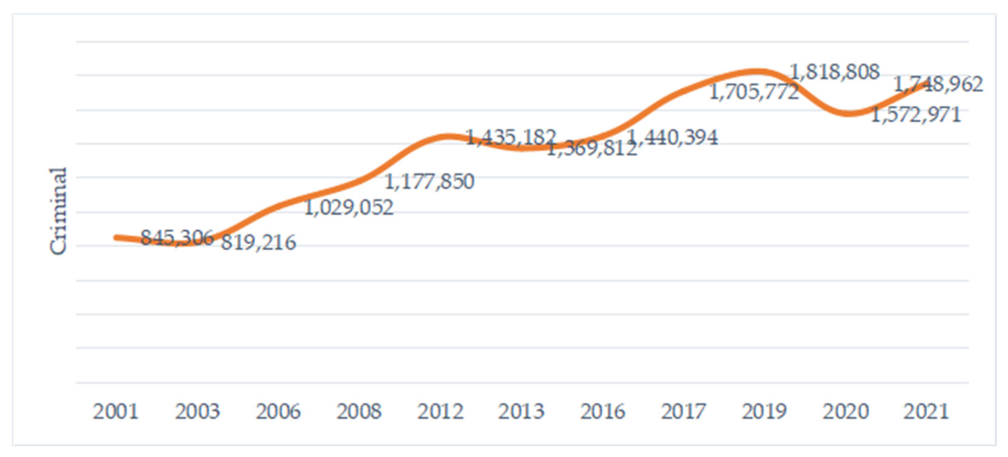
Figure 1. Number of criminal offenses in China prosecuted from 2001 to 2021.
Ijgi 11 00384 g001
Figure 2. Case study area showing central urban area of Lanzhou, China. (a) Geospatial distribution of the study area in China, (b) topography of Lanzhou, and (c) urban landscape of the study area.
Ijgi 11 00384 g002
Figure 3. Flow chart of proposed method for selecting police station locations.
Ijgi 11 00384 g003
Figure 4. Flow chart of land expansion strategy.
Ijgi 11 00384 g004
Figure 5. Distribution of land use. (a) Spatial distribution of land use in 2018. (b) Spatial distribution of land use in 2019. (c) Spatial distribution of land use in 2020. (d) Land use change from 2018 to 2020.
Ijgi 11 00384 g005
Figure 6. Changes in land use. (a) Types of land use areas in 2018–2020. (b) Changes in land use from 2018 to 2019 and from 2019 to 2020.
Ijgi 11 00384 g006
Figure 7. Twelve potential drivers of land use development.
Ijgi 11 00384 g007
Figure 8. The contribution of each variable to the growth of the seven land use types. The most important factors overlap with the expansion of the corresponding land uses.
Ijgi 11 00384 g008
Figure 9. Land use in 2030 based on simulation from 2020.
Ijgi 11 00384 g009
Figure 10. Constraint layer of Lanzhou’s central city.
Ijgi 11 00384 g010
Figure 11. Spatial distribution of crime hot spots.
Ijgi 11 00384 g011
Figure 12. Statistical analysis of crime characteristics.
Ijgi 11 00384 g012
Figure 13. Distribution of kernel density in different potential risk areas.
Ijgi 11 00384 g013
Figure 14. Distribution of potential crime hot spots.
Ijgi 11 00384 g014
Figure 15. “Most suitable” and “suitable” areas for the construction of police stations.
Ijgi 11 00384 g015
Figure 16. Spatial distribution of proximity of existing police stations to crime risk areas. (a) Existing police stations cover the spatial distribution of POIs. (b) Spatial distribution of future construction covered by the existing police stations. (c) Spatial distribution of the top 60% crime hot spots covered by existing police stations. (d) Spatial distribution of the top 60% crime risk area covered by existing police stations. (e) Spatial distribution of the top 60% potential risk area covered by existing police stations.
Ijgi 11 00384 g016
Figure 17. Minimum facilities coverage problem for the existing police station in idealized case.
Ijgi 11 00384 g017
Figure 18. Spatial distribution of redundant police stations.
Ijgi 11 00384 g018
Figure 19. For experiment (1), the spatial distribution of three new candidate police stations in all building contribution sites.
Ijgi 11 00384 g019
Figure 20. For experiment (2), the future spatial distribution of new police stations.
Ijgi 11 00384 g020
Figure 21. Number of street crimes and fraction of public security police force.
Ijgi 11 00384 g021
Figure 22. Street construction area and fraction of household registration police force.
Ijgi 11 00384 g022
Table 1. Seven types of land use classifications.
TypesAbbreviationDescription
ForestryFOTrees in the landscape can be observed from the images. Parcels are planted with fruit trees or shrubs: single or mixed fruit species, fruit trees related to the surface of permanent grassland, etc.
ShrublandSLShrub cover can be identified in the images. The texture is finer than the canopy but coarser than the grasslands, etc.
GrasslandGLGrazing grassland and natural park, etc.
CroplandCLRice cultivation, arable and tillage lands, greenhouse farming, etc.
ConstructionCSUrban and built-up areas, roads, etc.
BarrenBABare soil, wastelands, exposed rock, etc.
WaterbodyWBRiver, lake, pond, canal, dam, ditch, stream, weir, etc.
Table 2. Data for land use development potential drivers.
Main ClassSub-ClassYearOriginal ResolutionData Resource
Land useLand use2018–202030 mGEE
Socioeconomic driverPopulation20151000 mhttp://www.geodoi.ac.cn/WebCn/Default.aspx, (accessed on 29 September 2021).
GDP
Proximity to government202130 mhttps://lbsyun.baidu.com/, (accessed on 29 September 2021).
Proximity to road202130 mOSM
Proximity to railway
Proximity to train station
Climatic and environment driverSoil type20151000 mhttp://www.geodoi.ac.cn/WebCn/Default.aspx, (accessed on 29 September 2021).
Proximity to river202130 mOSM
Annual mean temperature1994–201830 mhttps://www.esmap.org/re_mapping, (accessed on 11 June 2020).
Annual precipitation
DEM201630 mNASA SRTM1 v3.0
Slope
Table 3. Transition matrix and weight of the neighborhood in the natural growth scenario.
Land UseForestryShrublandGrasslandCroplandConstructionBarrenWaterbody
Forestry1000000
Shrubland1111111
Grassland1111111
Cropland0001000
Construction0110110
Barren1111111
Waterbody0000001
Table 4. Rating scale of AHP method.
Numerical ScaleDefinition (i with Respect to j)Value
aijaji
1Equal importance11
3Moderate importance31/3
5Strong importance51/5
7Very strong importance71/7
9Extreme importance91/9
2, 4, 6, 8Intermediate values2, 4, 6, 81/2, 1/4, 1/6, 1/8
Table 5. Random consistency index.
n12345678910
RI000.580.901.121.241.321.411.451.49
Table 6. POI data classification.
Main ClassSubclasses
CompanyConstruction companies, factories, home appliance and electronics stores, pharmaceutical companies, mechanical services, etc.
Restaurant ServicesChinese restaurants, dessert shops, casual dining places, fast food restaurants, cold drink shops, coffee shops, tea houses, etc.
ResidentialResidential homes, buildings, hotels, villages, apartments, travel agencies, bars, etc.
Living ServicesVegetable markets, shopping centers, pedestrian streets, temporary work agencies, post offices, theatres, etc.
Education ServicesElementary school, junior high school, high school, preschool, etc.
Financial Insurance ServicesBanking, insurance, securities trading, etc.
Medical ServicesPharmacies, hospitals, clinics, service stations, etc.
Transportation FacilitiesParking stations, docks, parking lots, etc.
Government Agencies and Social
Organizations
Sports bureaus, government bureaus, public security bureaus, highway bureaus, etc.
Table 7. Mathematical expressions for both L-A algorithms.
Maximize Coverage Location (MCL)Minimize Facilities Coverage (LSC)
Objective function Maximize i a i y i Minimize j J c j x j
Subject to i a i y i y i i
i x j = p
x j = 0 , 1 , j
y j = 0 , 1 , j
j J x j 1 , j J
x j = 0 , 1 , j J
Table 8. Sample number and areas of each land use type.
Land Use TypePointsPolygons2018 (km2)2019 (km2)2020 (km2)
Construction284328181.12185.75187.17
Cropland1333514.4520.4322.92
Barren2768744.2643.9836.17
Forestry1315611.3412.0512.50
Grassland24710680.8670.3173.46
Shrubland620.050.200.28
Waterbody1102510.9210.2810.49
Overall accuracy (%)93.6593.0392.89
Kappa accuracy (%)87.7986.7786.18
Table 9. Contributions to the net change in all land use.
Units: km2ConstructionCroplandBarrenForestryGrasslandShrublandWaterbody
Construction+2.42−4.93+1.08−4.54+0.07−0.16
Cropland−2.39−2.39−0.68−2.83+0.03−0.19
Barren+4.90+2.40+1.16−0.35+0.05−0.04
Forestry−1.04+0.66−1.13+0.44+0.03−0.06
Grassland+4.49+2.83+0.35−0.45+0.10+0.03
Shrubland−0.05−0.03−0.03−0.02−0.08−0.01
Waterbody+0.16+0.19+0.04+0.07−0.04+0.01
Losses−26.08−9.86−31.75−7.40−24.95−0.00−2.23
Gains+32.13+18.33+23.66+8.56+17.55+0.23+1.80
Table 10. Spatial autocorrelation report.
CrimeMoran’s IndexZ Scorep Value
Stealing0.03715527.8730020Clustered
Drug trafficking0.03100123.1162560Clustered
Fraud0.0031692.4517060.014218Clustered
Forcible seizure−0.0001740.1271550.898818Random
Robbery0.0046273.5127710.000443Clustered
Five types of crime0.04417333.0113790Clustered
Table 11. Weightings of all evaluation criteria as determined by the analytic hierarchy process.
CriteriaWeightSub-CriteriaWeight WeightFinal Weight
Potential crime hot spot64.8% 64.8%
Socioeconomic23.0%Population20.4% 4.7%
GDP20.4% 4.7%
Proximity to the existing police station8.5% 2%
Potential risk area50.7%Education service areas8.5%1%
Medical service areas9.9%1.2%
Financial insurance service areas3.8%0.4%
Transportation facilitates14.8%1.7%
Government agencies and social organization areas2.9%0.3%
Companies11.8%1.4%
Restaurant service areas5.3%0.6%
Residential areas24.2%2.8%
Living service areas18.8%2.2%
Climate and environmental driver12.2%DEM50% 6.1%
Slope50% 6.1%
Table 12. Results for police force. (Police station ID is referred to as PS; percentage of public security police force is referred to as PP; percentage of the household registration police force is referred to as HR).
PSPP/%HR/%PSPP/%HR/%PSPP/%HR/%PSPP/%HR/%
EPS010.200.59EPS181.110.53EPS350.870.70CPS090.050.43
EPS020.380.42EPS190.650.58EPS361.140.69CPS100.593.33
EPS030.380.42EPS203.581.06EPS370.870.70CPS110.380.57
EPS040.930.96EPS211.581.13EPS382.030.63CPS120.380.57
EPS051.070.64EPS220.380.57EPS392.643.91CPS130.420.45
EPS060.030.20EPS230.520.53EPS400.771.26CPS140.020.00
EPS070.840.96EPS241.971.23EPS410.620.45CPS150.020.00
EPS080.030.20EPS251.971.23EPS420.020.00CPS160.020.00
EPS090.840.96EPS260.140.96EPS430.500.41CPS170.020.00
EPS100.311.57EPS270.190.54CPS011.070.64CPS180.500.41
EPS110.320.95EPS281.790.69CPS020.081.22CPS190.140.96
EPS120.320.95EPS291.761.08CPS030.891.26CPS200.190.54
EPS130.751.93EPS301.141.75CPS040.200.59CPS210.190.54
EPS140.891.26EPS310.420.45CPS050.030.20CPS220.050.43
EPS150.230.59EPS322.040.47CPS060.030.20CPS230.030.29
EPS160.230.59EPS330.520.53CPS070.081.22CPS240.050.43
EPS170.300.90EPS341.921.24CPS080.300.90
Publisher’s Note: MDPI stays neutral with regard to jurisdictional claims in published maps and institutional affiliations.