Article

Open Geospatial System for LUCAS In Situ Data Harmonization and Distribution

Department of Geomatics, Faculty of Civil Engineering, Czech Technical University in Prague, 166 29 Prague, Czech Republic
*
Author to whom correspondence should be addressed.
These authors contributed equally to this work.
ISPRS Int. J. Geo-Inf. 2022, 11(7), 361; https://doi.org/10.3390/ijgi11070361
Submission received: 6 May 2022 / Revised: 10 June 2022 / Accepted: 20 June 2022 / Published: 23 June 2022

Abstract

:
The use of in situ references in Earth observation monitoring is a fundamental need. LUCAS (Land Use and Coverage Area frame Survey) is an activity that has performed repeated in situ surveys over Europe every three years since 2006. The dataset is unique in many aspects; however it is currently not available through a standardized interface, machine-to-machine. Moreover, the evolution of the surveys limits the performance of change analysis using the dataset. Our objective was to develop an open-source system to fill these gaps. This paper presents a developed system solution for the LUCAS in situ data harmonization and distribution. We have designed a multi-layer client-server system that may be integrated into end-to-end workflows. It provides data through an OGC (Open Geospatial Consortium) compliant interface. Moreover, a geospatial user may integrate the data through a Python API (Application Programming Interface) to ease the use in workflows with spatial, temporal, attribute, and thematic filters. Furthermore, we have implemented a QGIS plugin to retrieve the spatial and temporal subsets of the data interactively. In addition, the Python API includes methods for managing thematic information. The system provides enhanced functionality which is demonstrated in two use cases.

1. Introduction

The use of independent in situ references in Earth observation monitoring is a fundamental need [1]. Currently, the volume of generated geospatial datasets is increasing significantly into big data [2]. Such data are characterized by their large volume, high value, high variety, and potentially high velocity and high veracity [3]. In order to provide the geoscience community the full opportunity to uncover previously unknown insights, such datasets should be assessed through a standardized, scalable, and extensible technology allowing full integration into end-to-end scientific workflows.
The European continental land cover mapping activities, which use Earth observation images, require reliable and representative in situ references for the validation and calibration of automated mapping across the whole of Europe [4]. Such references are typically developed in land cover production campaigns ad hoc from aerial orthophotos or very high resolution images, but in situ surveys are rarely performed. The difficulties with representative references are magnified when land cover change detection mapping is performed.
LUCAS, the Land Use and Coverage Area frame Survey, is an activity managed by Eurostat, which has performed in situ surveys over Europe every three years since 2006 [5]. Today, there is a series of 2006, 2009, 2012, 2015, and 2018 observations. The surveyors mainly examine the in situ land cover (76 classes) and land use (41 classes) and take photos (one facing photo and four landscape photos in the cardinal compass directions), but also evaluate agro-environmental information and take a 500-gram topsoil sample at one out of ten points. Recently (2018 survey), the Copernicus, INSPIRE (Infrastructure for Spatial Information in Europe), and EUNIS (European Nature Information System) attributes were added. The primary objective of the sampling was to provide area estimates for spatial and territorial analyses such as agricultural statistics [6]. However, the use of the LUCAS dataset is manifold. There are 168,402 (2006), 234,623 (2009), 270,272 (2012), 339,696 (2015), and 337,854 (2018) sample points surveyed in the LUCAS dataset. This gives a set of 651,377 individual surveyed points on the territory of the European Union (EU) member states, while 319,150 samples have been visited at least twice and 35,204 samples visited repeatedly in all the surveyed years, allowing land changes to be evaluated. The datasets total 1,350,847 individual in situ analyzed points.
There are other sampling activities, such as Geo-Wiki.org [7] and ESA GlobCover [8], providing validation datasets; these are working, however, with a considerably smaller amount of collected data and without consistently repeated observations over time. In this respect, the LUCAS dataset is unique in several aspects, including its spatial sampling density (2 × 2 km grid) covering the EU member states, the total number of in situ visited sites, its temporal resolution (three-year frequency), and its thematic coverage.
The LUCAS dataset has been used in numerous research activities. Close et al. [9] and Weigand et al. [10] used the LUCAS dataset as training and validation reference data together with Sentinel-2 for a per-pixel supervised classification at the national level of land use and land cover. Pflugmacher et al. [11] mapped the pan-European land cover using the Landsat spectral–temporal metrics based on the European LUCAS 2018 survey. Gao et al. [12] used LUCAS data to evaluate the current global land cover maps over the EU. d’Andrimont et al. [13] used LUCAS data, together with Sentinel-1 images, to map crop types at a 10 m spatial resolution at the European level for 2018. Borrelli et al. [14] integrated a soil erosion module with the 2018 LUCAS topsoil survey to monitor the soil health status across the EU and to support actions to prevent soil degradation. All the above-mentioned authors used the LUCAS dataset as a status dataset in their analysis; however, they only used one year of the survey, while the potential of repeated in situ measurements remained unused. We believe that the data maintain a far higher potential.
Nevertheless, as the LUCAS activity has evolved since 2006, there are differences in the separate surveys that need to be harmonized. d’Andrimont et al. [13] proposed and applied a number of harmonization steps related to the renaming of the database columns, re-coding of the variables, and correcting the theoretical location coordinates. Weigand et al. [10] proposed several pre-processing schemes for the LUCAS data (two positioning approaches and three semantic selection approaches). Use of the LUCAS data showed a positive effect on the accuracy of land cover classification, and especially the positional correction of points.
We further argue the importantance of the open reference data sets being available on-line using state-of-the-art geospatial technology to allow full integration of the data (machine-to-machine) into automated processing pipelines, for instance, in cloud environments. It is natural to use an OGC compliant interface, allowing wide integration using standards. Interoperability and standardization are crucial for achieving information system modularity in order to seamlessly connect various software modules or components as presented in the publication of Jeppesen et al. [15]. The OGC standards have been designed to assure the interoperability of Geographical Information Systems (GIS) and the Spatial Data Infrastructure (SDI) in general [16]. Many OGC compliant implementations of scientific workflows are available [17,18,19,20]. An example of the automated coordination of OGC web services to produce thematic maps is described in the publication of Rautenbach et al. [21]. OGC specifies several open data formats and web services suitable for geospatial data distribution and data exchange. Of particular interest are the Web Feature Service (WFS) [22] and the OGC API Features [23] suited for requesting raw vector data. In OGC-based SDI, a user is able to seamlessly access data stored in different file-based or database-oriented geospatial formats [24]. Vector features are commonly stored and maintained by object-relational database management systems with a geospatial extension installed. In open-source settings, the PostgreSQL database system with a geospatial PostGIS extension is widely adopted as a OGC compliant database [25,26].
Currently, individual LUCAS datasets are available for downloading in Comma Separated Values (CSV) files from the Eurostat portal [27], and the photos are available through the online LUCAS Viewer [28]. This type of distribution technology lacks integration convenience, which prevents the data from being employed in wider end-to-end workflows. We reviewed the individual surveys while preparing spatio-temporal Land Cover mapping over the period between 2000 and 2019 on the European scale [29] and identified the following three areas of possible enhancement: (1) harmonization of the data values in the database (including variable names and data types), (2) spatio-temporal aggregation of the individual datasets (including harmonization of the spatial coordinates), and (3) establishment of an OGC compliant distribution system to provide interactive machine-to-machine accessibility.
This paper proposes and develops a technological solution to retrieve the spatial and temporal subsets of harmonized LUCAS data as part of the Geo-harmonizer project development and shares the system as an open-source code with the geoscience community.
Here, we present a SpaceTime_LUCAS (ST_LUCAS) system that we developed to process the three areas mentioned above. We divided the overall aim into several objectives:
O1
data storage in a persistence layer;
O2
full and configurable automation of the harmonization process for past and future LUCAS survey updates and space–time aggregation for change analysis;
O3
development of software to access the data via a standardized (OGC) web service;
O4
development of a client Python API and QGIS plugin to retrieve the subsets of LUCAS data based on spatial, temporal, and thematic filters;
O5
development of translation methods to provide LUCAS land cover data in other nomenclatures and allow user-defined analytics such as legend aggregation.
Finally, we demonstrate the use of the developed system in two use cases in Section 5.

2. Materials and Methods

The architectural design of the ST_LUCAS system was derived from the objectives listed in the introduction. The methodological process follows several steps. Given the objectives (system requirements), we designed a high-level static architecture with generic functionality. For each of the system components, we specified the purpose, function, inputs, and outputs. This enabled us to evaluate the overall functionality of the system. Next, we identified the interfaces between the components and designed the data flow. After the static architecture, we designed a system dynamic architecture to evaluate the system interaction in a sequential manner. We also defined a set of tests to validate all the components, interfaces, and data.
We designed the system using general workflow diagrams in the Unified Modeling Language (UML) 2.5, especially the UML component and sequential diagrams. The system was coded using Bash, Python 3, and Structured Query Language (SQL). The overall system was deployed using the Docker virtualization technology.

LUCAS Data Harmonization

The Eurostat LUCAS primary data collected during the five surveys of 2006, 2009, 2012, 2015, and 2018 [30,31,32,33,34] are the main inputs to the system. The individual surveys distributed as CSV files were downloaded to the file system along with the respective technical documentation. The theoretical LUCAS 2018 2 × 2 km² grid from Eurostat [35] was also added.
Having defined the second objective (O2) as being to harmonize the LUCAS dataset across the survey years, we first reviewed the instructions for surveyors and classification technical references [36,37,38,39] and the record descriptors of the primary data [40,41,42,43,44] to identify the changes between individual LUCAS surveys, which evolved between 2006 and 2018. These findings formed the basis for the harmonization process. Generally, the process involved the harmonization of spatial coordinates, renaming of attributes, harmonization of data values, and unification of data types. We consider the 2018 survey to be the most developed, and it also consists new thematic information; hence we used this year as a reference. All the database attributes and their values are harmonized to this reference. These harmonization steps were cross-checked with assumptions made by d’Andrimont et al. [13] during the development of the system in the Geo-harmonizer project. The harmonized attributes of the ST_LUCAS dataset are listed in Appendix A Table A2. Users may also explore the coding and mapping tables online on the ST_LUCAS website (https://geoforall.fsv.cvut.cz/st_lucas, release 1.0 published by the authors on 9 June 2022).
Individual harmonized datasets from 2006, 2009, 2012, 2015, and 2018 were consequently merged into a common database through the space–time aggregation. The aim was to create a common LUCAS database where the vector of thematic information which allows direct evaluation of, for instance, land cover changes over individual years may be retrieved by the user for each point visited repeatedly in situ. Given the fact that the respective visits were measured by GPS, the spatial coordinates of the collected information differ in time for each point with a unique ID. The differences vary from meters to hundreds of meters (Figure 1 below).
Therefore, we calculated the representative geometry as a geometric median of the repeated GPS measurements (Figure 2). The median was computed by the PostGIS function [45] using the Weiszfeld algorithm [46] to avoid the influence of possible outliers that are present. In addition, we introduced a new attribute (SURVEY_DIST, Appendix A Table A2), which measures the distance between the survey GPS coordinates and the geometric median coordinates. All the spatial coordinates (measured, theoretical, and median) were transformed to the common ETRS89-extended/LAEA Europe coordinate reference system (EPSG 3035).

3. System Design

This section presents the system design. It is split into several linked sub-sections defining the system at different abstraction levels. The design starts with a high-level static architecture and the main system components, their logical structure, and decomposition. Next, the interfaces are identified and elaborated, and, finally, the system behavior is designed in the dynamic architecture.

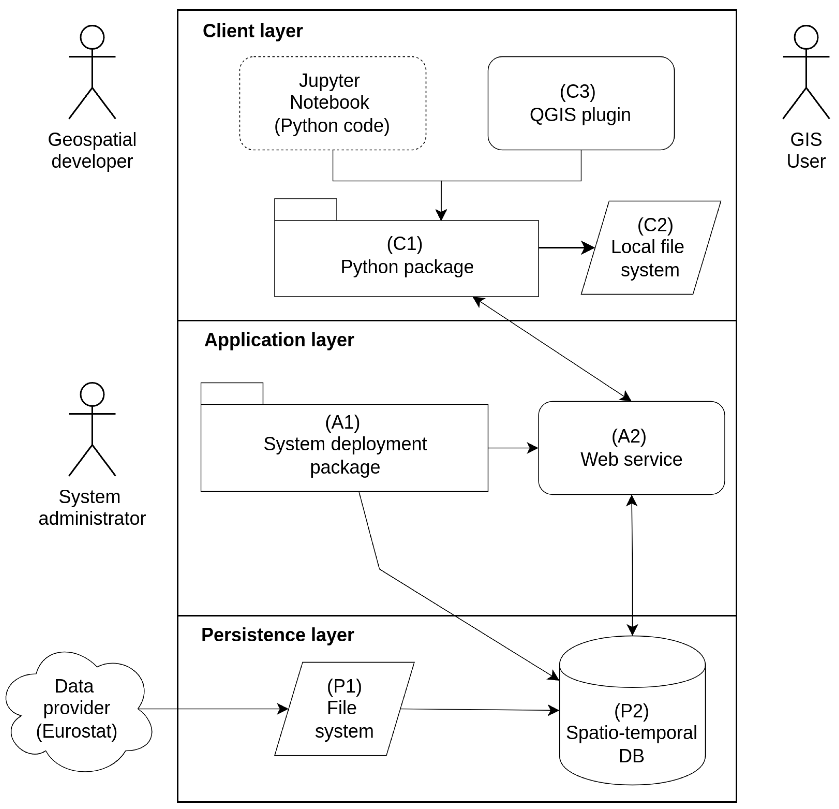
3.1. System High-Level Architecture

The system architecture follows a typical multi-layer client-server model customized to meet the objectives defined in Section 1. The system partitions the tasks between the server side with the LUCAS dataset and clients, and the users consuming the spatio-temporal subsets of the LUCAS data. Moreover, the design also follows the idea of Component-Based Software Engineering (CBSE) as described, for instance, by Vale et al. [47].
The system, as depicted in Figure 3, is decomposed into three main layers consisting of several components (Table 1) in each of the layers. The persistence layer provides a means to store the input, intermediate (separate years), and final harmonized space–time aggregated LUCAS data (O1). The main role of this layer is to preserve the data in non-volatile storage for further distribution. The main component of this layer is a database system (spatially enabled SQL database). The application layer provides the system deployment and harmonization (O2) procedures and the data distribution web service (O3). The distribution functionality is achieved by the OGC Web Feature Service. The client layer communicates through an internal interface with the data distribution service that provides harmonized LUCAS data to the end user. The client layer’s main functionality is provided by the Python software package. The main requirement is to create requests based on user-defined spatial, attribute, thematic, and temporal filters. The client layer provides two ways to retrieve and filter the subsets of the data (O4), through a command line interface (CLI) or through a graphical user interface (GUI). The client layer has an additional defined functionality to translate the LUCAS land cover nomenclature to other legends (O5) or aggregate the legend based on customer requirements.
The system is designed for three potential high-level users. The system administrator is able to deploy the system as it is designed or configure it for customized application use. The geospatial developer is able to access the harmonized LUCAS dataset through the Python API (e.g., using the Jupyter Notebook or directly by the Python code) in a fully automated processing pipeline. The GIS user is able to interactively explore and download the subsets of the LUCAS dataset via the desktop QGIS application (QGIS plugin).
The ST_LUCAS system is devised to allow full scalability. The vertical scalability may be achieved by deploying the system in a cloud environment. The horizontal scalability of the presented system may be achieved by adding multiple map server instances in the application layer.

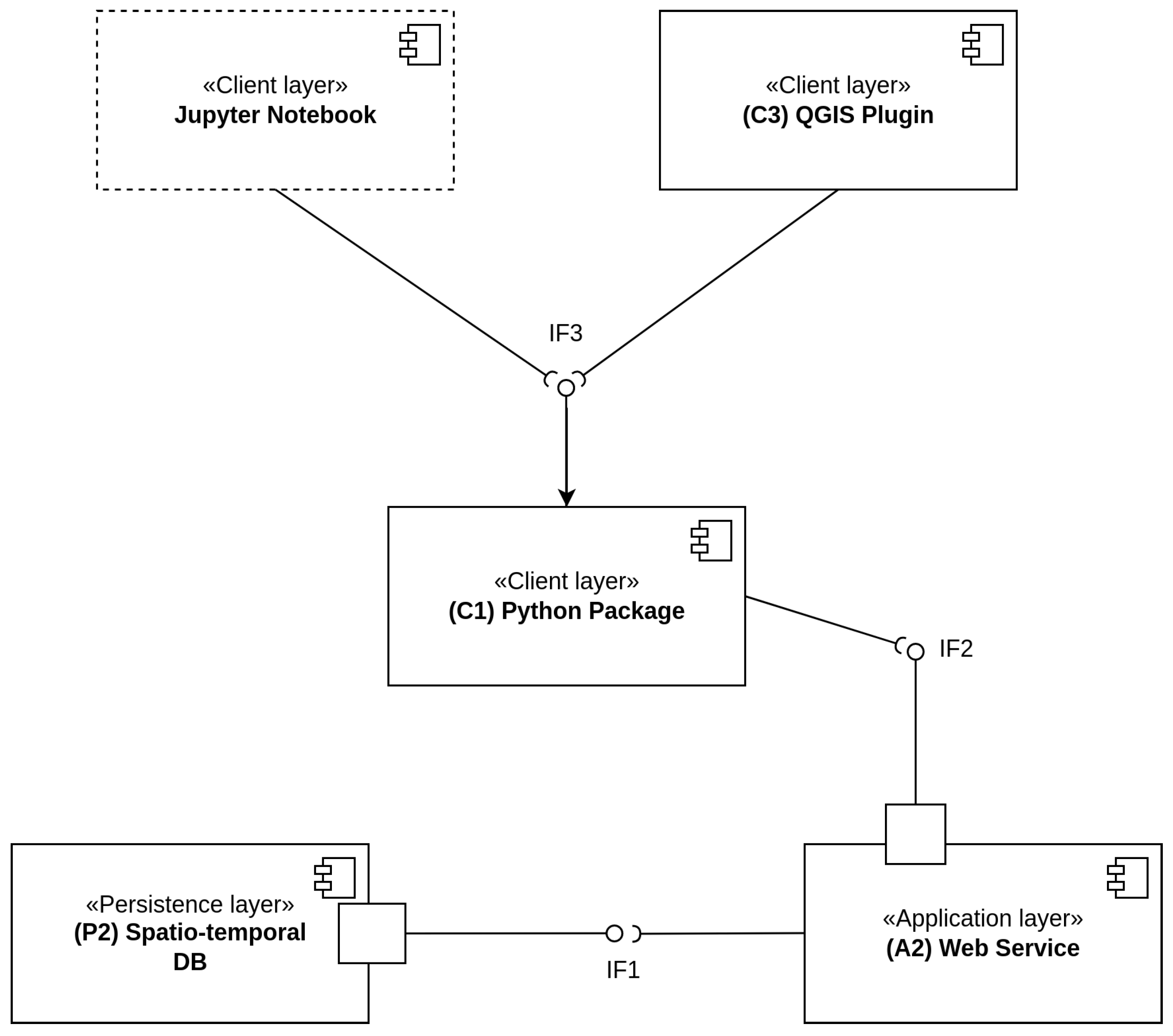
3.2. System Interfaces

The overall system is designed as encapsulated individual software components, which provide a set of related functions. The software components communicate with each other via interfaces [48]. There are two types of interfaces: internal interfaces and external interfaces. The internal and external interfaces are illustrated using the UML component diagram in Figure 4. The internal interface provides communication between the persistence layer and the application layer (IF1). It is an interface between the database system and the web service using the OGC WFS specification where harmonized LUCAS data flow. The other internal interface provides communication between the application layer (web service) and the client Python package (IF2), which is defined by the OGC WFS specification. The external interfaces are between the client application (CLI or GUI) and the client layer Python package (IF3). Here, the web service sends requests to the spatio-temporal database and the service provides harmonized LUCAS data to the end users’ client in the form of the Geography Markup Language (GML) features. A QGIS plugin/Jupyter Notebook (client layer) communicates with the ST_LUCAS system via the Python package API. This interface provides the access and functionalities to retrieve and filter harmonized spatio-temporal LUCAS data subsets from the application layer.

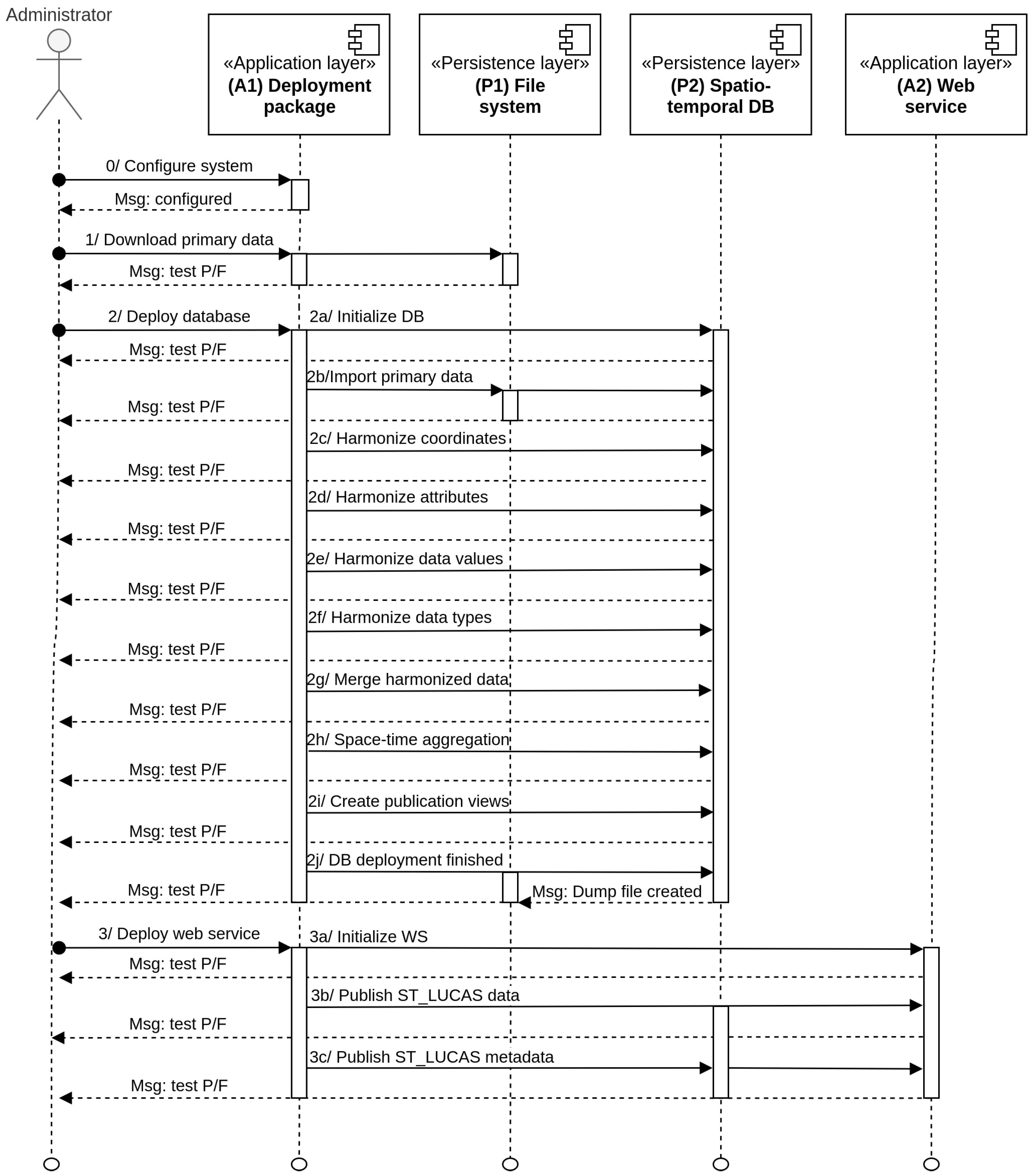
3.3. System Dynamic Architecture

The dynamic architecture was designed by means of UML sequential diagrams to plan the interactions of the above-designed system components over time. The dynamic architecture was divided into two phases: the system deployment phase and the user interaction process.
Figure 5 presents a UML sequential diagram in the deployment phase, which is the interaction between the main components of the application layer (deployment package and web service) and the persistence layer (file system and database system). The process starts with the configuration of the initial system, according to the administrator’s requirements. Next, the deployment package (A1) performs three major operations. Firstly, the LUCAS primary data distributed in the plain CSV format are automatically downloaded from the data provider specified in the system configuration. Secondly, after successfully downloading the primary CSV files to the server file system (P1), the database system (P2) is deployed. Deployment of the database system is split into ten sub-operations starting with a database initialization step and followed by importing the primary LUCAS data into the initialized database. The harmonization process includes the unification of spatial coordinates, attribute names, attribute data types, and data values. These operations are performed separately for each survey year. Subsequently, space–time aggregation of the harmonized LUCAS observations is applied. The deployment process is completed by creating a database dump file for the creation of the spatio-temporal database. Thirdly, the system web service (A2) component is deployed. Next, the harmonized LUCAS data in the database system may be published by the web service. Each of the sequential steps is followed by tests to evaluate the system performance.
Figure 6 presents a UML sequential diagram of the user interaction process. This process is the interaction between the main components of the client side (CLI/GUI clients—C3, Python package—C1) and the server side represented by the application layer web service (A2) providing the data from the persistence layer (database system—P2). In addition, the users’ local file system (C2) is introduced in Figure 3 to illustrate the dynamic interaction with the ST_LUCAS system.
The end user is able to interact with the system using a GUI designed for the open-source QGIS platform or through the Python API. The QGIS plugin (C3) is built on the top of the Python package (C1) allowing easy access to harmonized space–time LUCAS data. Alternatively, the Jupyter Notebook may be used for code-based data interaction in the Python programming language.
Initially, the server access has to be configured to access a web service (A2) through the Python package (C1) on the client side. As soon as the server (web service) provides information on the successful connection, the user is able to define the data requests. The user builds a request based on spatial, attribute, thematic, and temporal filters in order to obtain a subset of the harmonized LUCAS dataset. The request is sent to the server-side web service component (A2) by the Python package (C1). The response from the server comprises a subset of the harmonized LUCAS dataset that corresponds to the filters defined in the user’s request. The data retrieved from a web service (A2) are stored by the Python package (C1) on the local file system (C2).

3.4. System Validation

System validation is a constituent part of the system design. The validation is performed at two levels. At the design (documentation) level, which allows traceability between the model components in the architecture phase, and the software level to test each component and the interface of the designed system at the system deployment, execution, and external users’ access.
We defined unit tests for each software component according to the detailed architectural design of the system (Figure 3, Figure 4 and Figure 5). The ST_LUCAS system deployment process is controlled by the A1 software component. The process is formed by three major steps as shown in Figure 5: (1) download primary data (P1), (2) deploy database (P2), and (3) deploy web service (A2). Unit tests (1) validate the LUCAS primary data download process as specified in the configuration. The following set of unit tests (2) validates whether DB (P2) was initialized (2a), the primary data imported (2b), the LUCAS data harmonization process applied (2c–2h), the harmonized LUCAS data prepared for publication (2i), and the DB recovery file created (2j). The last set of unit tests (3) validates whether the web service (A2) is operational (3a) and the ST_LUCAS data (3b) and metadata (3c) are published. For the client layer, the unit tests cover the Python package (C1) and the local file system (C2) components. For the QGIS plugin (C3), manual verification is performed. An overview of the unit tests is depicted in Table 2. Each test is evaluated as successful if the test result is in compliance with the system configuration; otherwise, it is evaluated as failed.
The interaction between the software components is validated by integration tests. For each interface (Figure 4), a set of integration tests was designed (Table 3). Various combinations of spatial, temporal, attribute, and thematic filters are tested. A request based on a specified set of filters is built by the Python package (C1) and sent to the server. The web service (A2) returns a relevant subset of harmonized LUCAS data (IF2). The subset is compared with a recordset provided by a direct query to the database (P2) using SQL statements (IF1). The integration tests are evaluated with a pass result only if both interfaces (IF1 and IF2) return the same subset of the LUCAS data. The system administrator is notified about the integration test results regularly by email notifications. It ensures that system administrators will be informed about a potential system failure in real time, which is an important aspect of the operational deployment of the ST_LUCAS system. For the IF3 interface, manual verification was performed via the Jupyter Notebook.
The unit (Table 2) and integration (Table 3) tests are automated with the Python pytest package [49]. Verification is, therefore, performed during the software execution, which dynamically checks the software behavior. The unit test results are verified by the system administrator at the deployment phase. In the event that one of the unit tests fails, the deployment process is terminated, and the system is not deployed. The integration test results are verified repeatedly at the system execution phase. The result of each test operation is sorted in a log file, which is publicly available (Demonstration of the ST_LUCAS system, https://geoforall.fsv.cvut.cz/st_lucas, release 1.0 published by the authors on 9 June 2022) and may, therefore, be verified by the user.

4. System Implementation

The ST_LUCAS system implementation and deployment follow the design as described in Section 3. The system is completely based on open-source software components to ensure its reproducibility, transparency, and extensibility (Appendix A Table A1). Overall, the architecture splits the system into the client (frontend) and the server side (backend); hence, the implementation aspects are described separately.

4.1. Backend

The backend, the server side consisting of the persistence and application layers, is composed of software components that are responsible for the data storage, harmonization of LUCAS data, and data distribution. The components (represented in Figure 3) are implemented as a collection of services (see Section 4.3). Each service is managed in an isolated Docker container running on any operating system supported by the Docker virtualization technology [50]. There are two core backend software components: the database management system, operating a spatio-temporal DB (P2), and the map server, providing a web service (A2). The database management system is represented by an object-relational open-source PostgreSQL server [51]. This database system has a strong reputation for reliability, data integrity, and correctness. Moreover, it provides extension to geospatial data, the so-called PostGIS, which “spatially enables” the PostgreSQL database [52]. PostGIS also follows the OpenGIS “Simple Features Specification for SQL” by OGC. Here, we use the PostGIS version 3.1. The P2 and A2 components are deployed by the system deployment package (A1).
The database population process is controlled by a collection of scripts implemented in the Python 3 and Bash programming languages covering all steps as described in the dynamic system architecture (Figure 5). The harmonization process of the LUCAS data is procedural. It is decomposed as a series of computational steps carried out at the database level by scripts written in SQL. The configuration of the harmonization process is managed by a collection of CSV and JavaScript Object Notation (JSON) files. The robust but still easy-to-use configuration allows system administrators to affect the result of the harmonization process. In the same way, the system may be easily extended by new LUCAS observations planned to be published in 2022. The GDAL library [53] is used to import the primary LUCAS data from the file system (P1) to the PostGIS database tables (P2).
The web service (A2) is implemented as a map server, provided by the open-source GeoServer software version 2.19 [54]. The GeoServer is an OGC compliant implementation of a number of open standards such as the Web Map Service (WMS) and the Web Coverage Service (WCS). Additional formats and publication options are available as extensions, including the Web Processing Service (WPS) and the Web Map Tile Service (WMTS). It also conforms to the OGC WFS standard, which allows the sharing of the vector features to be used on the client side. Users are able to incorporate the LUCAS dataset into their processing pipelines and applications, freeing the data and permitting greater transparency. When the data becomes available from the deployment process, the GeoServer provides harmonized LUCAS data via a standardized WFS interface through Hypertext Transfer Protocol (HTTP).
The deployment package source code is available from the GitLab repository (https://gitlab.com/geoharmonizer_inea/st_lucas/st_lucas-system-deployment, release 1.0 published by the authors on 9 June 2022).

4.2. Frontend

The frontend, the client side, is composed of the Python package (C1) and the CLI client or GUI clients, as depicted in Figure 3. The Python package maintains the main functionality of the client side to be used by the end-user, either through the QGIS plugin (C3) without the necessity of any additionally programming/scripting, while the geospatial developer may use the Python API package directly to integrate harmonized LUCAS subsets into their own coded Earth observation pipelines.

4.2.1. Python Package

The frontend is developed based on the core component, the Python package (C1), which provides communication between the web server (A2) and the users’ clients through API. The package implemented in the Python 3 programming language consists of three modules: (1) request to create a request by specifying spatial, temporal, attribute, or thematic filters; (2) io to retrieve harmonized LUCAS data provided by the web service (A2) based on the submitted request, and to store the retrieved data in the user local file system (C2) in a specified data format; and (3) analyze to process the received harmonized LUCAS data—LUCAS land cover classes aggregation and nomenclature translation.
To use the Python API, the user creates a request by the LucasRequest Python class. In a single request, a combination of spatial, temporal, attribute, and thematic filters may be used. The spatial filter may be defined either by a bounding box, the NUTS0 country code, or by a user-defined polygon vector layer. Spatial coordinates must be specified in the ETRS89-extended/LAEA Europe coordinate reference system (EPSG 3035). The spatial filter is required by request; the other filters are optional. The temporal filter is specified by a list of survey years to be queried. The attribute filter is provided by an operator, an attribute name, and a list of values. The thematic filter defines the subset of harmonized LUCAS attributes to be retrieved. The example below (Listing 1) demonstrates the combination of all possible filters; the spatial filter is defined by a bounding box (request.bbox) covering the whole EU territory; the temporal filter (request.years) restricts the result to the 2015 and 2018 survey years; and the attribute filter (request.propertyname, request.operator, request.literal, and request.logical) selects only the LUCAS observations with land cover classes (LUCAS attribute LC1), C21 (Spruce dominated coniferous woodland), or C22 (Pine dominated coniferous woodland). The thematic filter (request.group) defines a subset of harmonized LUCAS attributes only to those which are relevant to the “Land Cover, Land Use” thematic group (LC_LU code in Appendix A Table A2).
Listing 1. Build a request.
from st_lucas import LucasRequest
from owslib.fes import PropertyIsEqualTo, Or

request = LucasRequest ()
request.bbox = (1510105, −2292253, 8582000, 5306000)
request.years = [2015, 2018]
request.propertyname = ‘LC1’
request.operator = PropertyIsEqualTo
request.literal = [‘C21’, ‘C22’]
request.logical = Or
request.group = ‘LC_LU’
The LUCAS subset retrieval according to the defined filters and data storage is managed by a LucasIO Python class. The LUCAS data are retrieved from the web service (A2) by the LucasIO.download() method based on the specified LucasRequest class instance. The number of retrieved LUCAS samples is returned by the LucasIO.count() method (Listing 2).
Listing 2. Download LUCAS subset based on the request.
from st_lucas import~LucasIO

lucasio = LucasIO ()
lucasio.download (request)
print (‘Number of LUCAS points:’, lucasio.count ())
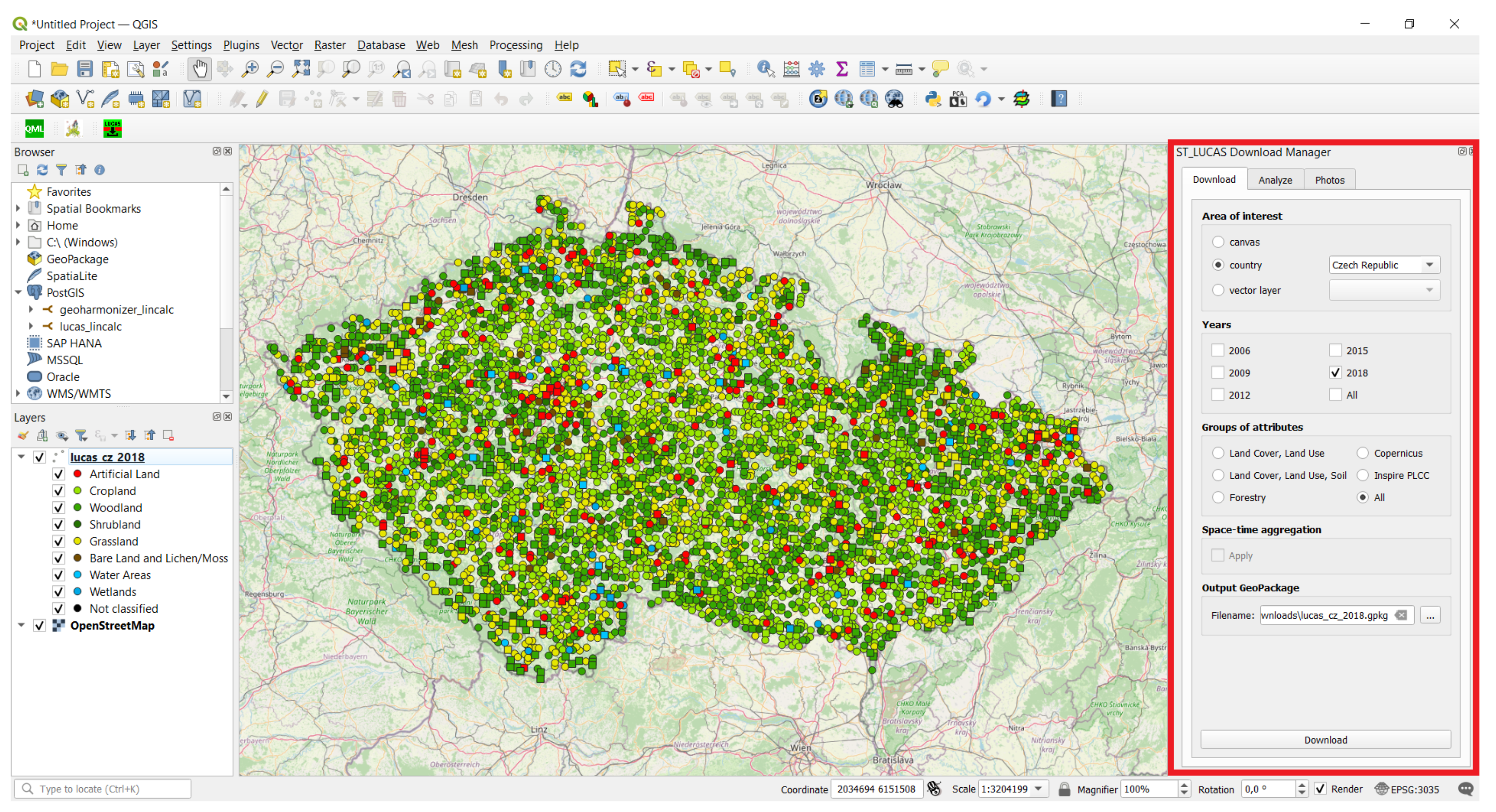
The downloaded LUCAS data may be stored on a local file system (C2) as an OGC GeoPackage file by the LucasIO.to_gpkg() method for further processing in GIS applications or converted by the LucasIO.to_geopandas() method into a GeoDataFrame object, which may be processed and analyzed in the Python code by the GeoPandas library [55].
The analyze Python module provides two analytical functionalities. The Python class LucasClassAggregate implements the LUCAS land cover classes aggregation. In addition to the aggregation of land cover classes, the module also offers the possibility of translating the LUCAS nomenclature into other nomenclatures using the LucasClassTranslate Python class. Complex Python API usage is demonstrated in several use cases and is discussed in Section 5.
The client Python API may be used directly by the Python code (CLI), running the Jupyter Notebook, or by the QGIS developed plugin (GUI). The Jupyter Notebook as a web-based interactive computing platform allows interactive data exploration [56] for geospatial developers. The Python package source code and the Jupyter Notebooks demonstrating the capabilities of the system are available in the GitLab repository (https://gitlab.com/geoharmonizer_inea/st_lucas/st_lucas-python-package, release 1.0 published by the authors on 9 June 2022).

4.2.2. QGIS Plugin

Another option for harmonized space–time LUCAS dataset exploration is to use the ST_LUCAS QGIS plugin. The plugin is a GUI integrated into the open-source QGIS platform. The user interface (Figure 7) is split into three tabs: (1) Download; (2) Analyze; and (3) Photos. The added value of using GIS is to interactively select the spatial, attribute, temporal, and thematic filters from the GUI (Download tab). In particular, it enables selection of an area of interest (spatial filter) by the extent of the map canvas, specification of a country from a list of EU countries or use of a user-defined vector polygon data layer. The plugin interface allows a list of selected years (temporal filter) and a group of attributes (thematic filter) to also be specified. There are five thematic groups in total to choose from, where each group contains specific thematic attributes in addition to the basic attributes. The following groups are available: Land Cover, Land Use; Land Cover, Land Use, Soil; Forestry; Copernicus; and Inspire PLCC (Appendix A Table A2). The user is also able to download LUCAS points with all available attributes.
The Analyze tab integrates functionality for performing a user-defined class aggregation using a JSON file and a nomenclature translation using a CSV file. An example of usage is included in the plugin documentation available online on the ST_LUCAS website (https://geoforall.fsv.cvut.cz/st_lucas/qgis_plugin/, release 1.0 published by the authors on 9 June 2022).
Users are also able to browse photos (a facing photo and four landscape photos in the cardinal compass directions) of a selected LUCAS point in the Photo tab (Figure 8) as provided by the GISCO service [57].
The subset of harmonized space–time LUCAS data retrieved from the server is stored in the OGC GeoPackage format with a predefined style for further usage. The style of LUCAS points is defined to distinguish the land cover classes at the first level of the LUCAS nomenclature as shown in Figure 7. In addition, points with a circular symbol indicate that photos are available for display. Points with a square symbol indicate the opposite.
The QGIS plugin source code is available in the GitLab repository (https://gitlab.com/geoharmonizer_inea/st_lucas/st_lucas-qgis-plugin, release 1.0 published by the authors on 9 June 2022).

4.3. ST_LUCAS System Deployment

In order to enhance the portability of the developed ST_LUCAS system, the Docker virtualization technology [50] was employed. All the backend components are deployed through virtualization. There are four deployed services managed by the Docker-compose tool, each running in an isolated Docker container: (1) db: responsible for the spatio-temporal database (P2) deployment including harmonized space–time LUCAS data; (2) gs: responsible for running a map server providing the OGC WFS service (A2); (3) gsp: responsible for publishing harmonized space–time LUCAS data as a WFS service. The publication process is performed when the database deployment is successfully completed. At this point, the system metadata and documentation are also populated. The service is terminated when the publishing process is successfully completed; and (4) gst: performs repetitive integration tests (Table 3) controlling whether the system is operational. Logs are publicly available; and the system administrator is notified by email.
The ST_LUCAS system deployment controls components in the persistence and application layers as shown in Figure 3. The spatio-temporal DB (P2) is managed by a Docker container (db), which mounts the server file system (P1) as a volume. As the system deployment package (A1) manages all the deployment steps, it is available to all Docker containers (db, gs, gsp, and gst) through the mounted volume.
The complete deployment of the ST_LUCAS system is performed by a single command: docker-compose up.
The demonstration ST_LUCAS system installation, available at https://geoforall.fsv.cvut.cz/st_lucas (release 1.0 published by the authors on 9 June 2022), is deployed on GNU/Debian operating system version 11.

5. Discussion

The developed ST_LUCAS system has multiple uses. System managers may take the system and install it (Docker containers) in their institutes as it is (objective O1). Geospatial developers may utilize (e.g., configure) the current system and let it run for their own purposes (O2). Geospatial users may access the harmonized spatio-temporal LUCAS dataset, and its subsets, using either the machine-to-machine Python API or the interactive QGIS plugin (O4). The data are provided by a standardized interface defined by OGC WFS (O3). The system offers developers and geospatial users full and configurable automation of the harmonization process for past and future LUCAS survey updates, spatio-temporal and thematic subsetting of the data based on user-defined filters, land cover legend translation to a defined nomenclature, and legend aggregation (O5).
Next, we demonstrate and discuss the use of the ST_LUCAS system via two use cases (Section 5.1 and Section 5.2), in addition to the use of the system described by Witjes et al. [29] for the European scale land cover mapping between 2000 and 2019.

5.1. LUCAS Data for Land Cover Change Analysis

In the first use case, we demonstrate how to retrieve a vector of changing land cover from the ST_LUCAS system. Assuming the geospatial user wants to calibrate the classification change model or validate the existing land cover change product, we need to retrieve a subset of data with repeated visits on the same geographical points. The task may be simply set up by selecting LUCAS points where repeated visits are higher than one. As mentioned in Section 1, a total of 319,150 sample points are visited at least twice, and 35,204 samples are visited five times.
Below, a Python snippet code (Listing 3) demonstrates how to retrieve LUCAS points with repeated visits for land cover change analysis using the SURVEY_COUNT attribute for AOI (areas of interest) in the Czech Republic. There were 11,084 points retrieved with the initial spatial and temporal filter, while by adding the condition SURVEY_COUNT > 1 we received a subset of 6175 points.
Listing 3. Build a request for land cover change analysis.
from st_lucas import LucasRequest
from owslib.fes import~PropertyIsGreaterThan

request = LucasRequest ()

request.countries = [‘CZ’]
request.st_aggregated = True
request.group = ‘LC_LU’

request.propertyname = ‘SURVEY_COUNT’
request.operator = PropertyIsGreaterThan
request.literal = 1
In Figure 9, we illustrate an example of the land cover change vector (LC1 codes: B16, B15, B55, E10, and E20) for the case of five in situ repeated visits (2006, 2009, 2012, 2015, and 2018), together with orthophotos in the background. It clearly shows the changing landscape documented by the orthophotos and the changing LC codes in the LUCAS database.

5.2. LUCAS Data for Land Product Validation

In the next use case, we demonstrate the use of LUCAS data for land product validation. In this case, validation of the national-level Land Parcel Identification System (LPIS) of the Czech Republic for 2018, which is an open dataset [58]. We simplified the validation into two agriculture classes, cropland (class 1) and grassland (class 2), which represent the majority of the agricultural land in LPIS. Initially, we retrieved the subset of LUCAS data with the respective spatial and temporal filters in the validation process, similarly to the code snippet in Listing 1. Next, we used the LucasClassAggregate Python class from the developed Python package to simplify the nomenclature to the above-defined legend (Listing 4). The method’s argument is a Python dictionary defining the class mappings for the aggregation process.
Listing 4. Perform land cover class aggregation.
from st_lucas import~LucasClassAggregate

lc1_to_agri = {
“1”: [“B11”, “B12”, “B13”, “B14”, “B15”, “B16”, “B17”, “B18”,
      “B19”, “B21”, “B22”, “B23”, “B31”, “B32”, “B33”, “B34”,
      “B35”, “B36”, “B37”, “B41”, “B42”, “B43”, “B44”, “B45“
      “B51”, “B52”, “B53”, “B54”, “B55”, “B71”, “B72”, “B73”,
      “B74”, “B75”, “B76”, “B77”, “B81”, “B82”, “B83”, “B84”],
“2”: [“E10”, “E20”, “E30”]
}

lucasaggr = LucasClassAggregate(lucasio.data, mappings=lc1_to_agri)
lucasaggr.apply ()
The retrieved vector layer with the aggregated nomenclature was overlaid with the LPIS product and validation indicators were calculated (Table 4). It is possible to conclude that the LPIS product has a high thematic accuracy, with an overall F1-score of 96%, compared to the LUCAS in situ survey of 2018.

6. Conclusions

This article presents a developed ST_LUCAS geospatial data system. A versatile open-source framework for the LUCAS dataset harmonization, distribution by the OGC compliant interface, Python client API and QGIS plugin to retrieve subsets of data, and methods to manage nomenclature translation, class aggregation, and thematic information. The source code, documentation, and installation instructions are publicly available on GitLab (https://gitlab.com/geoharmonizer_inea/st_lucas, release 1.0 published by the authors on 9 June 2022). The ST_LUCAS deployment package and the Python client package are published under the MIT license, the QGIS plugin under GNU GPL v3.
The system is designed in a multi-layer client-server model allowing integration to end-to-end workflows. Integration of the system into full end-to-end workflows is facilitated by the Python API. The transferability of the system to different server end-points is facilitated by OS-level virtualization using Docker containers. This allows a diverse audience of geospatial developers and scientists to use the capabilities of the ST_LUCAS system in their own environments. Moreover, the system may be configured based on specific user requirements. The system is prepared for the new LUCAS survey of 2022 as soon as it is publicly available.
We discuss the use of the ST_LUCAS system via two use cases (Section 5). The workflow management capabilities have been already tested to prepare a harmonized spatio-temporal LUCAS dataset for the European scale land cover mapping between 2000 and 2019 [29]. The experience gained from this large-scale use case proved the necessity of auxiliary methods for the land cover nomenclature translation and aggregation, which is not a common feature in purely distribution systems.
Overall, we believe the ST_LUCAS system provides better accessibility and usability of the European LUCAS dataset through a standardized OGC interface. The specific enhancement is in the space–time aggregation of the data that emphasizes the use of a highly valuable in situ survey database for change analysis as a priority of all land monitoring projects. In addition, the ST_LUCAS system is fully integrated into the QGIS desktop platform, allowing interactive exploration of the LUCAS data and direct GIS analysis. As a continuation of the ST_LUCAS development, we plan to run extended demonstration use cases. In particular, we intend to explore the value of repeated in situ visits for land cover change detection. To fulfill this task, we shall develop translation tables from the LUCAS land cover legend to various nomenclatures. Furthermore, we shall explore the spatial representativeness of the sampled points in order to use the data for validation and land cover calibration activities in varying spatial resolutions.
The ST_LUCAS system was implemented based on current knowledge of the primary data acquired in 2018 and the previous surveys performed since 2006. The system may require future updates according to changes in the LUCAS dataset from subsequent surveys.

Author Contributions

Conceptualization, Martin Landa and Lukáš Brodský; methodology, Martin Landa, Lukáš Brodský and Lena Halounová; software, Martin Landa, Tomáš Bouček and Ondřej Pešek; validation, Martin Landa and Tomáš Bouček; formal analysis, Lukáš Brodský; investigation, Lukáš Brodský; resources, Lukáš Brodský; data curation, Tomáš Bouček; writing—original draft preparation, Lukáš Brodský, Martin Landa and Tomáš Bouček; writing—review and editing, Lena Halounová and Ondřej Pešek; visualization, Martin Landa, Lukáš Brodský and Tomáš Bouček; supervision, Lena Halounová; project administration, Martin Landa; and funding acquisition, Martin Landa. All authors have read and agreed to the published version of the manuscript.

Funding

This research was funded by the Grant Agreement Connecting Europe Facility (CEF) Telecom project grant number 2018-EU-IA-0095 Geo-harmonizer project (2019–2022).

Institutional Review Board Statement

Not applicable.

Informed Consent Statement

Not applicable.

Data Availability Statement

The LUCAS primary data are available from EUROSTAT free of charge to all users (https://ec.europa.eu/eurostat/en/web/lucas/data/primary-data, accessed on 26 April 2022).

Acknowledgments

Administrative and technical support by the Faculty of Civil Engineering, Czech Technical University in Prague. The authors would like to thank reviewers for taking the time and effort necessary to review the manuscript. The authors sincerely appreciate all valuable comments and suggestions, which helped to improve the quality of the manuscript.

Conflicts of Interest

The authors declare no conflict of interest.

Abbreviations

The following abbreviations are used in this manuscript:
APIApplication Programming Interface
CBSEComponent-Based Software Engineering
CLICommand Line Interface
CSVComma Separated Values (file format)
EPSGEPSG Geodetic Parameter Dataset
EUEuropean Union
EUNISEuropean Nature Information System
GISGeographic Information System
GUIGraphical User Interface
HTTPHypertext Transfer Protocol
INSPIREInfrastructure for Spatial Information in Europe
JSONJavaScript Object Notation
LCLand Cover
LUCAS Land Use and Coverage Area frame Survey
NUTSNomenclature of Territorial Units for Statistics
OGCOpen Geospatial Consortium
PLCCPure Land Cover Components
SDISpatial data Infrastructure
SQLStructured Query Language
UMLUnified Modeling Language
WCSWeb Coverage Service
WFSWeb Feature Service
WMSWeb Map Service
WMTSWeb Map Tile Service
WPSWeb Processing Service

Appendix A

Table A1. Open-source software used by the ST_LUCAS system. Component IDs reflect the system architecture as presented in Figure 3.
Component IDSoftwareLicense
P2PostgreSQLPostgreSQL licence
P2PostGISGNU GPL
A1Docker CEN/A (free of charge)
A1Docker ComposeApache License 2.0
A1psycopg2 *GNU LGPL v3
A1gdal *MIT
A1pytest *MIT
A1owslib *BSD 3
A1geoserver-rest *MIT
A1requests *Apache 2.0
A2GeoServerGNU GPL
C1json/os/csv/logging/tempfile/pathlib/shutil *PSF 2.2/BSD 0
C1gdal *MIT
C1owslib *BSD 3
C1requests *Apache 2.0
C3QGISGNU GPL
* Python package.
Table A2. List of ST_LUCAS attributes.
AttributeGroupDescriptionUnitsOrigin
POINT_IDDEFAULTUnique point identifier Primary
NUTS0DEFAULTNUTS Lvl 0 Primary
NUTS1DEFAULTNUTS Lvl 1 Primary
NUTS2DEFAULTNUTS Lvl 2 Primary
NUTS3DEFAULTNUTS Lvl 3 Primary
SURVEY_DATEDEFAULTDate of observationyyyy-mm-ddHarmonized
CAR_LATITUDEDEFAULTGPS Car parking latitude°Primary
CAR_LONGITUDEDEFAULTGPS Car parking longitude°Primary
CAR_EWDEFAULTGPS Car parking East/West1: East, 2: West, —1: Not RelevantPrimary
GPS_PROJDEFAULTGPS Projection1: WGS84, 2: GPS Problem, —1: Not RelevantHarmonized
GPS_PRECDEFAULTGPS PrecisionmPrimary
GPS_LATDEFAULTGPS Observation latitude°Harmonized
GPS_EW GPS Observation East/West1: East, 2: West, —1: Not RelevantHarmonized
GPS_LONGDEFAULTGPS Observation longitude°Harmonized
GPS_ALTITUDEDEFAULTGPS altitudemPrimary
GEOG_GPSDEFAULTPostGIS geography (EPSG 4326) generated from GPS_LAT, GPS_LONG New
GEOM_GPSDEFAULTPostGIS geometry (EPSG 3035) generated from GPS_LAT, GPS_LONG New
GEOM_REPR_AREADEFAULTPostGIS geometry (EPSG 3035) of representative area New
TH_LATDEFAULTTheoretical Latitude°Primary
TH_EW Theoretical East/West1: East, 2: West, —1: Not RelevantHarmonized
TH_LONGDEFAULTTheoretical Longitude°Primary
GEOG_THDEFAULTPostGIS geography (EPSG 4326) generated from TH_LAT, TH_LONG New
GEOM_THRDEFAULTPostGIS geography (EPSG 3035) generated from TH_LAT, TH_LONG snapped to LUCAS grid New
GEOMDEFAULTPostGIS geometry (EPSG 3035) generated from measured GPS location (GEOM_GPS) if no GPS problem detected otherwise theoretical location (GEOM_THR) New
DIST_THR_GRIDDEFAULTDistance computed from GEOG_THR and LUCAS gridmNew
OBS_DISTDEFAULTGPS Distance to theoretical pointmHarmonized
OBS_DIRECTDEFAULTDirection of observation in case of linear feature1: on the point, 2: Look to the North, 3: Look to the East, —1: Not RelevantPrimary
OBS_TYPEDEFAULTObservation type1: In Situ < 100 m, 2: In Situ > 100 m, 3: In Situ PI, 4: In Situ PI not possible, 5: Out of national territory, 6: Out of EU28, 7: In Office PI, —1: Not RelevantHarmonized
OBS_RADIUSDEFAULTRadius of observation circle1: 1.5 m, 2: 20 m, —1: Not RelevantPrimary
LC1LAND COVER (LC_LU, LC_LU_SO)Land Cover 1 Primary
LC1_HLAND COVER (LC_LU, LC_LU_SO)Harmonized Land Cover 1 to 2018 nomenclature—1: Not RelevantNew
LC1_H_L3_MISSINGLAND COVER (LC_LU, LC_LU_SO)Harmonized Land Cover 1 on lvl 1 or lvl 2 if lvl 3 is missing New
LC1_H_L3_MISSING _LEVELLAND COVER (LC_LU, LC_LU_SO)Level of available land cover 1 value if lvl 3 is missing1: Level 1, 2: Level 2New
LC1_SPECLAND COVER (LC_LU, LC_LU_SO)Land Cover 1 Species—1: Not RelevantHarmonized
LC1_PERCLAND COVER (LC_LU, LC_LU_SO)Percentage of coverage of Land Cover 1%, —1: Not RelevantHarmonized
LC1_PERC_CLSLAND COVER (LC_LU, LC_LU_SO)Percentage of coverage of Land Cover 1 by codes1: 10%, 2: 25%, 3: 50%, 4: 75%, 5: 100%, —1: Not RelevantNew
LC2LAND COVER (LC_LU, LC_LU_SO)Land Cover 2 Primary
LC2_HLAND COVER (LC_LU, LC_LU_SO)Harmonized Land Cover 2 to 2018 nomenclature—1: Not RelevantNew
LC2_H_L3_MISSINGLAND COVER (LC_LU, LC_LU_SO)Harmonized Land Cover 2 on lvl 1 or lvl 2 if lvl 3 is missing New
LC2_H_L3_MISSING_LEVELLAND COVER (LC_LU, LC_LU_SO)Level of available land cover 2 value if lvl 3 is missing1: Level 1, 2: Level 2New
LC2_SPECLAND COVER (LC_LU, LC_LU_SO)Land Cover 2 Species—1: Not RelevantHarmonized
LC2_PERCLAND COVER (LC_LU, LC_LU_SO)Percentage of coverage of Land Cover 2%, —1: Not RelevantHarmonized
LC2_PERC_CLSLAND COVER (LC_LU, LC_LU_SO)Percentage of coverage of Land Cover 2 by codes1: 10%, 2: 25%, 3: 50%, 4: 75%, 5: 100%, —1: Not RelevantNew
LU1LAND USE (LC_LU, LC_LU_SO)Land Use 1 Primary
LU1_HLAND USE (LC_LU, LC_LU_SO)Harmonized Land Use 1 to 2018 nomenclature—1: Not RelevantNew
LU1_TYPELAND USE (LC_LU, LC_LU_SO)Land Use 1 species—1: Not RelevantPrimary
LU1_PERCLAND USE (LC_LU, LC_LU_SO)Percentage of coverage of Land Use 1%, —1: Not RelevantHarmonized
LU1_PERC_CLSLAND USE (LC_LU, LC_LU_SO)Percentage of coverage of Land Use 1 by codes1: 5%, 2: 10%, 3: 25%, 4: 50%, 5: 75%, 6: 90%, 7: 100%, —1: Not RelevantNew
LU2LAND USE (LC_LU, LC_LU_SO)Land Use 2 Primary
LU2_HLAND USE (LC_LU, LC_LU_SO)Harmonized Land Use 2 to 2018 nomenclature—1: Not RelevantNew
LU2_TYPELAND USE (LC_LU, LC_LU_SO)Land Use 2 species—1: Not RelevantPrimary
LU2_PERCLAND USE (LC_LU, LC_LU_SO)Percentage of coverage of Land Use 2%, —1: Not RelevantHarmonized
LU2_PERC_CLSLAND USE (LC_LU, LC_LU_SO)Percentage of coverage of Land Use 2 by codes1: 5%, 2: 10%, 3: 25%, 4: 50%, 5: 75%, 6: 90%, 7: 100%, —1: Not RelevantNew
PARCEL_AREA_HALAND USE (LC_LU, LC_LU_SO)Parcel Area - area of the parcel which the point belongs to1: <0.1 ha, 2: 0.1–0.5 ha, 3: 0.5–1 ha, 4: 1–10 ha, 5: >10 ha, —1: Not RelevantHarmonized
TREE_HEIGHT_SURVEYTREE PROPERTIES (FO)Height of trees at survey time1: <5 m, 2: >5 m, —1: Not RelevantPrimary
TREE_HEIGHT_MATURITYTREE PROPERTIES (FO)Height of trees at maturity1: <5 m, 2: >5 m, —1: Not RelevantPrimary
FEATURE_WIDTHLAND COVER (LC_LU, LC_LU_SO)Feature width1: <20 m, 2: >20 m, —1: Not RelevantPrimary
LM_PLOUGH_SLOPELAND MANAGEMENT (LC_LU, LC_LU_SO)Slope of ploughed field1: Flat, 2: Gently sloping, 3: Steeply sloping, 4: Undulating, —1: Not RelevantPrimary
LM_PLOUGH_DIRECTLAND MANAGEMENT (LC_LU, LC_LU_SO)Plough direction1: Across the slope, 2: Down the slope, 3: Not Applicable, —1: Not RelevantPrimary
LM_STONE_WALLSLAND MANAGEMENT (LC_LU, LC_LU_SO)Presence of stone walls1: No, 2: Stone wall not mantained, 3: Stone wall well mantained, —1: Not RelevantPrimary
LM_GRASS_ MARGINSLAND MANAGEMENT (LC_LU, LC_LU_SO)Presence of grass margins1: No, 2: Grass margin < 1 m, 3: Grass margin > 1 m, —1: Not RelevantPrimary
CPRN_CANDOCOPERNICUS LAND COVER (CO)Copernicus taken1: Yes, 2: No, —1: Not RelevantPrimary
CPRN_LCCOPERNICUS LAND COVER (CO)Copernicus Land Cover Primary
CPRN_LC1NCOPERNICUS LAND COVER (CO)Extension of LC North Primary
CPRNC_LC1ECOPERNICUS LAND COVER (CO)Extension of LC East Primary
CPRNC_LC1SCOPERNICUS LAND COVER (CO)Extension of LC South Primary
CPRNC_LC1WCOPERNICUS LAND COVER (CO)Extension of LC West Primary
CPRN_LC1N_BRDTHCOPERNICUS LAND COVER (CO)Percentage of breadth North%, —1: Not RelevantPrimary
CPRN_LC1E_BRDTHCOPERNICUS LAND COVER (CO)Percentage of breadth East%, —1: Not RelevantPrimary
CPRN_LC1S_BRDTHCOPERNICUS LAND COVER (CO)Percentage of breadth South%, —1: Not RelevantPrimary
CPRN_LC1W_BRDTHCOPERNICUS LAND COVER (CO)Percentage of breadth West%, —1: Not RelevantPrimary
CPRN_LC1N_NEXTCOPERNICUS LAND COVER (CO)Next copernicus Land Cover North Primary
CPRN_LC1E_NEXTCOPERNICUS LAND COVER (CO)Next copernicus Land Cover East Primary
CPRN_LC1S_NEXTCOPERNICUS LAND COVER (CO)Next copernicus Land Cover South Primary
CPRN_LC1W_NEXTCOPERNICUS LAND COVER (CO)Next copernicus Land Cover West Primary
CPRN_URBANURBAN (CO)Point in Urban area1: Yes, 2: No, —1: Not RelevantPrimary
CPRN_IMPERVIOUS _PERCIMPERVIOUS (CO)Percentage of imperviousness%, —1: Not RelevantPrimary
INSPIRE_PLCC1INSPIRE PLCC (IN)Percentage of Coniferous forest trees%, —1: Not RelevantPrimary
INSPIRE_PLCC2INSPIRE PLCC (IN)Percentage of Broadleaved forest trees%, —1: Not RelevantPrimary
INSPIRE_PLCC3INSPIRE PLCC (IN)Percentage of Shrubs%, —1: Not RelevantPrimary
INSPIRE_PLCC4INSPIRE PLCC (IN)Percentage of herbaceous plants%, —1: Not RelevantPrimary
INSPIRE_PLCC5INSPIRE PLCC (IN)Percentage of Lichens and mosses%, —1: Not RelevantPrimary
INSPIRE_PLCC6INSPIRE PLCC (IN)Percentage of consolidated bare land%, —1: Not RelevantPrimary
INSPIRE_PLCC7INSPIRE PLCC (IN)Percentage of unconsolidated bare land%, —1: Not RelevantPrimary
INSPIRE_PLCC8INSPIRE PLCC (IN)Percentage of other land%, —1: Not RelevantPrimary
EUNIS_COMPLEXEUNIS (LC_LU)EUNIS Complex6: X06, 9: X09, 10: Other, 11: Unknown, —1: Not RelevantPrimary
GRASSLAND _SAMPLEGRASS (LC_LU)Sample Grassland module0: FALSE, 1: TRUEPrimary
GRASS_CANDOGRASS (LC_LU)Grassland taken1: Yes, 2: No, —1: Not RelevantPrimary
GRAZINGLAND USE (LC_LU, LC_LU_SO)Signs of grazing1: Visible sighns of grazing, 2: No sighn of grazing, —1: Not RelevantHarmonized
WMLAND USE (LC_LU, LC_LU_SO)Presence of Water Management1: Irrigation, 2: Potential irrigation, 3: Drainage, 4: Irrigation and drainage, 5: No visible Water management, —1: Not RelevantPrimary
WM_SOURCELAND USE (LC_LU, LC_LU_SO)Source of irrigation1: Well, 2: Pond/Lake/Reservoir, 3: Stream/Canal/Ditch, 4: Lagoon/Wastewater, 5: Other/Not identifiable, —1: Not RelevantHarmonized
WM_TYPELAND USE (LC_LU, LC_LU_SO)Type of irrigation1: Gravity, 2: Pressure sprinkler irrigation, 3: Pressure micro-irrigation, 4: Gravity/Pressure, 5: Other/Not identifiable, —1: Not RelevantHarmonized
WM_DELIVERYLAND USE (LC_LU, LC_LU_SO)Delivery System1: Canal, 2: Ditch, 3: Pipeline, 4: Other/Not identifiable, —1: Not RelevantHarmonized
SOIL_TAKENSOIL (LC_LU_SO)Soil taken1: Yes, 2: Not possible, 3: No, already taken, 4: No sample required, —1: Not RelevantHarmonized
EROSION_CANDOSOIL (LC_LU_SO)Erosion taken1: Yes, 2: No, —1: Not RelevantPrimary
BIO_SAMPLESOIL (LC_LU_SO)Sample bio soil module0: FALSE, 1: TRUEPrimary
SOIL_BIO_TAKENSOIL (LC_LU_SO)Bio soil taken0: FALSE, 1: TRUE, —1: Not RelevantPrimary
BULK0_10_SAMPLESOIL (LC_LU_SO)Sample bulk 0–10 module0: FALSE, 1: TRUEPrimary
SOIL_BLK_0_10 _TAKENSOIL (LC_LU_SO)Bulk 0–10 taken1: Yes, 2: No, —1: Not RelevantPrimary
BULK10_20_SAMPLESOIL (LC_LU_SO)Sample bulk 10–20 module0: FALSE, 1: TRUEPrimary
SOIL_BLK_10_20 _TAKENSOIL (LC_LU_SO)Bulk 10–20 taken1: Yes, 2: No, —1: Not RelevantPrimary
BULK20_30_SAMPLESOIL (LC_LU_SO)Sample bulk 20–30 module0: FALSE, 1: TRUEPrimary
SOIL_BLK_20_30 _TAKENSOIL (LC_LU_SO)Bulk 20–30 taken1: Yes, 2: No, —1: Not RelevantPrimary
STANDARD_SAMPLESOIL (LC_LU_SO)Sample standard soil module0: FALSE, 1: TRUEPrimary
SOIL_STD_TAKENSOIL (LC_LU_SO)Standard soil taken1: Yes, 2: No, —1: Not RelevantPrimary
ORGANIC_SAMPLESOIL (LC_LU_SO)Sample organic soil module0: FALSE, 1: TRUEPrimary
SOIL_ORG_DEPTH _CANDOSOIL (LC_LU_SO)Organic soil taken1: Yes, 2: No, —1: Not RelevantPrimary
OFFICE_PIDEFAULTSample photo interpreted in office0: FALSE, 1: TRUEHarmonized
PI_EXTENSIONDEFAULTPoint on extened part of survey (photo-interpreted)0: FALSE, 1: TRUEPrimary
LNDMNG_PLOUGHLAND USE (LC_LU, LC_LU_SO)Signs of ploughing1: Yes, 2: No, —1: Not RelevantPrimary
SPECIAL_STATUSLAND USE (LC_LU, LC_LU_SO)Special status1: Protected, 2: Hunting, 3: Protected and hunting, 4: No special status, —1: Not RelevantPrimary
LC_LU_SPECIAL _REMARKLAND COVER (LC_LU, LC_LU_SO)Special remarks in LC/LU1: Harvested field, 2: Tilled/sowed, 3: Clear cut, 4: Burnt area, 5: Fire break, 6: Nursey, 7: Dump site, 8: Temporary dry, 9: Temporary flooded, 10: No remark, —1: Not RelevantHarmonized
SOIL_STONES _PERCSOIL (LC_LU_SO)Percentage of Stones on the surface%, —1: Not RelevantHarmonized
SOIL_STONES _PERC_CLSSOIL (LC_LU_SO)Percentage of Stones on the surface by codes1: 5%, 2: 20%, 3: 40%, 4: 75%, —1: Not RelevantNew
PHOTO_POINTLAND COVER (LC_LU, LC_LU_SO)Photo point taken1: Taken, 2: Not Taken, —1: Not RelevantPrimary
PHOTO_NORTHLAND COVER (LC_LU, LC_LU_SO)Photo north taken1: Taken, 2: Not Taken, —1: Not RelevantPrimary
PHOTO_EASTLAND COVER (LC_LU, LC_LU_SO)Photo east taken1: Taken, 2: Not Taken, —1: Not RelevantPrimary
PHOTO_SOUTHLAND COVER (LC_LU, LC_LU_SO)Photo south taken1: Taken, 2: Not Taken, —1: Not RelevantPrimary
PHOTO_WESTLAND COVER (LC_LU, LC_LU_SO)Photo west taken1: Taken, 2: Not Taken, —1: Not RelevantPrimary
CROP_RESIDUESLAND COVER (LC_LU, LC_LU_SO)Presence of crop residues1: Yes, 2: No, —1: Not RelevantHarmonized
TRANSECTLAND COVER (LC_LU, LC_LU_SO)Transect LC sequence Primary
EX_ANTEDEFAULTVisited in the field0: FALSE, 1: TRUEPrimary
SURVEY_YEARDEFAULTSurvey year New
SURVEY_COUNTSPACE-TIMENumber of visits New
SURVEY_DISTSPACE-TIMEDistance computed from representative location (GEOM) and measured GPS location (GEOM_GPS)mNew
SURVEY_MAXDISTSPACE-TIMEMaximum distance computed from representative location (GEOM) and measured GPS location (GEOM_GPS)mNew

References

  1. Akitsu, T.K.; Nasahara, K.N. In-Situ observations on a moderate resolution scale for validation of the Global Change Observation Mission-Climate ecological products: The uncertainty quantification in ecological reference data. Int. J. Appl. Earth Obs. Geoinf. 2022, 107, 102639. [Google Scholar] [CrossRef]
  2. Lee, J.G.; Kang, M. Geospatial Big Data: Challenges and Opportunities. Big Data Res. 2015, 2, 74–81. [Google Scholar] [CrossRef]
  3. Ishwarappa; Anuradha, J. A Brief Introduction on Big Data 5Vs Characteristics and Hadoop Technology. Procedia Comput. Sci. 2015, 48, 319–324. [Google Scholar] [CrossRef] [Green Version]
  4. Koubarakis, M.; Stamoulis, G.; Bilidas, D.; Ioannidis, T.; Pantazi, D.A.; Vlassov, V.; Payberah, A.H.; Wang, T.; Sheikholeslami, S.; Hagos, D.H.; et al. Artificial Intelligence and big data technologies for Copernicus data: The EXTREMEEARTH project. In Proceedings of the 2021 Conference on Big Data from Space, Virtual Event, 18–20 May 2021; pp. 9–12. [Google Scholar] [CrossRef]
  5. Overview—Land Cover/Use Statistics. Available online: https://ec.europa.eu/eurostat/web/lucas (accessed on 11 April 2022).
  6. Bettio, M.; Delincé, J.; Bruyas, P.; Croi, W.; Eiden, G. Area frame surveys: Aim, Principals and Operational Surveys. In Building Agri-Environmental Indicators, Focussing on the European Area Frame Survey LUCAS; Eurostat: Luxembourg, 2002; pp. 12–27. [Google Scholar] [CrossRef]
  7. Fritz, S.; McCallum, I.; Schill, C.; Perger, C.; Grillmayer, R.; Achard, F.; Kraxner, F.; Obersteiner, M. Geo-Wiki.Org: The Use of Crowdsourcing to Improve Global Land Cover. Remote Sens. 2009, 1, 345–354. [Google Scholar] [CrossRef] [Green Version]
  8. Defourny, P.; Mayaux, P.; Herold, M.; Bontemps, S. Global land-cover map validation experiences: Toward the characterization of quantitative uncertainty. In Remote Sensing of Land Use and Land Cover; Giri, C.P., Ed.; CRC Press: Boca Raton, FL, USA, 2016; pp. 207–223. [Google Scholar] [CrossRef]
  9. Close, O.; Benjamin, B.; Petit, S.; Fripiat, X.; Hallot, E. Use of Sentinel-2 and LUCAS Database for the Inventory of Land Use, Land Use Change, and Forestry in Wallonia, Belgium. Land 2018, 7, 154. [Google Scholar] [CrossRef] [Green Version]
  10. Weigand, M.; Staab, J.; Wurm, M.; Taubenböck, H. Spatial and semantic effects of LUCAS samples on fully automated land use/land cover classification in high-resolution Sentinel-2 data. Int. J. Appl. Earth Obs. Geoinf. 2020, 88, 102065. [Google Scholar] [CrossRef]
  11. Pflugmacher, D.; Rabe, A.; Peters, M.; Hostert, P. Mapping pan-European land cover using Landsat spectral-temporal metrics and the European LUCAS survey. Remote Sens. Environ. 2019, 221, 583–595. [Google Scholar] [CrossRef]
  12. Gao, Y.; Liu, L.; Zhang, X.; Chen, X.; Mi, J.; Xie, S. Consistency Analysis and Accuracy Assessment of Three Global 30-m Land-Cover Products over the European Union using the LUCAS Dataset. Remote Sens. 2020, 12, 3479. [Google Scholar] [CrossRef]
  13. d’Andrimont, R.; Yordanov, M.; Martinez-Sanchez, L.; Eiselt, B.; Palmieri, A.; Dominici, P.; Gallego, J.; Reuter, H.I.; Joebges, C.; Lemoine, G.; et al. Harmonised LUCAS In-Situ land cover and use database for field surveys from 2006 to 2018 in the European Union. Sci. Data 2020, 7, 352. [Google Scholar] [CrossRef]
  14. Borrelli, P.; Poesen, J.; Vanmaercke, M.; Ballabio, C.; Hervás, J.; Maerker, M.; Scarpa, S.; Panagos, P. Monitoring gully erosion in the European Union: A novel approach based on the Land Use/Cover Area frame survey (LUCAS). Int. Soil Water Conserv. Res. 2022, 10, 17–28. [Google Scholar] [CrossRef]
  15. Jeppesen, J.H.; Ebeid, E.; Jacobsen, R.H.; Toftegaard, T.S. Open geospatial infrastructure for data management and analytics in interdisciplinary research. Comput. Electron. Agric. 2018, 145, 130–141. [Google Scholar] [CrossRef]
  16. Wiemann, S.; Brauner, J.; Karrasch, P.; Henzen, D.; Bernard, L. Design and prototype of an interoperable online air quality information system. Environ. Model. Softw. 2016, 79, 354–366. [Google Scholar] [CrossRef]
  17. Li, W.; Wang, S.; Bhatia, V. PolarHub: A large-scale web crawling engine for OGC service discovery in cyberinfrastructure. Comput. Environ. Urban Syst. 2016, 59, 195–207. [Google Scholar] [CrossRef] [Green Version]
  18. Klug, H.; Kmoch, A. A SMART groundwater portal: An OGC web services orchestration framework for hydrology to improve data access and visualisation in New Zealand. Comput. Geosci. 2014, 69, 78–86. [Google Scholar] [CrossRef]
  19. Best, B.D.; Halpin, P.N.; Fujioka, E.; Read, A.J.; Qian, S.S.; Hazen, L.J.; Schick, R.S. Geospatial web services within a scientific workflow: Predicting marine mammal habitats in a dynamic environment. Ecol. Inform. 2007, 2, 210–223. [Google Scholar] [CrossRef]
  20. Rosatti, G.; Zorzi, N.; Zugliani, D.; Piffer, S.; Rizzi, A. A Web Service ecosystem for high-quality, cost-effective debris-flow hazard assessment. Environ. Model. Softw. 2018, 100, 33–47. [Google Scholar] [CrossRef]
  21. Rautenbach, V.; Coetzee, S.; Iwaniak, A. Orchestrating OGC web services to produce thematic maps in a spatial information infrastructure. Comput. Environ. Urban Syst. 2013, 37, 107–120. [Google Scholar] [CrossRef] [Green Version]
  22. Web Feature Service|OGC. Available online: https://www.ogc.org/standards/wfs (accessed on 11 April 2022).
  23. OGC API—Features. Available online: https://ogcapi.ogc.org/features/ (accessed on 11 April 2022).
  24. Giuliani, G.; Ray, N.; Lehmann, A. Grid-enabled Spatial Data Infrastructure for environmental sciences: Challenges and opportunities. Future Gener. Comput. Syst. 2011, 27, 292–303. [Google Scholar] [CrossRef] [Green Version]
  25. Blauth, D.A.; Ducati, J.R. A Web-based system for vineyards management, relating inventory data, vectors and images. Comput. Electron. Agric. 2010, 71, 182–188. [Google Scholar] [CrossRef]
  26. Zioti, F.; Ferreira, K.R.; Queiroz, G.R.; Neves, A.K.; Carlos, F.M.; Souza, F.C.; Santos, L.A.; Simoes, R.E.O. A platform for land use and land cover data integration and trajectory analysis. Int. J. Appl. Earth Obs. Geoinf. 2022, 106, 102655. [Google Scholar] [CrossRef]
  27. Data—Land Cover/Use Statistics. Available online: https://ec.europa.eu/eurostat/web/lucas/data (accessed on 11 April 2022).
  28. Eurostat Regional Yearbook 2021. Available online: https://ec.europa.eu/statistical-atlas/viewer/ (accessed on 11 April 2022).
  29. Witjes, M.; Parente, L.; van Diemen, C.; Hengl, T.; Landa, M.; Brodsky, L.; Halounova, L.; Krizan, J.; Antonic, L.; Ilie, C.; et al. A spatiotemporal ensemble machine learning framework for generating land use/land cover time-series maps for Europe (2000–2019) based on LUCAS, CORINE and GLAD Landsat. PeerJ-Life Environ. 2022; accepted. [Google Scholar] [CrossRef]
  30. LUCAS Primary Data 2006. Available online: https://ec.europa.eu/eurostat/en/web/lucas/data/primary-data/2006 (accessed on 8 April 2022).
  31. LUCAS Primary Data 2009. Available online: https://ec.europa.eu/eurostat/en/web/lucas/data/primary-data/2009 (accessed on 8 April 2022).
  32. LUCAS Primary Data 2012. Available online: https://ec.europa.eu/eurostat/en/web/lucas/data/primary-data/2012 (accessed on 8 April 2022).
  33. LUCAS Primary Data 2015. Available online: https://ec.europa.eu/eurostat/en/web/lucas/data/primary-data/2015 (accessed on 8 April 2022).
  34. LUCAS Primary Data 2018. Available online: https://ec.europa.eu/eurostat/en/web/lucas/data/primary-data/2018 (accessed on 8 April 2022).
  35. LUCAS Grid—Land Cover/Use Statistics. Available online: https://ec.europa.eu/eurostat/web/lucas/data/lucas-grid (accessed on 8 April 2022).
  36. LUCAS 2009. Technical Reference Document C3 Classification (Land Cover & Land Use). Available online: https://ec.europa.eu/eurostat/documents/205002/208938/LUCAS2009_C3-Classification_20121004.pdf (accessed on 27 May 2020).
  37. LUCAS 2012. Technical Reference Document C3 Classification (Land Cover & Land Use). Available online: https://ec.europa.eu/eurostat/documents/205002/208012/LUCAS_2012_C3-Classification_20131004_0.pdf (accessed on 27 May 2020).
  38. LUCAS 2015. Technical Reference Document C3 Classification (Land Cover & Land Use). Available online: https://ec.europa.eu/eurostat/documents/205002/6786255/LUCAS2015_C3-Classification_20160729.pdf (accessed on 27 May 2020).
  39. LUCAS 2018. Technical Reference Document C3 Classification (Land Cover & Land Use). Available online: https://ec.europa.eu/eurostat/documents/205002/8072634/LUCAS2018-C3-Classification.pdf (accessed on 27 May 2020).
  40. Contents of the 2006 Lucas Primary Data. Available online: https://ec.europa.eu/eurostat/documents/205002/209869/Contents_LUCAS_2006_primary_data.xls (accessed on 27 May 2020).
  41. LUCAS Survey 2009 Technical Reference Document c-1: Instructions for Surveyors. Available online: https://ec.europa.eu/eurostat/documents/205002/208938/LUCAS+2009+Instructions (accessed on 27 May 2020).
  42. LUCAS Survey 2012 Technical Reference Document c-1: Instructions for Surveyors. Available online: https://ec.europa.eu/eurostat/documents/205002/208012/LUCAS2012_C1-InstructionsRevised_20130110b.pdf (accessed on 27 May 2020).
  43. LUCAS Survey 2015 Web CSV Record Descriptor. Available online: https://ec.europa.eu/eurostat/documents/205002/6786255/WebCsv_RecordDescriptor20161006.pdf (accessed on 27 May 2020).
  44. LUCAS Survey 2018 Web CSV Record Descriptor. Available online: https://ec.europa.eu/eurostat/documents/205002/8072634/LUCAS2018-RecordDescriptor-190611.pdf (accessed on 27 May 2020).
  45. PostGIS Documentation—ST_GeometricMedian. Available online: https://postgis.net/docs/ST_GeometricMedian.html (accessed on 11 April 2022).
  46. Weiszfeld, E.; Plastria, F. On the point for which the sum of the distances to n given points is minimum. Ann. Oper. Res. 2009, 167, 7–41. [Google Scholar] [CrossRef]
  47. Vale, T.; Crnkovic, I.; de Almeida, E.S.; da Mota Silveira Neto, P.A.; Cavalcanti, Y.C.; de Lemos Meira, S.R. Twenty-eight years of component-based software engineering. J. Syst. Softw. 2016, 111, 128–148. [Google Scholar] [CrossRef]
  48. Nierstrasz, O.; Meijler, T.D. Research Directions in Software Composition. ACM Comput. Surv. 1995, 27, 262–264. [Google Scholar] [CrossRef]
  49. Pytest: Helps You Write Better Programs—Pytest Documentation. Available online: https://docs.pytest.org/en/7.1.x/ (accessed on 13 April 2022).
  50. Merkel, D. Docker: Lightweight Linux Containers for Consistent Development and Deployment. Linux J. 2014, 2014, 2. Available online: https://dl.acm.org/doi/10.5555/2600239.2600241 (accessed on 13 April 2022).
  51. PostgreSQL: The World’s Most Advanced Open-Source Database. Available online: https://www.postgresql.org/ (accessed on 13 April 2022).
  52. PostGIS Documentation. Available online: https://postgis.net/ (accessed on 13 April 2022).
  53. GDAL Documentation. Available online: https://gdal.org/ (accessed on 13 April 2022).
  54. GeoServer Documentation. Available online: https://geoserver.org/ (accessed on 13 April 2022).
  55. GeoPandas Documentation. Available online: https://geopandas.org/en/stable/ (accessed on 13 April 2022).
  56. Perkel, J.M. BY Jupyter, it all makes sense. Nature 2018, 563, 145–146. [Google Scholar] [CrossRef] [Green Version]
  57. Reference Data—GISCO. Available online: https://gisco-services.ec.europa.eu/lucas/photos/ (accessed on 11 April 2022).
  58. Land Parcel Identification System–LPIS. Available online: https://eagri.cz/public/app/lpisext/lpis/verejny2/plpis/ (accessed on 1 February 2022).
Figure 1. Distance between GPS measured and theoretical points (OBS_DIST attribute). A total of 35,509 points with a distance of more than 1000 m are not shown in this figure.
Ijgi 11 00361 g001
Figure 2. Space–time aggregation of observed LUCAS GPS locations (circle symbol) using the geometrical median (diamond symbol). The theoretical location snapped to a LUCAS 2 × 2 km 2 grid is represented by a rectangle symbol. The distances between the GPS and median locations are shown by arrowed dashed lines.
Ijgi 11 00361 g002
Figure 3. Static high-level architecture of the ST_LUCAS system. The Jupyter Notebook (dotted line) is not intended to be a software component. The Jupyter Notebook is used in this work to present the functionality of the Python package (C1) and to provide manual verification.
Ijgi 11 00361 g003
Figure 4. ST_LUCAS system software components with defined interfaces.
Ijgi 11 00361 g004
Figure 5. ST_LUCAS dynamic architecture (system deployment).
Ijgi 11 00361 g005
Figure 6. ST_LUCAS dynamic architecture of the system user interaction.
Ijgi 11 00361 g006
Figure 7. ST_LUCAS QGIS plugin (highlighted by a red box) retrieving harmonized LUCAS data for the Czech Republic territory (background basemap: OpenStreetMap—public WMS view service).
Ijgi 11 00361 g007
Figure 8. Showing LUCAS photos from the GISCO service by the ST_LUCAS QGIS plugin.
Ijgi 11 00361 g008
Figure 9. Example of changing land cover over time for POINT_ID = 46642928 as recorded in the LUCAS dataset (background orthophotos: Czech State Administration of Land Surveying and Cadastre—public WMS view service).
Ijgi 11 00361 g009
Table 1. Overview of the ST_LUCAS system components.
IDNameLayerRoleObjective
P1File systemPersistenceStore primary dataO1
P2DatabasePersistenceStore and provide harmonized dataO1
A1Deployment packageApplicationDeploy the system including data harmonizationO2
A2Web serviceApplicationProvide access to harmonized data through a web serviceO3
C1Python packageClientAPI interface to a web service and a set of analytical functionsO4, O5
C2Local file systemClientStore locally harmonized LUCAS dataO4, O5
C3QGIS pluginClientProvide GUI interface via GIS to a web service and a set of selected analytical functionsO4, O5
Table 2. Overview of unit tests. Test IDs reflect the system dynamic architecture as presented in Figure 5.
Component IDTest IDsDescription
A1, P11_001Primary data are downloaded according to the system configuration.
A1, P22a_001DB is initialized according to the system configuration.
2b_001-003Primary data are imported according to the system configuration.
2c_001-002Coordinates are harmonized according to the system configuration.
2d_001Attributes are harmonized according to the system configuration.
2e_001-002Data values are harmonized according to the system configuration.
2f_001Data types are harmonized according to the system configuration.
2g_001-004Harmonized data are merged according to the system configuration.
2h_001-003Data are space–time aggregated according to the system configuration.
2i_001-004Publication views are created according to the system configuration.
2j_001DB recovery file is created according to the system configuration.
A1, A23a_001-003Test case consists of checking OGC WFS operations: GetCapabilities, DescribeFeatureType and GetFeature.
3b_001-003ST_LUCAS dataset available via WFS.
3c_001-003The test cases consist of checking that ST_LUCAS metadata are published according
to the deployed database.
C1, C2001-007Test cases consist of checking LucasRequest and LucasIO classes methods to build a request, download a LUCAS subset, store retrieved data on the local file system, and access associated photos.
Table 3. Overview of integration tests. Interface IDs reflect the system architecture as presented in Figure 4.
Interface IDTest IDsDescription
IF1, IF2001–004Test cases consist of checking WFS responses retrieved by the Python package (IF2) covering various combinations of spatial, attribute, thematic, and temporal filters. The responses are compared with the subsets retrieved from spatio-temporal DB via SQL statements (IF1). Test cases pass only if there is no difference between the WFS responses and the subsets retrieved from DB.
Table 4. LPIS validation indicators.
ClassCodeSupportF1-ScorePrecisionRecall
Cropland1194198.197.199.1
Grassland269094.196.192.1
Overall 263196.197.195.1
Publisher’s Note: MDPI stays neutral with regard to jurisdictional claims in published maps and institutional affiliations.

