
Efficient Calculation of Distance Transform on Discrete Global Grid Systems


Department of Computer Science, University of Calgary, Calgary, AB T2N 1N4, Canada
*
Author to whom correspondence should be addressed.
ISPRS Int. J. Geo-Inf. 2022, 11(6), 322; https://doi.org/10.3390/ijgi11060322
Submission received: 25 March 2022
/
Revised: 17 May 2022
/
Accepted: 21 May 2022
/
Published: 25 May 2022
(This article belongs to the Special Issue Next-Generation Digital Earth Systems: From Geometric Modelling to Visualization)
Abstract
:Geospatial data analysis often requires the computing of a distance transform for a given vector feature. For instance, in wildfire management, it is helpful to find the distance of all points in an area from the wildfire’s boundary. Computing a distance transform on traditional Geographic Information Systems (GIS) is usually adopted from image processing methods, albeit prone to distortion resulting from flat maps. Discrete Global Grid Systems (DGGS) are relatively new low-distortion globe-based GIS that discretize the Earth into highly regular cells using multiresolution grids. In this paper, we introduce an efficient distance transform algorithm for DGGS. Our novel algorithm heavily exploits the hierarchy of a DGGS and its mathematical properties and applies to many different DGGSs. We evaluate our method by comparing its speed and distortion with the distance transform methods used in traditional GIS and general 3D meshes. We demonstrate that our method is efficient and has minimal distortion.
1. Introduction
We are gathering an immense amount of data about the Earth which has a great potential to help us understand and predict geospatial phenomena through analysis and simulation. For this, determining the distance of all points of a given region to a geospatial feature (e.g., boundary of a wildfire) is needed. Distance transform (DT) is a mapping that specifies the distance of all points in a domain to a specified feature and is a fundamental and frequent operation to perform analyses and simulation of geographic data. It has been used for various geospatial analyses including watershed delineation [1], urban planning [1], pipeline route design [2,3], and mountain railway alignment [4].
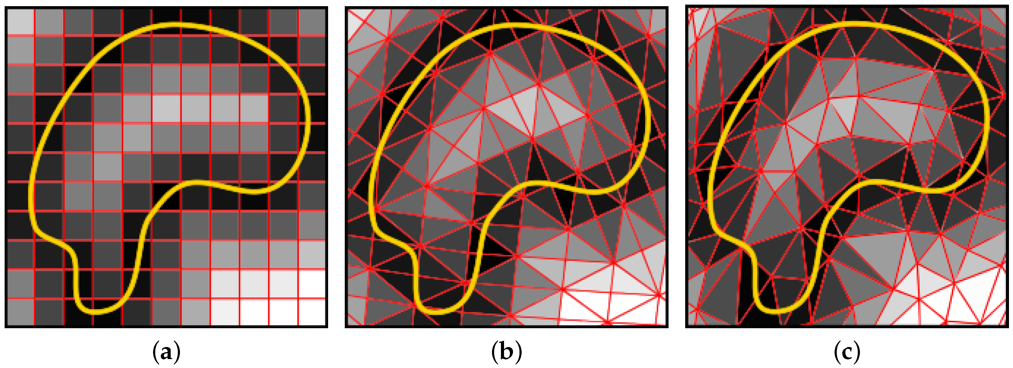
Traditional Geographic Information Systems (GIS) are usually based on flat maps, and they have adopted distance transform methods from image processing techniques [1,5]. Figure 1a shows distance transform applied to a feature inside of an image (i.e., regular 2D grid). Mapping the curved earth into a flat domain introduces distortion, consequently, any distance transform in image space may contain distortion. When a large area is projected, this projection distortion is greater. Therefore, the traditional GIS approach for distance transform is not directly applicable to large scale applications such as pipeline route design [2]. Aside from the distortion at large scales, similar to many other operations for the Earth, DT can be better presented and interpreted on the globe rather than 2D maps.
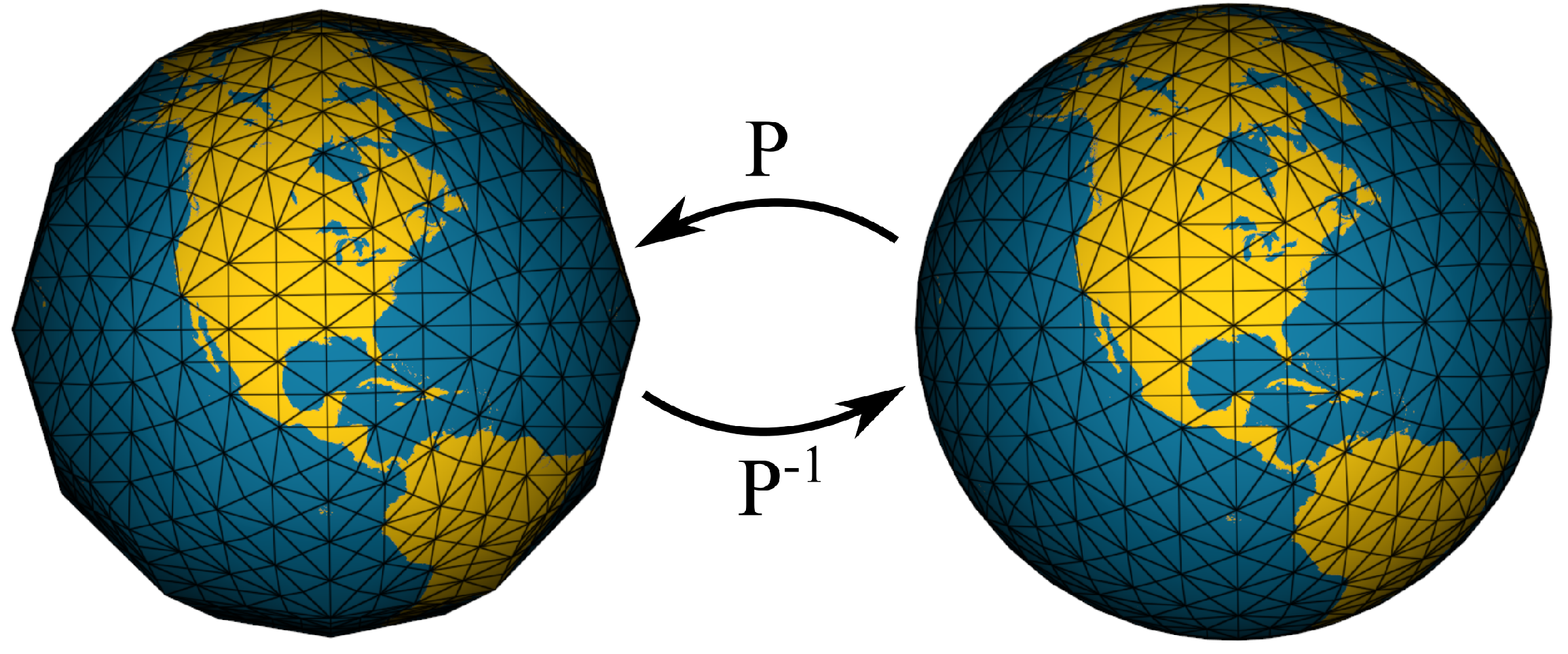
A new GIS approach, Discrete Global Grid Systems (DGGS), is a globe-based representation of the Earth that reduces distortion by approximating the Earth with a polyhedron [6,7,8]. A DGGS discretizes the Earth into mostly regular cells using multiresolution grid systems. The regularity and multiresolution properties of DGGS are the outcome of the iterative application of a refinement scheme to the initial polyhedron faces [6]. Due to the spherical nature of the globe, it is not possible to find a fully regular discretization for it. Hence, every DGGS grid is only semi-regular which makes it more challenging than a fully regular grid. However, there is a possibility of exploiting this semi-regularity to develop a more efficient algorithm in comparison with irregular grids (see Figure 1b,c). In the context of general 3D meshes, DT algorithms are developed based on geodesic distance calculations [9,10]. These general mesh algorithms can be applied to the DGGS grid but are slower, especially with larger grids. For the DGGS grid, we can use specific properties of DGGS to develop a more efficient algorithm. The traditional distance transform algorithms work on either perfectly regular grids (i.e., images) or general meshes. These methods are not fit for the semi-regular mesh of a DGGS and do not exploit the hierarchy of the underlying multiresolution grid. Thus, a novel approach is needed. To address this need, in this paper, we introduce a new, efficient distance transform algorithm for DGGS.
In DGGS, we define distance transform as the distance of a set of cells to one or a set of features. We use the properties of a DGGS, especially the hierarchy and the geometry of the DGGS, to design an efficient distance transform algorithm. This algorithm does not make any assumptions about the shape of the DGGS cells, the type of the refinement, and the underlying projection, which is an advantage and makes this algorithm applicable to many DGGSs.
Our algorithm is based on coarse to fine hierarchical traversal of the DGGS. We start with a coarse resolution and calculate the distance of each coarse cell to the feature. This step is efficient because there is a small number of cells in this resolution. Next, based on calculated distances on the current coarse resolution, we reduce the search space for the cells in higher resolutions and store all the relevant edges of the feature in a data structure. We then iteratively refine the grid to a higher resolution and make use of the pre-calculated search space to find the distance of child cells to the feature. We show that the distance of the child cells is guaranteed to fall within the proximity of parent cells.
We prove a mathematical theorem which allows us to design an efficient algorithm. We also analyse and report the performance of our algorithm for different input parameters. This algorithm is compared to image-based and general mesh-based methods. This comparison shows that our algorithm reduces distance distortions compared to methods that work on image space and mesh space. In terms of efficiency, this algorithm is faster compared to general mesh-based algorithms for higher resolutions. In summary, the main contribution of this paper is the development of a novel and efficient algorithm for computing a distance transform for a DGGS.
2. Background
In this section, we discuss background information for this paper. We explain related works and papers to state our work among others. This section starts with the definition of DT and its applications. Then, the necessary information about DGGS to understand this work is explained. Next, we discuss different algorithms and methods used to compute the DT on various domains as well as the advantages and disadvantages of each method.
2.1. Distance Transform Definition and Applications
In 1966, Rosenfeld et al. introduced DT as a sequential operation in digital picture processing with applications in shape skeletonization [11]. In the very basic form on Image Space, DT is a transformation from a binary image in which black pixels are object(s) or feature and white pixels are background, to a gray-scale image. In this gray-scale image, the gray level shows the distance of a background pixel to the feature. Figure 2 shows the distance transform applied to a binary image. By looking at Figure 2b, it is obvious that the skeleton of the shape can be extracted by following the bright pixels of the image.
After that, the idea of DT has been applied to many different areas and has applications in medical image processing [12,13], shape analysis [14,15,16], computer graphics [17], shortest path computation [18], image segmentation [19], and Convolutional Neural Networks [20], to name a few. In addition, different distance metrics such as Manhattan distance [11], Chessboard distance [21,22], and Chamfer distance [23] have also been used to find distance transform. However, Euclidean distance is still required for many of these applications [24].
Besides the various mentioned applications of DT, de Smith [1] showed that DT is useful for many geospatial applications too. For example, DT may be used for computation of multilevel buffer zones for watershed delineation and slope lines [1]. DT is also useful to construct voronoi regions which is useful for urban planing such as building hospitals and schools in a city or to manage a rescue team in an area [1]. Furthermore, DT has been used for large-scale construction planning such as pipeline route design [2,3], and mountain railway alignment [4]. Smart agriculture is another example which makes use of DT. When sampling soil from a field, DT can be used to ensure sample points are far enough away from the undesirable areas such as the boundary of the field or known areas of contamination [25].
2.2. Discrete Global Grid Systems
DGGS is a novel approach to GIS which approximates the Earth with a polyhedron to make a global, universal representation of the Earth with less distortion compared to flat maps [6]. DGGS is a discretized, hierarchical, and cell-based representation of the Earth that provides an efficient neighbourhood access and parent-child traversal [6,7]. Every DGGS is made of the following main elements.
2.2.1. Elements of a DGGS
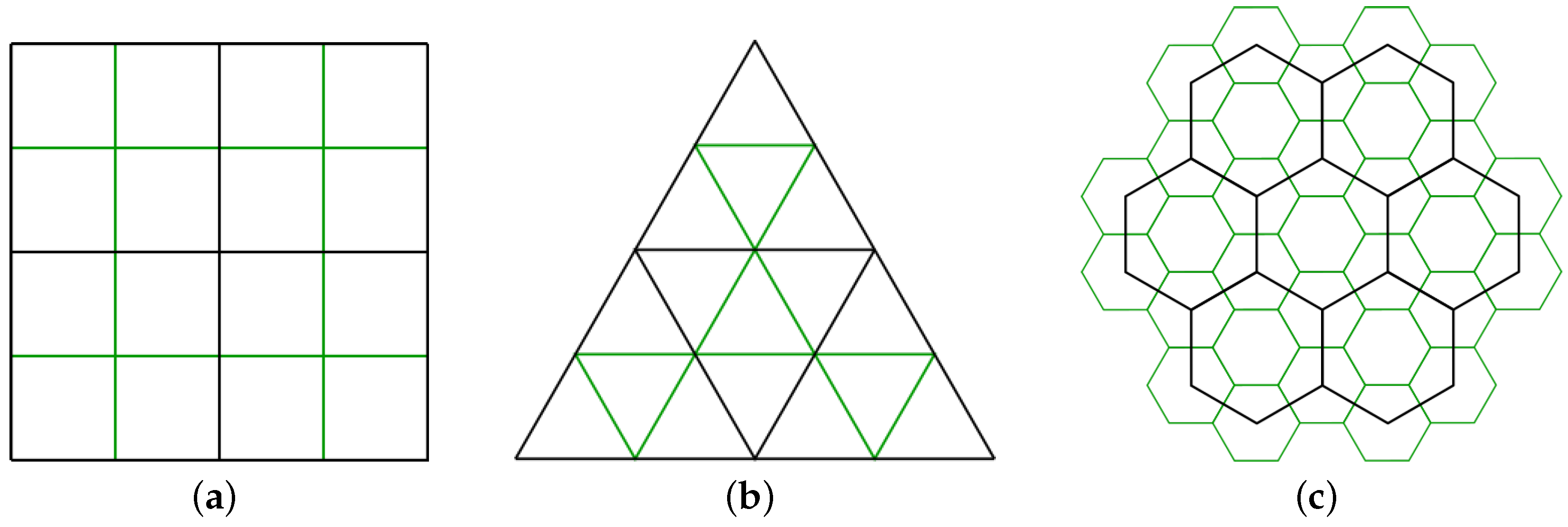
- Refinement Scheme: Cells resulted from the faces of the initial polyhedron are usually considered as the first resolution of the DGGS (i.e., zero level of refinement). A refinement scheme is applied to the faces of the polyhedron to make higher resolutions and a set of finer cells. This refinement can be congruent or non-congruent [6,7]. Figure 4 shows examples of refinements. The resolution at which the data is being presented is the target resolution of the DGGS. Figure 5 shows the Disdyakis Triacontahedron DGGS at different refinement levels [26]. At resolution 1, the average area of the Disdyakis Triacontahedron DGGS cells is around 4,250,546.6 km2. As this DGGS uses a 1 to 4 refinement, each consecutive resolution reduces the area by a factor of . This results in an average area of 15.4 m 2 at resolution 20.
- Cell Indexing: To assign and retrieve data to and from the cells, we need to assign some indices to the cells. Each index uniquely identifies one cell of the DGGS and a database can rely on these indices instead of coordinates to store the data.
2.2.2. Distance in DGGS
The real distance between two points on the Earth depends on the topology of the Earth between those two points. However, this distance is difficult to compute, which is why an approximation of the Earth is often used to measure distances between points. In this work, the distance between two points is calculated on a spherical domain via great-circle arc (i.e., geodesic) calculations. We use a DGGS to project the points to the spherical domain. Then, we use the following formula to calculate the distance between the two points of p and q (see Figure 7) with r representing the radius of the Earth.
2.3. Computing Distance Transform
While a DGGS has benefits over a traditional GIS, the problem of distance transform on DGGS is not investigated in the literature. In this section, we see how distance transform is computed in image space and mesh space. Image space is the perfectly regular end of the spectrum where distance transform algorithms are efficient. At the other end of the spectrum are irregular general meshes in which distance transform is inefficient. DGGS is in the middle of this spectrum where there is some level of regularity but they are not not perfectly regular.
2.3.1. Computing DT on Image Space
Distance transform has been studied extensively in image processing for 2D images since [11] (see also [24]). It can be computed efficiently in perfectly regular 2D domains, for example see [27,28,29]. However, these algorithms exploit full regularity of the image domain and applying them to a DGGS grid poses some challenges. One challenge is that the concept of neighbour and distance are not aligned in DGGS grid (i.e., The neighbours from different directions usually do not have the same distance). The second challenge is that the DGGS grid is not perfectly regular but semi-regular.
Another flaw of using image-based algorithms for GIS applications is about accuracy. De smith’s work [1] uses image-based algorithms to do a distance transform, thus it is required to project the surface of the Earth onto a 2D plane which produces distortion. Using recent methods of projection in GIS, the distance distortion in a small-scale, such as a city, might be negligible. However, in large-scale applications, this method has measurable distortion which impacts accuracy. Our algorithm, in contrast, calculates the distance transform on the globe, which means the algorithm is applicable to larger scale applications such as pipeline route design [2,3], mountain railway alignment [4], and those which operate on global scale.
2.3.2. Computing DT on Mesh Space
Computing DT on a general mesh is more difficult than on 2D images due to the impact of curvature on distance, as well as the irregular connectivity of general meshes. In 1987, Mitchell et al. introduced an algorithm that computes the exact geodesic distance on a triangular mesh [30]. This algorithm is called the MMP algorithm after the initials of its authors. However, there was no implementation of an MMP algorithm for 17 years, and it was not until 2005 when Surazhsky et al. introduced one [31]. The challenge with this work is that it works only for point features. Bommes et al. generalized the MMP algorithm to work with any arbitrary vector feature [9]. Approximations of geodesic distance have also been investigated in computer graphics for example by solving the heat equation on the surface of a mesh [10]. However, in GIS exact distance calculations are important. While these algorithms can be applied to a DGGS, they do not exploit any regularity or hierarchy within it.
2.3.3. Computing DT on DGGS
In contrast to image space and mesh space algorithms, our method exploits the hierarchy and the geometric properties of a DGGS grid. This allows our method to be more efficient than the general mesh-based versions. In addition, our method uses geodesic distance (great-circle arc) calculations which provides more accurate distances compared to the image-based algorithms and the mesh domain of a DGGS.
3. Reducing the Search Space for Developing an Efficient Algorithm
Our main goal is to develop an efficient algorithm for computing a distance transform on a DGGS. Our algorithm relies on a massive reduction of search space using the hierarchy of DGGS cells. We first discuss and prove a theorem that enables us to exploit the hierarchy to reduce the search space.
Our algorithm needs three main inputs. First is a vector feature, e.g., the border of a country. This input consists of a list of edges, where each edge is defined by two points on the Earth that are connected by a great-circle arc. The second input is the DGGS that we want to operate on. The DGGS enables us to utilize the hierarchical grid to optimize the algorithm. In addition the last input is the resolution of the DGGS on which DT needs to be calculated. We call this resolution the target resolution. The goal is to compute the minimum distance from each cell of a region at the target resolution to the feature. The minimum distance from a cell to the feature is defined as the minimum distance from a representative point of the cell to the feature. Like Figure 8, this representative point can naturally be the centroid of the cell, but any other interior point would work with our algorithm too. The objective is to compute such a distance for all of the cells of the region at the target resolution to form a distance field.
To exploit the hierarchical nature of a DGGS, our algorithm starts at a coarse resolution which has few cells and does not require many distance calculations. When refining the grid, we make use of the calculations on the coarse resolution to reduce the number of distance calculations at the target resolution. We accomplish this by introducing and proving Theorem 1, which allows us to iteratively reduce the search space when traversing to higher resolutions.
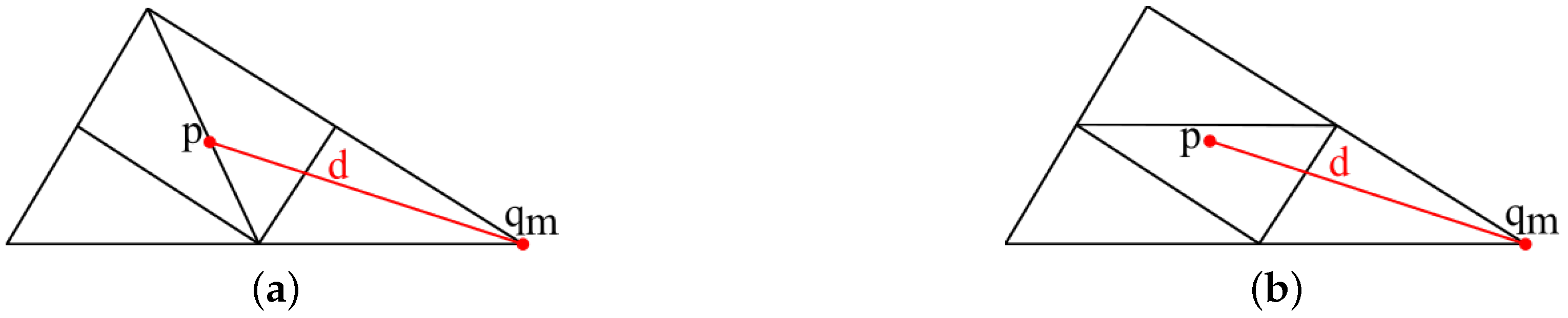
Before describing the theorem, let us first establish some notations and a simple illustration provided in Figure 9. Let p be the representative point of cell C, and be the distance of p to the feature F. As demonstrated in Figure 9, where is the closest point of feature F to representative point p. During the hierarchical traversal of cells, we must evaluate where q is the representative point of a descendant cell of C. Obviously, the closest point can be different from . However, when p and q are close, the search space of becomes a small subset of F. Theorem 1 reduces the search space of the by providing a bound for this space.
Theorem 1.
Given an arbitrary shaped cell C, its representative point p, its distance to feature , and q, the representative point of a descendant cell of C, the search space of is all the edges of the F inside of a circle centered at p with radius , where d is the distance of the farthest possible q to p.
Based on the Theorem 1, it is guaranteed that the closest point to any point in the highlighted triangle in the Figure 9, is inside the bounding circle (the green circle).
Proof of Theorem 1.
Based on the definition of the and we have (see Figure 9):
Otherwise, is closer to q than , and it contradicts with the assumption that is the closest point of the feature to q. Using triangle inequality we have:
To find the search space of in respect to p, using triangle inequality, we have:
and then using (3) we obtain:
□
Figure 10 shows examples of d in triangular grids with congruent refinements with assumption that p is the centroid of the shapes. When d is a small value, the search space is smaller and the resulting algorithm becomes faster. The value of d depends on the shape of the cell and the refinement used in DGGS. In general, . For congruent refinements, d can simply determined using the parent cell’s geometry (i.e., is a point on the boundary of the cell C). For non-congruent refinements, d can be determined with a similar method using the footprint of the cell C. For example, Kevin Sahr [32] provides such a footprint for non-congruent aperture 3 hexagonal tree system. Based on [32], the r shown in Figure 11 covers the entire footprint of the ancestor cell. Therefore, this radius can be used as d.
4. Calculating Distance Transform on DGGS
In this section, we introduce two algorithms that calculate a distance transform on a DGGS grid. The basic idea is presented in the first algorithm and the second algorithm is a modification of the first algorithm which repeats the first algorithm to gain more efficiency. We make use of Theorem 1 to describe the first algorithm as follows.
4.1. Single Stepping from Base to Target Resolution
To calculate DT on a DGGS, we start from a coarse resolution (i.e., base resolution). Once in this resolution, computing distance using the exhaustive search algorithm becomes very quick. Therefore, for each cell we check the distance to all edges of the feature and find the minimum. After finding DT in the base resolution, we compute the bounding circle for each cell in it. We then find and store all the edges of the feature that are within this circle; we call this list of edges the “candidate list” of the cell. Based on Theorem 1, we refine the grid to the target resolution and use the stored candidate lists for DT computation of child (or descendant) cells. Therefore, in the target resolution, we simply need to check the distance from each cell to the edges of the feature that are stored in their parents’ (or ancestors’) candidate list. This process is presented in Algorithm 1. The pseudocode shows how this algorithm can be implemented in three steps: (1) calculating the bounding circles and the candidate lists in the base resolution (lines 1–5), (2), refining the base cells to get the target cells with a jump from the base resolution to the target resolution (lines 6–9), and (3) calculating the distances in the target resolution based on the candidate lists (lines 10–13).
| Algorithm 1 Compute Distance Transform. |
|
Based on Theorem 1, the candidate list calculated in the base resolution is valid for all descendants of the base resolution. This enables us to jump from the base resolution to the target resolution. However, in the next section, we show how it is preferable to refine the mesh one resolution at a time in order to fully exploit the hierarchy. Algorithms 2 and 3 show the details of the and subroutines, respectively. The implementation of the subroutine is given in Appendix A.
| Algorithm 2 Compute Candidate List. |
|
| Algorithm 3 Compute Distance. |
|
4.2. Iterative Refinement
In Section 4.1, we discussed how this algorithm is done in a single step from the base resolution to the target resolution. However, this process can be repeated iteratively between the base and the target resolutions to make the candidate lists smaller (i.e., reduce the search space) step-by-step. The algorithm for this modification is presented in Algorithm 4. The basic idea is to go through the grid from the base resolution and refine the grid one resolution at a time to reach the target resolution. This way, we can refine the candidate lists iteratively in each step. Line 2 of Algorithm 4 is the main loop that controls iterations of the algorithm. Lines 3–20 of this algorithm are similar to Algorithm 1 with a small difference in Algorithm 1’s first step. To calculate the candidate lists, if it’s the first time we are calculating, there is no previous candidate list and no previous distance field (Lines 4–6). The next times, we use the previous candidate list and filter this list to make smaller lists for the next resolution (Lines 7–10).
| Algorithm 4 Compute Distance Transform with Iterative Refinement. |
|
5. Results and Discussion
The proposed DT algorithm works with any DGGS grid regardless of the shape of the cells. To test and benchmark the algorithm, we have implemented it on a Disdyakis Triacontahedron DGGS [26]. The cells of this DGGS are triangular cells with one-to-four congruent refinement as shown in Figure 5. First, we show some visualizations of the output of DT. Then, we describe some tests to evaluate the correctness and performance of our algorithm.
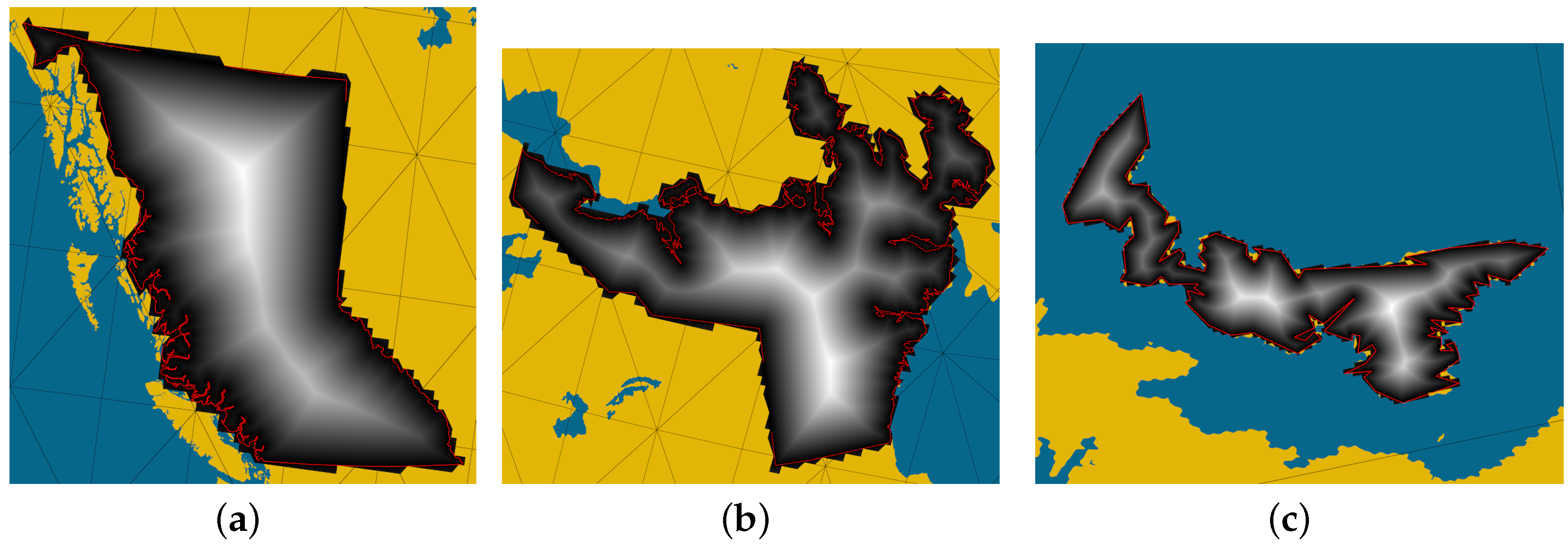
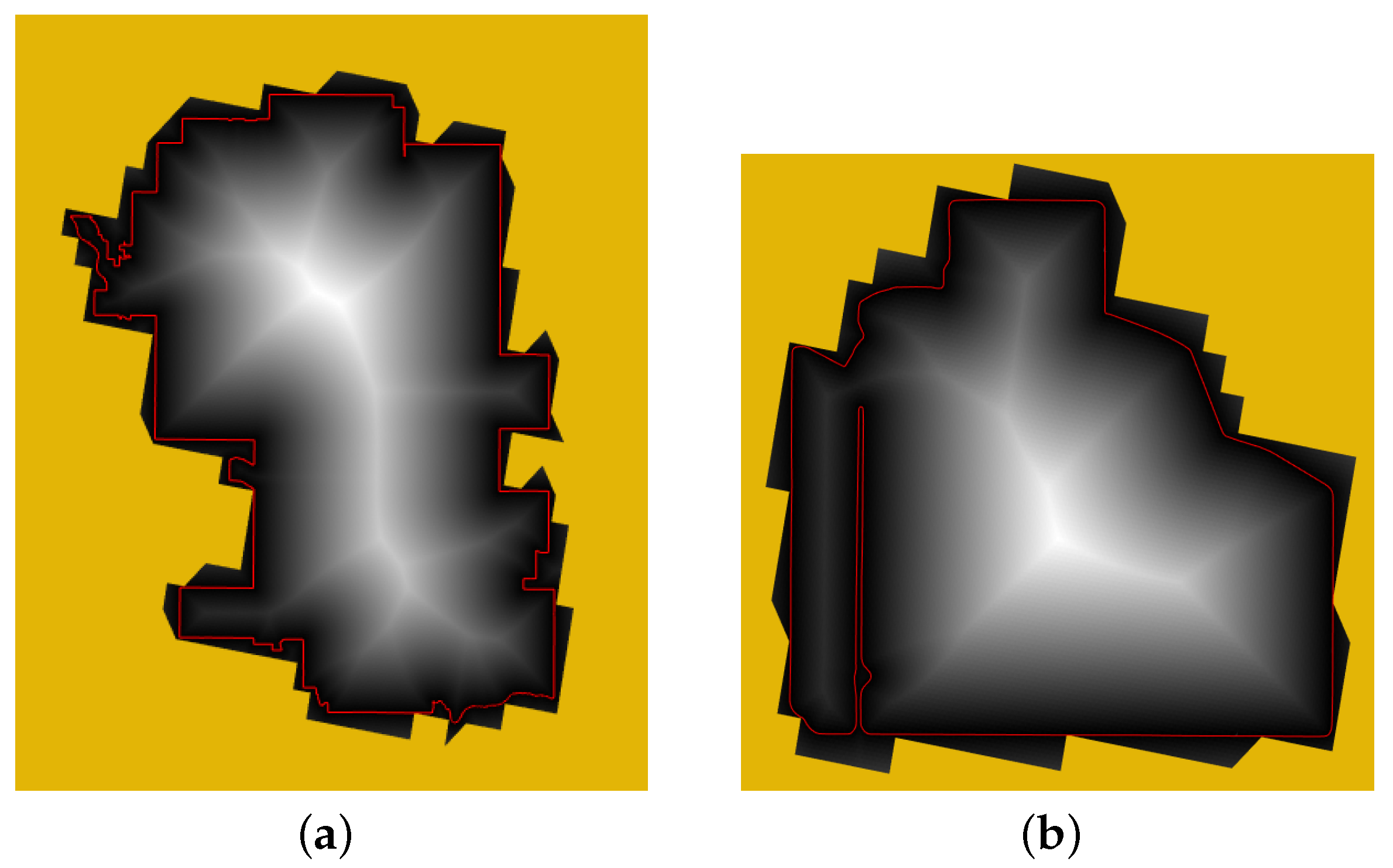
Figure 12 shows a visualization of DT for Ontario at different target resolutions and Figure 13 shows a visualization for three other provinces or territories of Canada. Figure 14 shows the result of DT for two smaller scale features, the border of the city of Calgary and a farm field in Alberta.
5.1. Correctness Analysis
In Section 4.1 and Section 4.2, we discussed the correctness of Algorithms 1 and 4, which both rely on Theorem 1 to reduce the search space by using the hierarchical properties of a DGGS. In this section, we introduce an empirical test which provides further evidence for the correctness of Algorithms 1 and 4. As the ground truth we use the result of the “Generate Near Table” tool from the proximity tools of ArcGIS Pro with the geodesic distance option. To use this tool, we output two pieces of information from our software, (1) the midpoints of the cells used for our DT calculations, and (2) the feature (or boundary) from which the distance is measured. Our system considers line segments of the feature as great-circle arcs, while this is not the case for ArcGIS Pro. To address this issue, we construct a high resolution sampling from the features’ line segments (i.e., 10 m distance between sample points). At this scale, there is practically no difference between a great-circle arc and a straight line. We then import these two pieces of information into ArcGIS Pro with the spatial reference system EPSG:4047 to match our DGGS earth model. We repeated this test for features at three different scales which are shown in Figure 15.
The “Generate Near Table” tool outputs the geodesic distance from each point to the boundary. Using this data, we calculate the difference from the distances we calculated for these points using Algorithms 1 and 4. Table 1 presents the extents of the calculated difference.
Table 1 shows the accuracy of our algorithms and demonstrates that our main algorithms, implementation of all subroutines, and results are correct. It also shows that when identical points are given, both Algorithms 1 and 4 produce the exact same distance. The small difference between ArcGIS Pro and our algorithm might be caused by boundary resampling or floating point errors.
5.2. Performance Analysis
To analyze performance, we use the boundary of the province Ontario of Canada as the input feature which has 449 edges. In the process of this algorithm, DGGS operations are used to obtain vertex positions of a cell (used to find representative point of a cell and also to calculate d), and children of a cell. In addition, operations to project a point from the polyhedral domain of a DGGS to the spherical domain (used in lines 1–3 of Algorithm A1). The aim of the proposed algorithm is to be efficient with the assumption that DGGS operations are efficient. In the other words, this algorithm tries to be efficient by minimizing the number of distance calculation operations needed to compute the distance field. Therefore, to evaluate the algorithm independent of the efficiency of DGGS operations, we calculate and report the number of distance calculation operations performed for each run of the algorithm.
The distance calculation operation or Algorithm A1, calculates the minimum spherical distance from a point to a great circle arc. This is the unit of work and our algorithm tries to minimize the number of occurrences of this operation. The baseline is that we do not exploit the hierarchy of the DGGS and directly use the target resolution to calculate the distance. To achieve this, for each cell in target resolution, we check the distance from the cell to all of the feature edges. Therefore, the total number of operations is the number of cells in target resolution times the number of edges of the feature. In theory, the ideal scenario is that for each cell in the target resolution, we know exactly which edge is the closest and compute the distance of the cell only to that edge. In this case, the total number of operations is only the number of cells in target resolution. Figure 16 showcases the dramatic improvement in the performance of our algorithms explained in Section 4.1 and Section 4.2 compared to the baseline which makes it possible to calculate DT for higher resolutions.
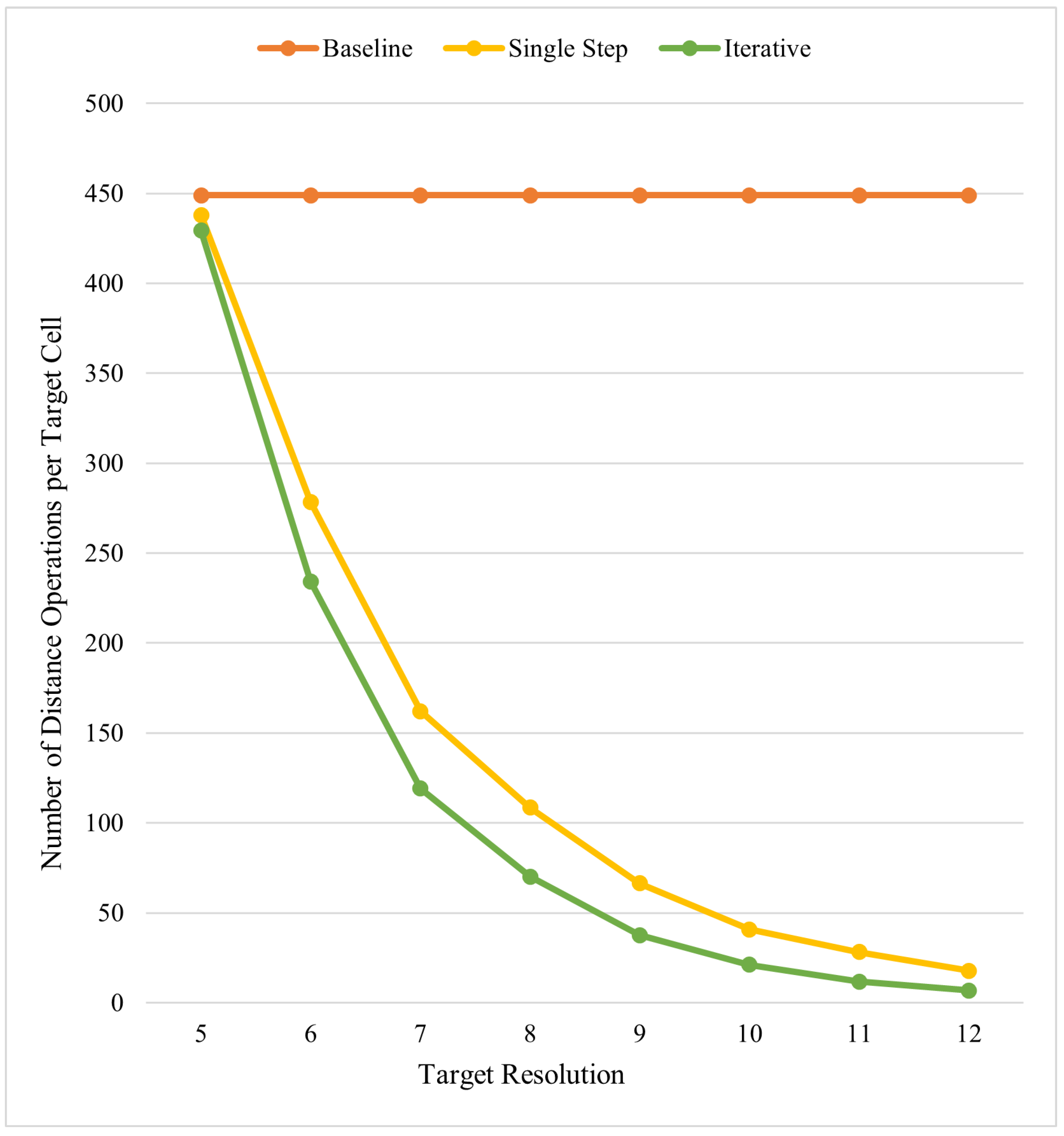
The graphs in Figure 16 are exponential because the number of target cells grows exponentially with the target resolution. To better understand the efficiency of our algorithm, we can slightly change our metric. Figure 17 shows the performance of the algorithms in another metric, reporting the total number of operations per target cell. The domain of this metric is between one (being our ideal scenario of knowing the closest edge to each cell exactly) and the number of edges of the feature (449 for the border of Ontario). The closer this number is to one, the better the performance.
Interestingly, this metric is a constant for the baseline algorithm due to us checking every edge of the feature for each cell at the target resolution. What’s more is that as we observe higher resolutions we can better exploit the hierarchy and get closer to the ideal of 1 operation per target cell.
Based on the analysis presented in this section, the iterative algorithm outperforms the first algorithm. For the boundary of the province of Ontario and the target resolution of 12, the best number of operations per target cell we could achieve using the first algorithm is 17.7. However, using the iterative algorithm with the same inputs, we can achieve 6.9 operations per target cell, which is considerably lower.
5.3. Discussion
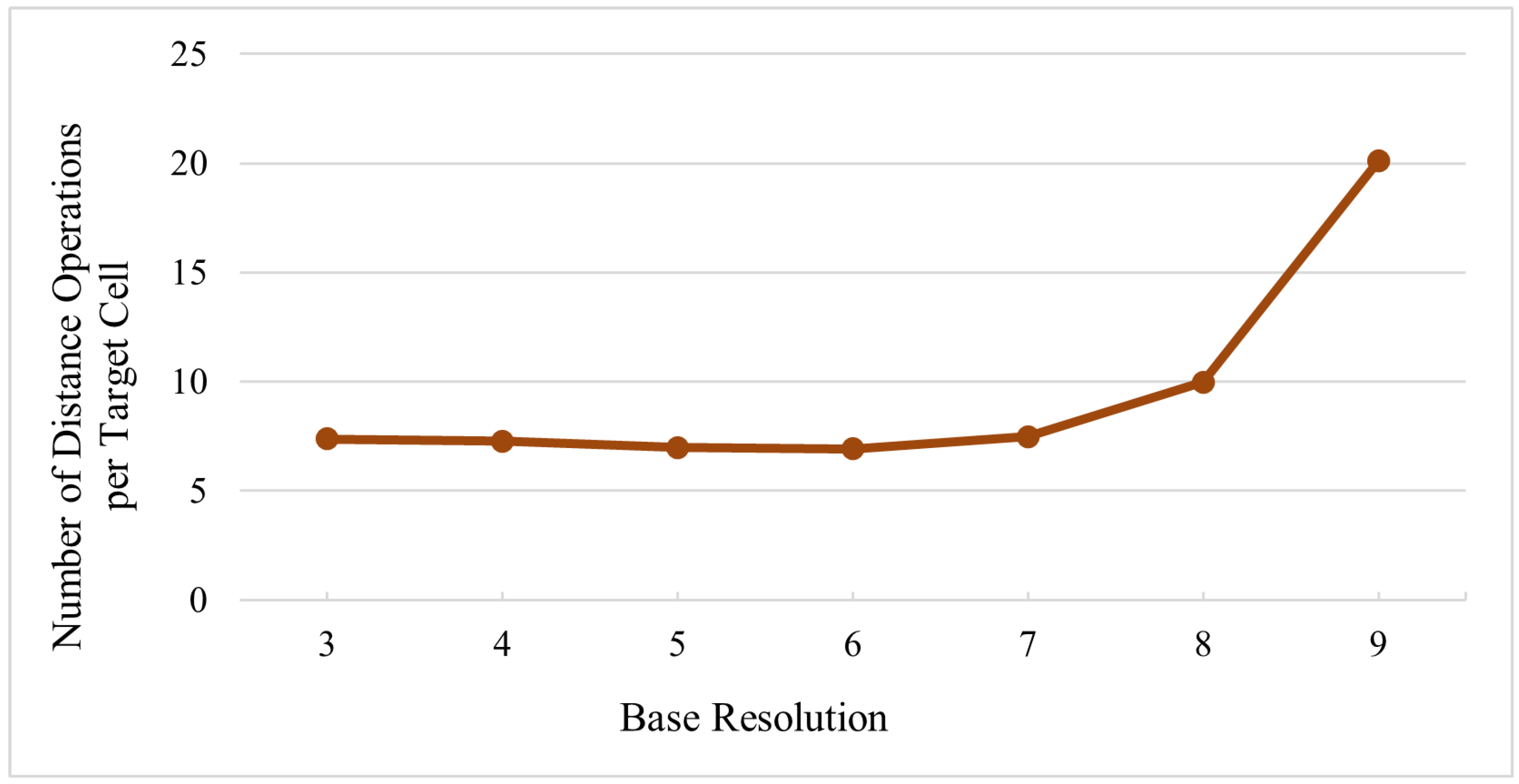
For a specific target resolution, the base resolution is an input to our algorithm that does not affect the result but gives us greater freedom of choice. We previously discussed that this should be a coarse resolution, but a concrete number has not been stated. Figure 18 shows the number of operations used to calculate DT in resolution 12 using the iterative algorithm from different base resolutions. We observe that the number of operations almost strictly increases with increasing the base resolution. However, there is no considerable difference between the base resolutions 3 to 7 (minimum of 6.9 operations and maximum of 7.5 operations). It is clear that if the resolution of the base is very close to the target resolution, we do not gain a large improvement. In addition, our algorithm is not sensitive to this input as long as a coarse resolution is chosen.
The single-step algorithm calculates the candidate lists only in the base resolution first and then jumps to the target resolution. The iterative algorithm on the other hand, after calculating the candidate lists in the base resolutions, refines the candidate lists in every resolution in between. These two algorithms act as extremes, meaning other options are also possible. We have investigated all the combinations possible to reach from the base resolution to the target resolution. We found that always visiting the every resolution in between, like the iterative algorithm does, is always the most efficient.
6. Comparison
Distance transform methods used in traditional GIS that are based on image space introduce distortions. Figure 19a shows the distance transform computed in ArcGIS Pro software using image-based methods, and the distortions can be clearly seen. Figure 19b and Figure 19c show a visualization calculated on the DGGS with our method.
To quantify the amount of distortion caused by traditional GIS (i.e., flat map projections), we performed a test which is similar to Section 5.1. We use the same features as Figure 15, but we switch to the planar distance option within the “Generate Near Table” tool. To use the planar distance calculations, we first project the boundary and the sample points using the WGS 1984 UTM projected coordinate system. Table 2 shows the comparison between the ArcGIS Pro planar distance calculation and the distances produced by Algorithm 4. As we expect, significant distance distortion is present in the planar setting and it reduces to smaller amounts as the scale decreases. In this test, if the feature was not contained in a single UTM zone, we projected all points to the zone that contains the largest portion of the feature. Specifically, we used UTM zone 17N for Ontario, 11N for Calgary, and 12N for the farm field.
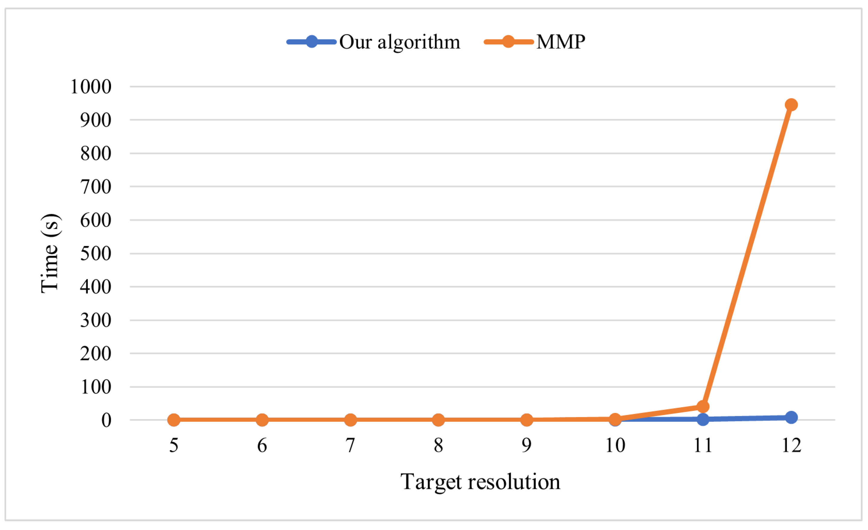
To compare the MMP algorithm [30] for general meshes with our method, there are two aspects to consider. First, the MMP algorithm gives the exact geodesic distance on the mesh. In the case of a DGGS, the mesh is an approximation of a sphere, and points must be projected from the sphere onto the face of the mesh. The MMP algorithm does not consider the effects of the projection and thus its geodesic calculations will not be the same as those calculated on the sphere. However, for higher resolutions of the DGGS, where the mesh is closer to the surface of the sphere, the MMP algorithm becomes a closer approximation to the spherical geodesic distances. Second, the MMP algorithm is less efficient than our algorithm for higher resolutions. For this comparison, we have used the border of Ontario to benchmark the algorithms, the process of which is done on a computer with an Intel Core i7-6700 CPU with both algorithms being tested under the same conditions using the Google Benchmark tool. Figure 20 then compares the execution time of the two algorithms, and Table 3 lists the number of target cells at different resolutions next to their respective execution times. In resolutions lower than 9, the MMP algorithm is faster (though it is less accurate), but the difference is negligible. As we go to higher resolutions and greater numbers of target cells, the MMP algorithm takes more time than our method by a wide margin.
7. Conclusions and Future Work
With the immense amount of data becoming available, distance transform as a tool to analyse such data is important. The problem of distance transform is a solved problem in image processing, but for the geospatial data, image-based methods are unfit. The fast growing new approach of GIS, DGGS, as a tool to better integrate and analyse such data, needs distance transform. To this end, we have proposed a complete and comprehensive method for efficiently calculating the distance transform on top of a DGGS grid. Our approach properly accommodates any potential DGGS regardless of the shape of the grid cells and the congruency of the refinement scheme. We have discussed how to fine-tune the parameters of our algorithm to get the best results for the border of Ontario as input feature. We have also compared our method with the image-based methods and general mesh methods. The comparison shows that our method is superior in terms of accuracy and efficiency for large datasets.
There is still some important future work to be conducted. Our method calculates the distance based on a spherical great-circle arc calculation. Despite most of the DGGSs that use a sphere for their reference model of the Earth, some other DGGSs use an oblate spheroid to provide a more accurate representation. We suspect that our method is applicable to such DGGSs if one can define an efficient distance calculation method for the ellipsoid. However, further research is required to prove this claim.
Another interesting active branch of DGGS research is 3D DGGSs. There exist some works that aim to build a 3D DGGS or extend current 2D DGGSs to 3D DGGS [34,35]. For this work, we have assumed a 2D DGGS, but the same idea might be able to be reimplemented for a 3D DGGS. The initial idea is to prove Theorem 1 for 3D shapes using a bonding sphere instead of a bounding circle, and use this new theorem to build the algorithm. Although, more research is required to evaluate this idea and make any potential necessary changes to the algorithm.
Author Contributions
Conceptualization, Meysam Kazemi and Faramarz Samavati; methodology, Meysam Kazemi and Faramarz Samavati; software, Meysam Kazemi and Lakin Wecker; validation, Meysam Kazemi and Lakin Wecker; formal analysis, Meysam Kazemi and Faramarz Samavati; data curation, Meysam Kazemi and Lakin Wecker; writing—original draft preparation, Meysam Kazemi; writing—review and editing, Meysam Kazemi and Lakin Wecker and Faramarz Samavati; visualization, Meysam Kazemi and Lakin Wecker; supervision, Faramarz Samavati; project administration, Faramarz Samavati; funding acquisition, Faramarz Samavati. All authors have read and agreed to the published version of the manuscript.
Funding
This work was supported by the Natural Sciences and Engineering Research Council (NSERC) of Canada (Grant No. DG 2018-03935).
Institutional Review Board Statement
Not applicable.
Informed Consent Statement
Not applicable.
Data Availability Statement
Not applicable.
Acknowledgments
Special thanks to all members of the GIV research team at the University of Calgary for insights and discussion. Thanks to Kian Samavati for proofreading and grammatical suggestions.
Conflicts of Interest
The authors declare no conflict of interest.
Abbreviations
The following abbreviations are used in this manuscript:
| GIS | Geographic Information System |
| DGGS | Discrete Global Grid System |
| DT | Distance Transform |
Appendix A
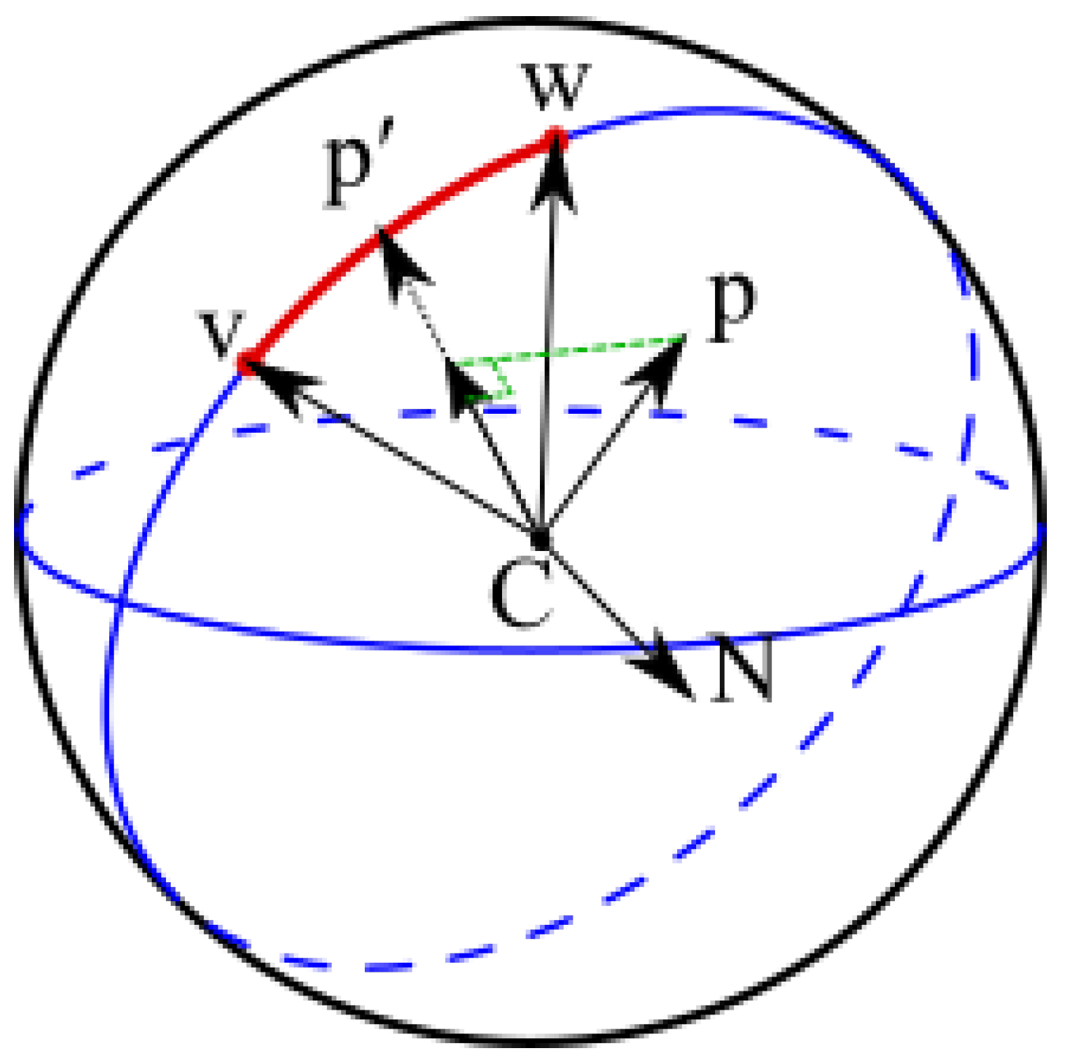
Algorithm A1 shows how one can calculate the distance of a point to a great-circle arc. This algorithm is used in Algorithms 2 and 3. In this algorithm the arc is represented with the two endpoints which are connected to each other with a great-circle arc. It is assumed that the point and the two end points are on the polyhedral domain of the DGGS, so the first step is to project them into the spherical domain.
Figure A1 gives some geometric context. We assume a unit sphere. Vectors and form a plane. The vector is the normal to that plane. We project the point p to that plane. Then, by normalizing that projected vector, we push it to the great-circle that intersects v and w (this is and line 6 in Algorithm A1). So, lies on the great-circle, but we do not know if is between v and w (on the arc) or outside of it. We test it by calculating the cross vectors and . The result of these crosses are also normals to the aforementioned plane. If the cross vectors point in different directions ( angle between them), then is between v and w, otherwise ( angle between them), is outside of them.
| Algorithm A1 Point To Great-circle Arc Distance. |
|
Figure A1.
The red line is the great-circle arc connecting points v and w, and point p is the point in question.
Figure A1.
The red line is the great-circle arc connecting points v and w, and point p is the point in question.

References
- de Smith, M.J. Distance transforms as a new tool in spatial analysis, urban planning, and GIS. Environ. Plan. B Plan. Des. 2004, 31, 85–104. [Google Scholar] [CrossRef]
- Kjaernested, S.N.; Jonsson, M.T.; Palsson, H. Methodology for pipeline route selection using the NSGA II and distance transform algorithms. In Proceedings of the International Design Engineering Technical Conferences and Computers and Information in Engineering Conference, Washington, DC, USA, 28–31 August 2011; Volume 54822, pp. 543–552. [Google Scholar]
- Kristinsson, H.; Jonsson, M.T.; Jónsdóttir, F. Pipe route design using variable topography distance transforms. In Proceedings of the International Design Engineering Technical Conferences and Computers and Information in Engineering Conference, Long Beach, CA, USA, 24–28 September 2005; Volume 4739, pp. 331–336. [Google Scholar]
- Pu, H.; Zhang, H.; Li, W.; Xiong, J.; Hu, J.; Wang, J. Concurrent optimization of mountain railway alignment and station locations using a distance transform algorithm. Comput. Ind. Eng. 2019, 127, 1297–1314. [Google Scholar] [CrossRef]
- ArcGIS. Euclidean Distance. 2021. Available online: https://desktop.arcgis.com/en/arcmap/latest/tools/spatial-analyst-toolbox/euclidean-distance.htm (accessed on 17 June 2021).
- Mahdavi-Amiri, A.; Alderson, T.; Samavati, F. A survey of digital earth. Comput. Graph. 2015, 53, 95–117. [Google Scholar] [CrossRef]
- Alderson, T.; Purss, M.; Du, X.; Mahdavi-Amiri, A.; Samavati, F. Digital earth platforms. In Manual of Digital Earth; Springer: Singapore, 2020; pp. 25–54. [Google Scholar]
- Goodchild, M.F. Reimagining the history of GIS. Ann. GIS 2018, 24, 1–8. [Google Scholar] [CrossRef]
- Bommes, D.; Kobbelt, L. Accurate Computation of Geodesic Distance Fields for Polygonal Curves on Triangle Meshes; VMV: Saarbrücken, Germany, 2007; Volume 7, pp. 151–160. Available online: https://www.graphics.rwth-aachen.de/publication/63/bommes_07_VMV_011.pdf (accessed on 17 June 2021).
- Crane, K.; Weischedel, C.; Wardetzky, M. The Heat Method for Distance Computation. Commun. ACM 2017, 60, 90–99. [Google Scholar] [CrossRef]
- Rosenfeld, A.; Pfaltz, J.L. Sequential operations in digital picture processing. J. ACM 1966, 13, 471–494. [Google Scholar] [CrossRef]
- Cuisenaire, O. Distance Transformations: Fast Algorithms and Applications to Medical Image Processing; Technical Report; UCL: Louvain-la-Neuve, Belgium, 1999; Available online: https://infoscience.epfl.ch/record/61606 (accessed on 17 June 2021).
- Wang, Y.; Wei, X.; Liu, F.; Chen, J.; Zhou, Y.; Shen, W.; Fishman, E.K.; Yuille, A.L. Deep distance transform for tubular structure segmentation in ct scans. In Proceedings of the IEEE/CVF Conference on Computer Vision and Pattern Recognition, Seattle, WA, USA, 14–19 June 2020; pp. 3833–3842. [Google Scholar]
- Liu, H.C.; Srinath, M.D. Partial shape classification using contour matching in distance transformation. IEEE Trans. Pattern Anal. Mach. Intell. 1990, 12, 1072–1079. [Google Scholar] [CrossRef]
- Lavallée, S.; Szeliski, R. Recovering the position and orientation of free-form objects from image contours using 3D distance maps. IEEE Trans. Pattern Anal. Mach. Intell. 1995, 17, 378–390. [Google Scholar] [CrossRef]
- Teixeira, R.C. Curvature Motions, Medial Axes and Distance Transforms; Harvard University: Cambridge, MA, USA, 1998; Available online: https://www.proquest.com/openview/50c844f9001964e3be3073ae12a738ad/1?pq-origsite=gscholar&cbl=18750&diss=y (accessed on 17 June 2021).
- Moustakas, K.; Tzovaras, D.; Strintzis, M.G. SQ-Map: Efficient layered collision detection and haptic rendering. IEEE Trans. Vis. Comput. Graph. 2006, 13, 80–93. [Google Scholar] [CrossRef]
- Choi, Y.H.; Lee, T.K.; Baek, S.H.; Oh, S.Y. Online complete coverage path planning for mobile robots based on linked spiral paths using constrained inverse distance transform. In Proceedings of the 2009 IEEE/RSJ International Conference on Intelligent Robots and Systems, St. Louis, MO, USA, 10–15 October 2009; pp. 5788–5793. [Google Scholar]
- Acharjya, P.; Sinha, A.; Sarkar, S.; Dey, S.; Ghosh, S. A new approach of watershed algorithm using distance transform applied to image segmentation. Int. J. Innov. Res. Comput. Commun. Eng. 2013, 1, 185–189. [Google Scholar]
- Ma, J.; Wei, Z.; Zhang, Y.; Wang, Y.; Lv, R.; Zhu, C.; Gaoxiang, C.; Liu, J.; Peng, C.; Wang, L.; et al. How distance transform maps boost segmentation CNNs: An empirical study. In Medical Imaging with Deep Learning; PMLR Press: Cambridge, MA, USA, 2020; pp. 479–492. Available online: https://proceedings.mlr.press/v121/ma20b.html (accessed on 17 June 2021).
- Lee, Y.H.; Horng, S.J. Fast parallel chessboard distance transform algorithms. In Proceedings of the 1996 International Conference on Parallel and Distributed Systems, Tokyo, Japan, 3–6 June 1996; pp. 488–493. [Google Scholar]
- Lee, Y.H.; Horng, S.J. Optimal computing the chessboard distance transform on parallel processing systems. Comput. Vis. Image Underst. 1999, 73, 374–390. [Google Scholar] [CrossRef]
- Butt, M.A.; Maragos, P. Optimum design of chamfer distance transforms. IEEE Trans. Image Process. 1998, 7, 1477–1484. [Google Scholar] [CrossRef]
- Fabbri, R.; Costa, L.D.F.; Torelli, J.C.; Bruno, O.M. 2D Euclidean distance transform algorithms: A comparative survey. ACM Comput. Surv. (CSUR) 2008, 40, 1–44. [Google Scholar] [CrossRef]
- Schmaltz, T.; Melnitchouk, A. Variable Zone Crop-Specific Inputs Prescription Method and Systems Therefor. U.S. Patent CA 2,663,917, December 2014. [Google Scholar]
- Hall, J.; Wecker, L.; Ulmer, B.; Samavati, F. Disdyakis triacontahedron DGGS. ISPRS Int. J.-Geo-Inf. 2020, 9, 315. [Google Scholar] [CrossRef]
- Ciesielski, K.C.; Chen, X.; Udupa, J.K.; Grevera, G.J. Linear time algorithms for exact distance transform. J. Math. Imaging Vision 2011, 39, 193–209. [Google Scholar] [CrossRef]
- Shih, F.Y.; Wu, Y.T. Fast Euclidean distance transformation in two scans using a 3× 3 neighborhood. Comput. Vis. Image Underst. 2004, 93, 195–205. [Google Scholar] [CrossRef]
- Lucet, Y. New sequential exact Euclidean distance transform algorithms based on convex analysis. Image Vis. Comput. 2009, 27, 37–44. [Google Scholar] [CrossRef]
- Mitchell, J.S.; Mount, D.M.; Papadimitriou, C.H. The discrete geodesic problem. SIAM J. Comput. 1987, 16, 647–668. [Google Scholar] [CrossRef]
- Surazhsky, V.; Surazhsky, T.; Kirsanov, D.; Gortler, S.J.; Hoppe, H. Fast exact and approximate geodesics on meshes. ACM Trans. Graph. (TOG) 2005, 24, 553–560. [Google Scholar] [CrossRef] [Green Version]
- Sahr, K. Location coding on icosahedral aperture 3 hexagon discrete global grids. Discrete Global Grids. Comput. Environ. Urban Syst. 2008, 32, 174–187. [Google Scholar] [CrossRef]
- Reprinted from Computers, Environment and Urban Systems, 32, Sahr, K., Location coding on icosahedral aperture 3 hexagon discrete global grids, 186, Copyright 2022, with permission from Elsevier (Licence No. 5246110741204).
- Ulmer, B.; Hall, J.; Samavati, F. General Method for Extending Discrete Global Grid Systems to Three Dimensions. ISPRS Int. J.-Geo-Inf. 2020, 9, 233. [Google Scholar] [CrossRef] [Green Version]
- Ulmer, B.; Samavati, F. Toward volume preserving spheroid degenerated-octree grid. GeoInformatica 2020, 24, 505–529. [Google Scholar] [CrossRef]
Figure 1.
DT applied to different types of grids (a) regular image-based grid, (b) semi-regular Disdyakis Triacontahedron DGGS grid, (c) irregular general mesh. In this visualization, darker cells are closer to the feature and brighter cells are farther to the feature.
Figure 1.
DT applied to different types of grids (a) regular image-based grid, (b) semi-regular Disdyakis Triacontahedron DGGS grid, (c) irregular general mesh. In this visualization, darker cells are closer to the feature and brighter cells are farther to the feature.

Figure 2.
(a) The binary image before applying DT. (b) The result of applying DT to the binary image.
Figure 2.
(a) The binary image before applying DT. (b) The result of applying DT to the binary image.
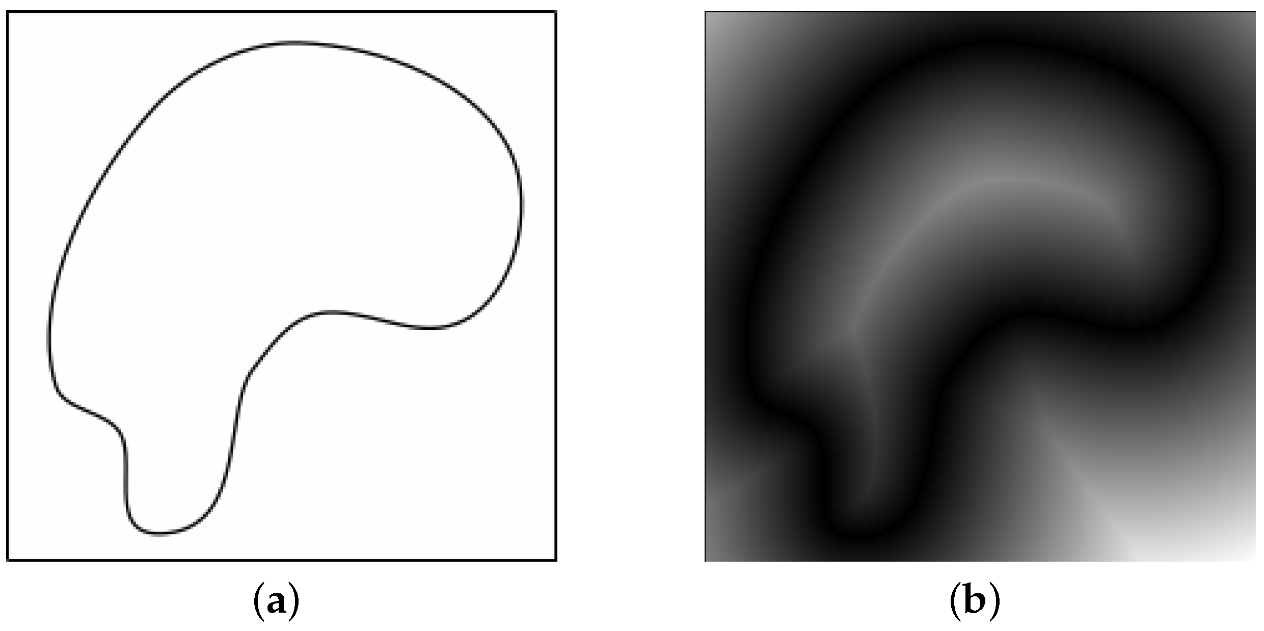
Figure 3.
(a) Tetrahedron (b) Octahedron (c) Icosahedron (d) Disdyakis dodecahedron (e) Disdyakis triacontahedron.
Figure 3.
(a) Tetrahedron (b) Octahedron (c) Icosahedron (d) Disdyakis dodecahedron (e) Disdyakis triacontahedron.
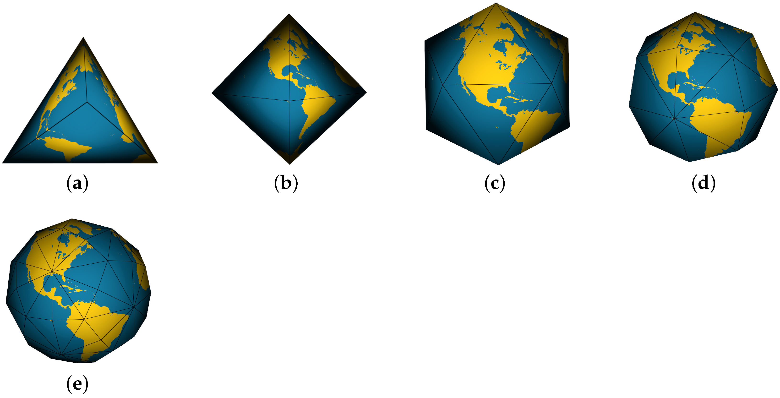
Figure 4.
Examples of congruent (a) 1 to 4 quad, (b) 1 to 3 triangle, and (c) non-congruent hexagonal refinement. The black cells are original cells and the green lines show one level of refinement.
Figure 4.
Examples of congruent (a) 1 to 4 quad, (b) 1 to 3 triangle, and (c) non-congruent hexagonal refinement. The black cells are original cells and the green lines show one level of refinement.

Figure 5.
Disdyakis Triacontahedron DGGS at resolution (a) 1, (b) 2, and (c) 3.
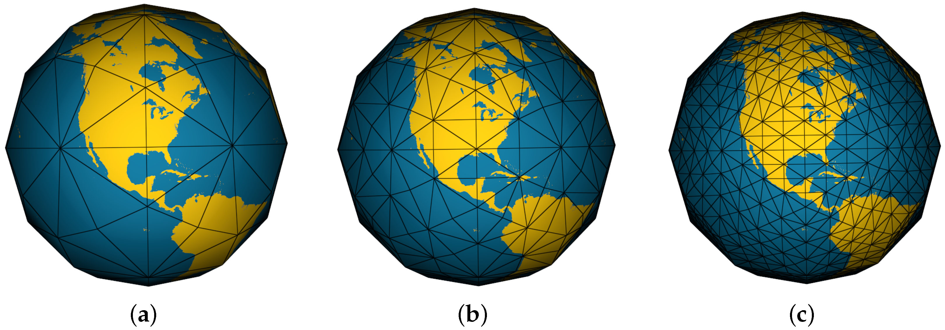
Figure 6.
Disdyakis Triacontahedron DGGS at resolution three in the polyhedral domain (left) and the spherical domain (right).
Figure 6.
Disdyakis Triacontahedron DGGS at resolution three in the polyhedral domain (left) and the spherical domain (right).

Figure 7.
The red line is the great-circle arc connecting points p and q.
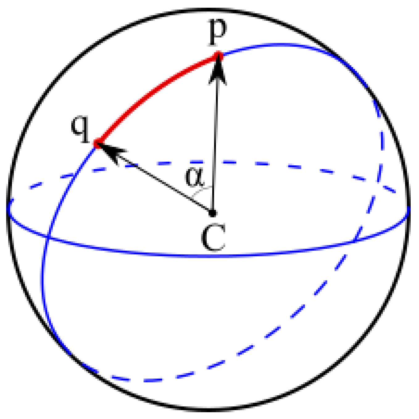
Figure 8.
Distance of a cell to a feature.
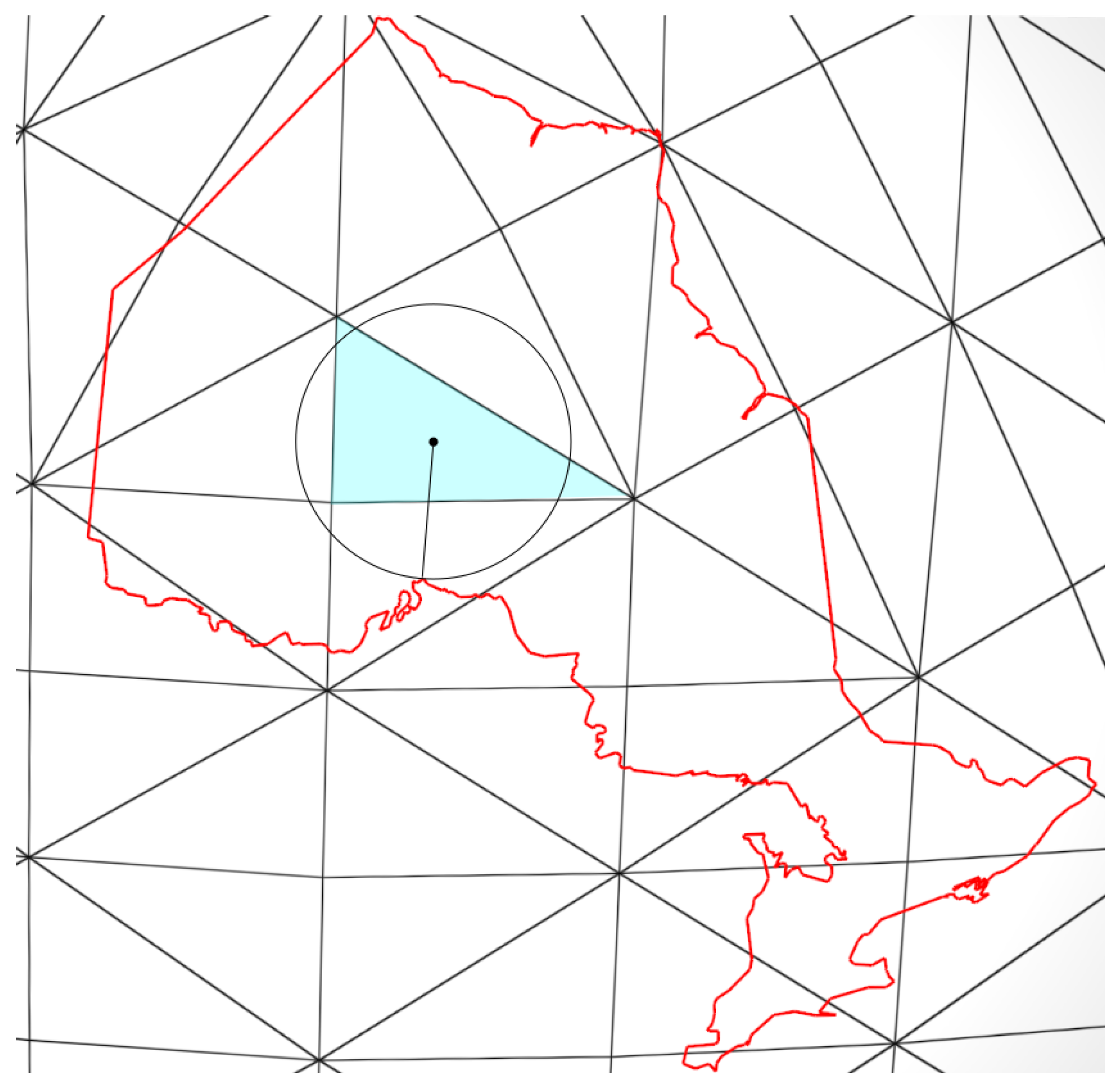
Figure 9.
An example of a the bounding space (green circle).
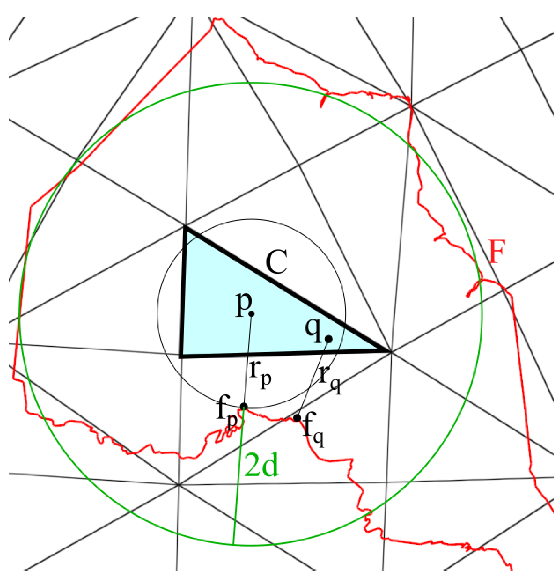
Figure 10.
Two types of triangle 1 to 4 refinements with appropriate d. (a) 1:4 Longest-edge bisection, which is used in [26]. (b) 1:4 midpoint refinement which is a more common refinement.
Figure 10.
Two types of triangle 1 to 4 refinements with appropriate d. (a) 1:4 Longest-edge bisection, which is used in [26]. (b) 1:4 midpoint refinement which is a more common refinement.

Figure 11.
The gray cells are the footprint of the large black hexagon at 4 resolution higher. Image taken Reprinted with permission from Ref. [32] Copyright 2008 Elsevier [33].
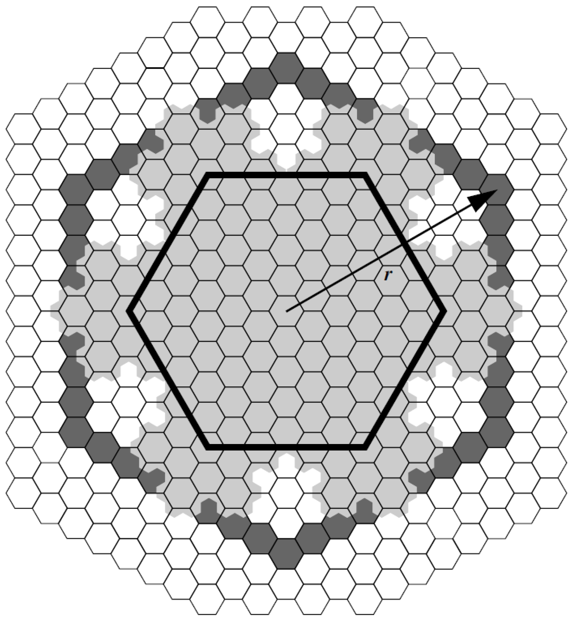
Figure 12.
Distance transform for the border of Ontario at target resolution (a) 7 (Avg. cell size: 1037.3 km), (b) 9 (Avg. cell size: 64.8 km), (c) 12 (Avg. cell size: 1.0 km).
Figure 12.
Distance transform for the border of Ontario at target resolution (a) 7 (Avg. cell size: 1037.3 km), (b) 9 (Avg. cell size: 64.8 km), (c) 12 (Avg. cell size: 1.0 km).
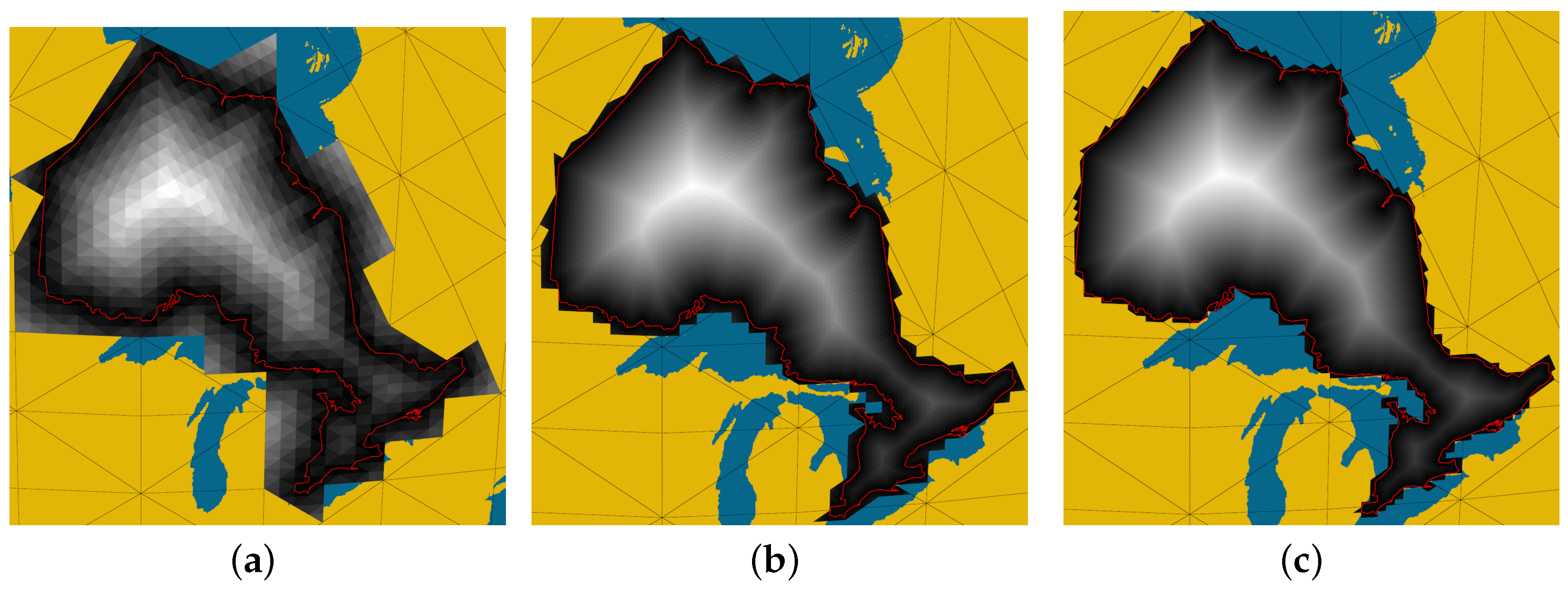
Figure 13.
Distance transform for the border of (a) Mainland British Columbia and (b) Nunavut at target resolution 11 (Avg. cell size: 4.0 km), and (c) Price’s Edward Island at target resolution 15 (Avg. cell size: 0.016 km).
Figure 13.
Distance transform for the border of (a) Mainland British Columbia and (b) Nunavut at target resolution 11 (Avg. cell size: 4.0 km), and (c) Price’s Edward Island at target resolution 15 (Avg. cell size: 0.016 km).

Figure 14.
Distance transform for the border of (a) the city of Calgary at target resolution 15 (Avg. cell size: 0.016 km) and (b) a farm field in Alberta at target resolution 19 (Avg. cell size: 61.8 m).
Figure 14.
Distance transform for the border of (a) the city of Calgary at target resolution 15 (Avg. cell size: 0.016 km) and (b) a farm field in Alberta at target resolution 19 (Avg. cell size: 61.8 m).

Figure 15.
Distance transform sample points and corresponding boundaries imported into ArcGIS Pro for (a) the province of Ontario, (b) the city of Calgary, and (c) a farm field in Alberta.
Figure 15.
Distance transform sample points and corresponding boundaries imported into ArcGIS Pro for (a) the province of Ontario, (b) the city of Calgary, and (c) a farm field in Alberta.
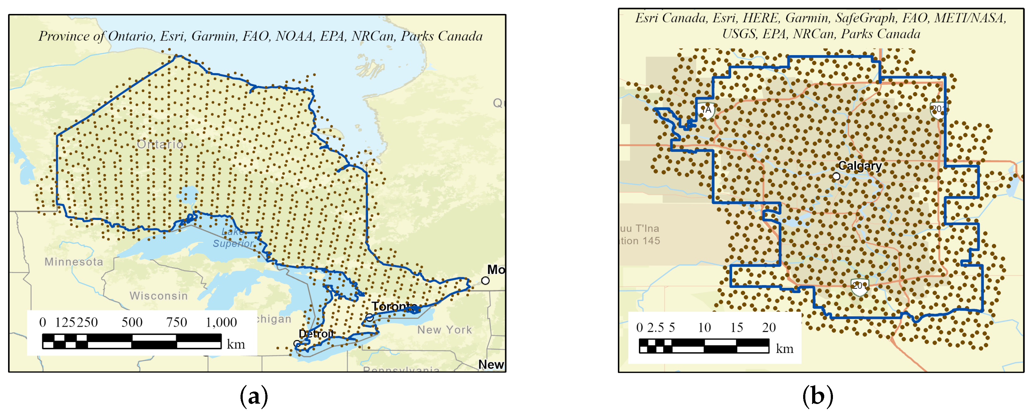
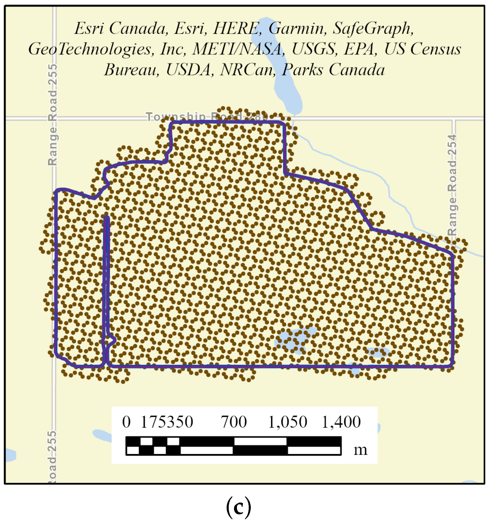
Figure 16.
The number of distance operations in different target resolutions for the boundary of Ontario.
Figure 16.
The number of distance operations in different target resolutions for the boundary of Ontario.
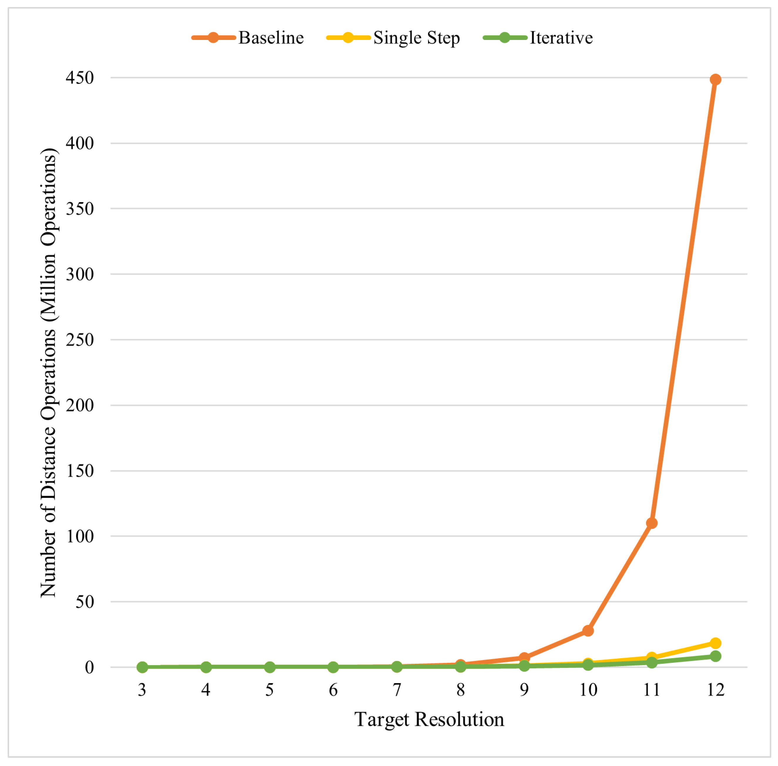
Figure 17.
The number of distance operations in different target resolutions for the boundary of Ontario.
Figure 17.
The number of distance operations in different target resolutions for the boundary of Ontario.

Figure 18.
The effect of the base resolution on the performance of the iterative algorithm for the target resolution 12.
Figure 18.
The effect of the base resolution on the performance of the iterative algorithm for the target resolution 12.

Figure 19.
Distance transform from Yellowknife using (a) ArcGIS and planar distance calculations, (b,c) DGGS and our method.
Figure 19.
Distance transform from Yellowknife using (a) ArcGIS and planar distance calculations, (b,c) DGGS and our method.
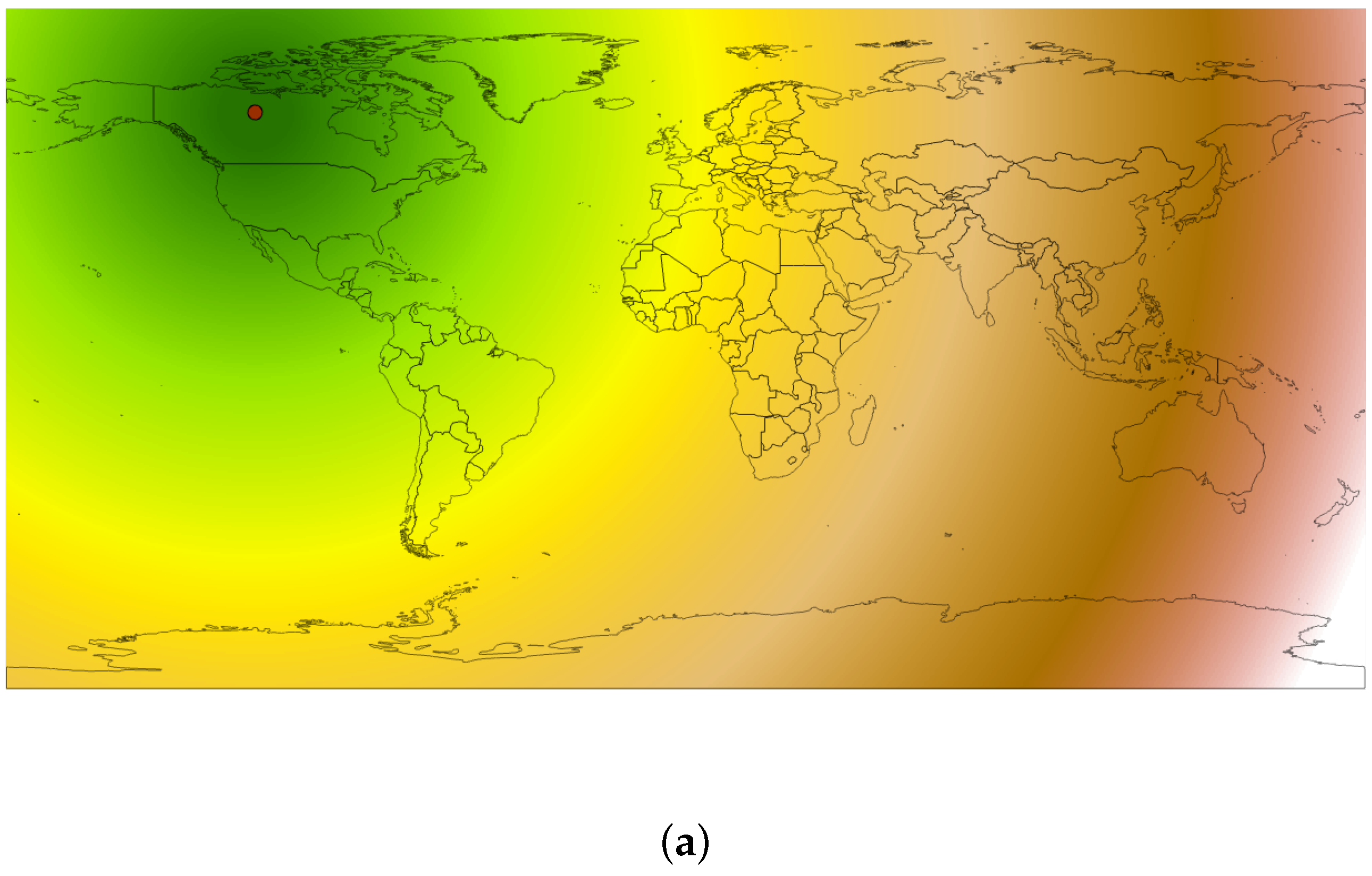
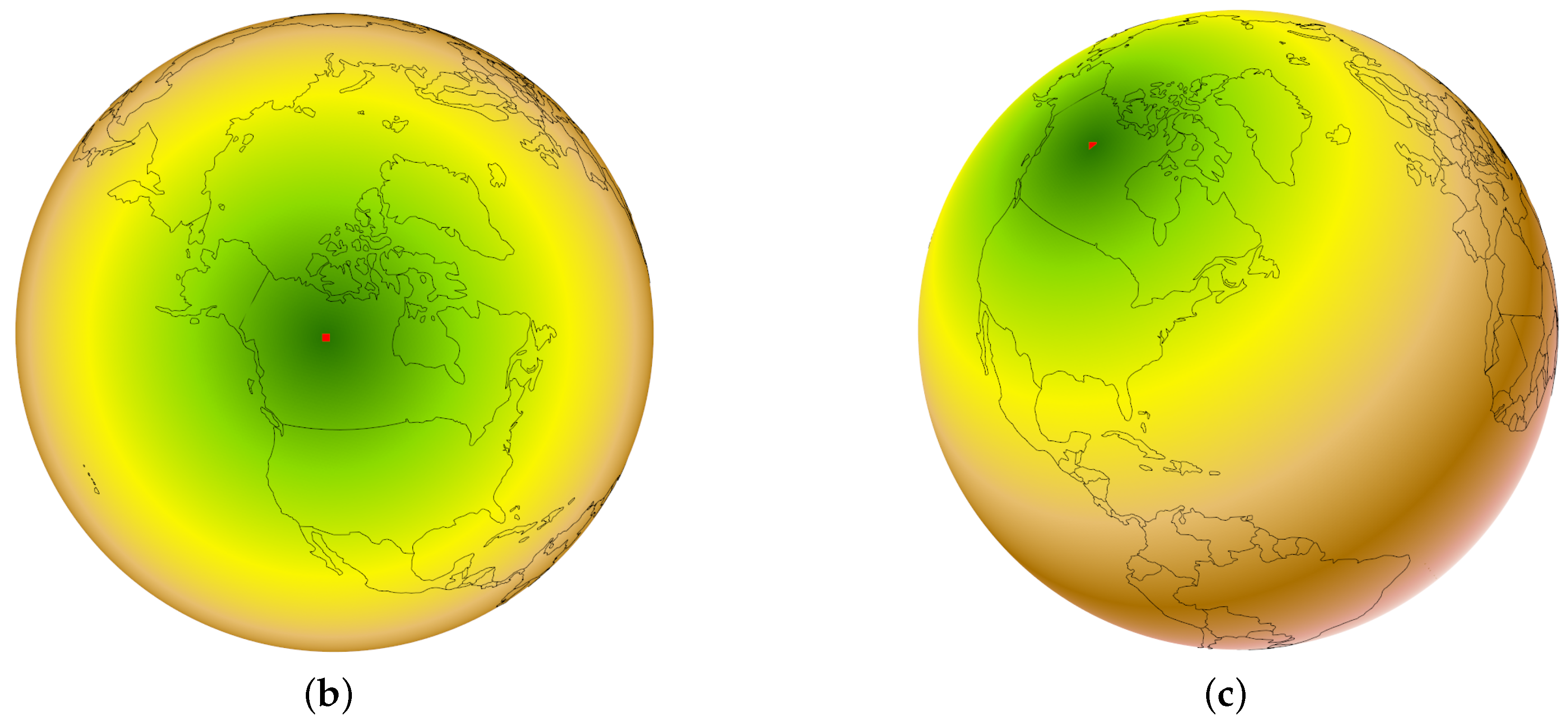
Figure 20.
Execution time of our algorithm and the MMP algorithm at different resolutions for border of Ontario.
Figure 20.
Execution time of our algorithm and the MMP algorithm at different resolutions for border of Ontario.

Table 1.
Difference in millimeters between the ArcGIS Pro calculated geodesic distances and ours.
| Difference | Min (mm) | Max (mm) | Mean (mm) | Std. Deviation (mm) |
|---|---|---|---|---|
| Ontario (Algorithm 1) | 0.0 | 0.0 | 0.0 | 0.0 |
| Calgary (Algorithm 1) | −1.3 | 1.8 | 0.0 | 0.1 |
| Farm field (Algorithm 1) | −6.4 | 11.4 | 0.1 | 0.6 |
| Ontario (Algorithm 4) | 0.0 | 0.0 | 0.0 | 0.0 |
| Calgary (Algorithm 4) | −1.3 | 1.8 | 0.0 | 0.1 |
| Farm field (Algorithm 4) | −6.4 | 11.4 | 0.1 | 0.6 |
Table 2.
Difference in meters between the ArcGIS Pro calculated planar distances and the distances from Algorithm 4.
Table 2.
Difference in meters between the ArcGIS Pro calculated planar distances and the distances from Algorithm 4.
| Difference | Min (m) | Max (m) | Mean (m) | Std. Deviation (m) |
|---|---|---|---|---|
| Ontario | −85.9256 | 3268.89 | 431.938 | 581.674 |
| Calgary | 0.0068 | 32.80 | 6.301 | 6.725 |
| Farm field | −0.0058 | 1.80 | 0.307 | 0.359 |
Table 3.
Execution time of our algorithm and MMP algorithm along with number of target cells for the border of Ontario.
Table 3.
Execution time of our algorithm and MMP algorithm along with number of target cells for the border of Ontario.
| Target Resolution | # of Target Cells | Our Algorithm (ms) | MMP (ms) |
|---|---|---|---|
| 5 | 208 | 74.0 | 0.8 |
| 6 | 464 | 66.6 | 1.6 |
| 7 | 1488 | 113.3 | 5.7 |
| 8 | 5952 | 159.6 | 33.9 |
| 9 | 19,392 | 273.9 | 240.7 |
| 10 | 69,696 | 719.7 | 2474.8 |
| 11 | 260,480 | 2200.3 | 40,178.0 |
| 12 | 1,041,920 | 7541.7 | 946,192.2 |
Publisher’s Note: MDPI stays neutral with regard to jurisdictional claims in published maps and institutional affiliations. |
© 2022 by the authors. Licensee MDPI, Basel, Switzerland. This article is an open access article distributed under the terms and conditions of the Creative Commons Attribution (CC BY) license (https://creativecommons.org/licenses/by/4.0/).
Share and Cite
MDPI and ACS Style
Kazemi, M.; Wecker, L.; Samavati, F. Efficient Calculation of Distance Transform on Discrete Global Grid Systems. ISPRS Int. J. Geo-Inf. 2022, 11, 322. https://doi.org/10.3390/ijgi11060322
AMA Style
Kazemi M, Wecker L, Samavati F. Efficient Calculation of Distance Transform on Discrete Global Grid Systems. ISPRS International Journal of Geo-Information. 2022; 11(6):322. https://doi.org/10.3390/ijgi11060322
Chicago/Turabian StyleKazemi, Meysam, Lakin Wecker, and Faramarz Samavati. 2022. "Efficient Calculation of Distance Transform on Discrete Global Grid Systems" ISPRS International Journal of Geo-Information 11, no. 6: 322. https://doi.org/10.3390/ijgi11060322
Note that from the first issue of 2016, this journal uses article numbers instead of page numbers. See further details here.