Abstract
Spatial information analysis has gained increasing attention in recent years due to its wide range of applications, from disaster prevention and human behavioral patterns to commercial value. This study proposes a novel application to help businesses identify optimal locations for new stores. Optimal store locations are close to other stores with similar customer groups. However, they are also a suitable distance from stores that might represent competition. The style of a new store also exerts a significant effect. In this paper, we utilized check-in data and user profiles from location-based social networks to calculate the degree of influence of each store in a road network on the query user to identify optimal new store locations. As calculating the degree of influence of every store in a road network is time-consuming, we added two accelerating algorithms to the proposed baseline. The experiment results verified the validity of the proposed approach.
1. Introduction
Many studies have applied big data to commercial applications, including helping real estate agents find suitable residential areas for customers [1] and helping companies estimate the number of customers a product may attract based on its characteristics [2]. These applications are enabled by continuous evolution in hardware and computing performance, which allows users to store and compute diverse and massive amounts of spatial and temporal information, such as the locations of the street intersections in a city, the distances between intersections, and the visit records of users. This study discusses a means of utilizing this information to help businesses find suitable locations for new stores. This problem is well-considered in the literature [3,4,5,6]. For example, consider the road network presented in Figure 1, where solid points indicate existing stores and hollow points indicate candidate locations. If user U wants to open a new family restaurant, the target algorithm can assist U to find the best location. The algorithm suggests location A, which is in the middle of a group of family attractions and is far away from other well-known family restaurants. For convenience, existing attractions and stores are referred to as ‘points of interest’ (POIs).
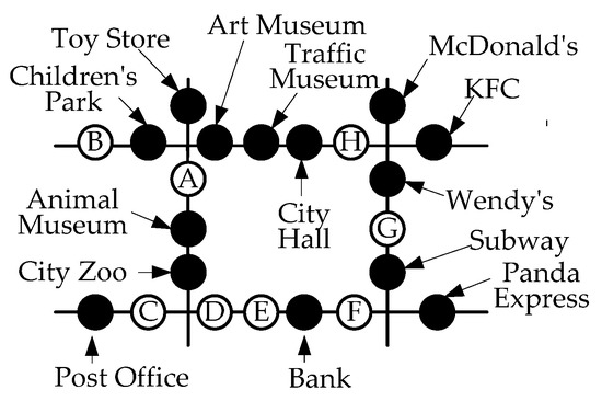
Figure 1.
An example explaining the proposed problem.
Some previous studies have discussed the above issues. For example, Qi et al. [7] and Lee [4] found optimal store locations by minimizing the average Euclidean distance between a customer and the customer’s nearest store. Xiao et al. [3] replaced Euclidean distance with road distance, because this is more intuitive for users of a road network. Lin et al. [5], Sacharidis et al. [6], and Su [8] highlighted that [3,4,7] only consider the impact of positive POIs (i.e., those that attract customers), neglecting the effect of negative POIs (i.e., those that repel customers or represent competitors). As a result, store owners may make critical errors, such as opening a bakery or restaurant next to a junkyard or a home barber next to a trendy hair salon. However, while considering the influence of both positive and negative POIs represents an improvement, the predicted level of influence is usually unrealistic. Previous studies have shown that because the new store is not open at the time of the solution, it is not possible to calculate the level of influence of each POI on the new store. Therefore, these influences can only be set to a fixed value, which leads to inaccuracy.
This paper proposes using location-based social network databases (LBSN datasets) to estimate the influence of positive and negative POIs on the new store. LBSN services enable users to volunteer information (known as user profiles) on LBSN datasets and share the locations that they visit as well as reviews of these locations (known as check-in data). Foursquare [9] and Facebook [10] are good examples. LBSN datasets provide real-world behavioral data and are widely used in a variety of commercial applications [11,12,13]. We propose evaluating the degree of influence of each POI on a customer base of the new store by first asking the query user to identify reference POIs. For example, for a family restaurant, reference POIs might be other family restaurants or children’s playgrounds. The influence of a POI on the new store is defined as the average influence score of that POI with all selected reference POIs. This refines the conventional approach of fixed values for POI influence.
While it increases the accuracy of recommendations, applying LBSN data to the target problem greatly increases the computational cost of the proposed algorithm. Not only must additional data be retrieved from the LBSN dataset, but the influence of each POI must be calculated one by one. Three algorithms are presented in this paper. The first is the baseline algorithm, which introduces the basic concepts to solve the proposed problem. The second and third algorithms are based on the new data structure G+-tree (which represents an extension of G-tree) to reduce the computational cost and accelerate the query speed. The efficiency of the proposed approaches are verified on two simulated datasets and one real dataset.
This paper makes novel contributions to the topic, both conceptually and in terms of algorithm design. Table 1 lists the factors considered in this study: road distance, positive and negative POIs, and the degree of POI influence based on LBSN datasets. Compared with studies that set the degree of influence using a fixed value, the proposed approach is more in line with the real-world needs of users. In terms of algorithm design, we propose the new data structure G+-tree to reduce the computational load introduced by the use of LBSN datasets.

Table 1.
Comparison of related works.
Despite its valuable contributions, this paper is subject to two important limitations. Generally speaking, LBSN data are subject to user bias [16,17,18] and may not always conform to real-world situations. This can create a gap between the solution output by the algorithm and the actual best solution. However, this gap is usually considered permissible, as the LBSN dataset is closer to reality than most other public datasets. Further information is available in [16,17,18]. In addition, customer groups and the proximity to positive and negative POIs are not the only factors affecting the optimal choice of location for a new store. Other important factors include transportation, rent, land use, and licenses. Because the current paper is focused on the novel contribution of including the degree of influence of POI on a customer base for the new store based on LSBN data, these additional factors are considered beyond the scope of this paper. The general approach proposed in this paper could be adapted to include specific variables such as these, by the reader or by future studies.
The remainder of this study is organized as follows. Section 2 reviews the relevant literature, and Section 3 formally defines the problem. Section 4 explains the system framework and details the baseline algorithm. Section 5 presents the area-pruning (AP) algorithm. Section 6 presents the area-and-edge-pruning (AEP) algorithm. Section 7 presents our experiment results, and Section 8 contains our conclusions.
2. Related Work
2.1. Location-Based Social Networks (LBSN Datasets)
LBSN services enable users to share their travel experiences anytime, anywhere via mobile devices. Their experiences are represented by check-in time, the location of the POI visited by the user, and user ID. It also allows for the collection of demographic information such as the age, gender, and educational background of users, usually presented in the form of user profiles. There are numerous applications for such LBSN data. Li et al. [19] and Bao et al. [20] employed check-in data to assist users to find their preferred POIs and help POI owners to attract more customers. Hsieh et al. [21] and Lu et al. [22] recommended personalized trips by mining user’s check-in behaviors. Wen et al. [23] observed that, when planning a trip, users may use keywords to indicate their preferences. They utilized LBSN data to find skylines for travel routes that combine the multi-dimensional measurements (POI attractiveness, proper visiting time, and geographical social influence) of routes.
2.2. Commercial Applications
Arvanitis et al. [2] formulated the concept of product attractiveness based on the notion of reverse skyline queries and helped companies estimate the number of customers a product may attract based on its characteristics. Zhang et al. [1] presented the multi-criteria optimal location query (MOLQ), which can be applied to help consumers choose a residential location. Wang et al. [24] aided companies in identifying a seed set of people in a social network that can maximize the expected influence spread in viral marketing. Joint promotion is a valuable business strategy that enables companies to attract more customers at lower operational cost. Huang et al. [11] developed the Joint Promotion Partners Finding (JPPF) framework, which uses data from location-based social networks to automatically identify partners.
2.3. Optimal Store Location Queries
Considering PPOIs only, several studies on optimal store locations only consider the influence of PPOIs. Lee et al. [4] and Qi et al. [7] defined the optimal location as that with the minimal total distance between all customers and the respective closest stores. Xiao et al. [3] investigated three variants of optimal location queries as follows: (1) the competitive location query asks for a candidate location p that maximizes the total weight of the customers attracted by a new store built on p; (2) the MinSum location query asks for a candidate location p on which a new store can be built to minimize the total weighted attractor distance of the clients; (3) the MinMax location query asks for a candidate location p to construct a new store that minimizes the maximum weighted attractor distance of the customers. Chen et al. [14] proposed more efficient algorithms for the MinMax location query and the competitive location query. Xu et al. [15] proposed a more efficient algorithm for the MinSum location query.
Considering PPOIs and NPOIs, some studies have considered the influence of both PPOIs and NPOIs for the optimal store location problem. Lin et al. [5] and Su et al. [8] considered the distances from the farthest PPOIs and the nearest NPOIs and integrated them into skylines. Sacharidis et al. [6] utilized the difference between the distances from the nearest PPOIs and the nearest NPOIs.
3. Problem Statement
This section defines the target problem and introduces the variables needed to solve it. Table 2 presents definitions of the variables, which can be divided into three categories: user-related, POI-related, and score-related. The first contains only one variable: users aiming to open a new store, which we define as query user q. When q makes a query, he or she must provide the system with three types of POIs: positive POIs (PPOIs), negative POIs (NPOIs), and reference POIs (RPOIs), which are POIs that q wants the new store to be close to, far from, and similar to in style, respectively. It is not likely that there will be only one of each type of POI, so these three types of POIs are stored as vectors (i.e., pP, nP, and rP). Not all of the POIs on the map will be considered significant by q, and we refer to these POIs as unrelated POIs (UPOIs). Figure 1 illustrates the relationships among these POI-related variables. Each solid point in the road network represents a store or an attraction in the city. Suppose a user q wants to open a new animal-themed family restaurant in this city, and they conduct a query using the proposed system with pP = {children’s park, toy store, art museum, traffic museum, animal museum}. All these places are POIs that families like to go to. q may want their new family restaurant to be as far away from other family restaurants as possible, so they may set nP = {McDonald’s, KFC, Wendy’s, Subway, Panda Express}. Next, because the restaurant they want to open is animal-themed, they may set city zoo as an RPOI (i.e., rP = {city zoo}). Finally, the remaining POIs, city hall, post office, and bank, do not attract families, compete with family restaurants for customers, or serve as references for new restaurants, so q will regard them as UPOIs.

Table 2.
Definition of variables.
There are three score-related variables: the customer similarity score, the influence score, and the location score. Suppose user q wants to open a new store and sets the PPOIs, NPOIs, RPOIs, and UPOIs of the store. The first two variables in this category are used to calculate the relationships between the customers of POIs and those of the new store. The last variable is used to calculate the recommendation score of any point in the road network. This score measures the degree to which the location is suitable for the new store.
The customer similarity score CS(pi, pj) represents the relationship between the customers of one existing POI pi and another existing POI pj. Next, the influence score CI(Q, pj) indicates the influence of pj on the customers of the new store opened by q, where Q = {pP, nP, rP} is the query condition given by q. The equation for evaluating CI(Q, pj) can be expressed by:
where |rP| denotes the total number of RPOIs designated by q; ∑pi∈rPCS(pi, pj)/|rP| is the mean value of the relationships between the customers of pj and all of the RPOIs designated by q; and α is a control variable. When pj is a PPOI for q, then α = 1. When pj is an NPOI for q, then α = −1. When pj is a UPOI for q, then α = 0. Clearly, with this formula, we can estimate the possible influence of each POI on the customers of the new store based on the reference stores before q opens the new store. PPOIs have a positive influence on the customers of the new store, NPOIs have a negative influence on the customers of the new store, and UPOIs have no influence on the customers of the new store. Finally, after calculating the influences of all of POIs on the customers of the new store, we can calculate the recommendation score of any point (i.e., location score) in the road network to determine whether it is a suitable location for the new store. The location score is calculated as follows:
where o represents any given point in the road network, and dist(o, pj) denotes the shortest road distance between o and pj in the roadmap. Note that we used road distance rather than the Euclidean distance because most people consider road distance when traveling around a city. Note that a lower value for LS(o, pP, nP) indicates a better location. This is because in Equation (2), CI(Q, pj), the influence of each POI pj on the customers of the new store in any single query made by q must be a fixed value, as CI(Q, pj) only considers the relationships between the customers of pj and the RPOIs set by q. Next, if pj in Equation (2) is a PPOI, then we would want o to be as close to pj as possible because this will make dist(o, pj) smaller and LS(o, pP, nP) smaller as well.
CI(Q, pj) = α × ∑pi∈rPCS(pi, pj)/|rP|,
LS(o, pP, nP) = ∑pj∈pP∪nPdist(o, pj) × CI(Q, pj),
Problem formulation. Query user q inputs a set of PPOIs, NPOIs, and RPOIs (i.e., {pP, nP, rP}). Then, the target query system uses the check-in data and user profiles on LBSN datasets to calculate the LS(o, pP, nP) of each point o in the road network. Location o with the smallest LS(o, pP, nP) is the optimal choice for the new store.
4. Baseline Algorithm
This section first presents the system framework of the proposed baseline algorithm. Subsequently, we introduce three main functions of the system framework.
4.1. System Framework Using the Baseline Algorithm
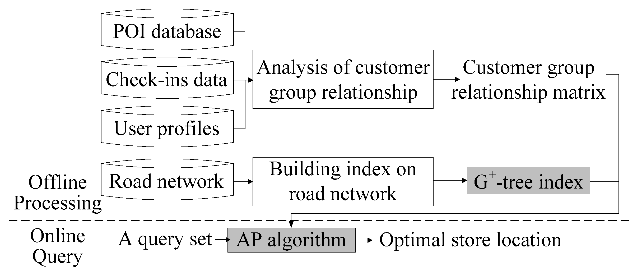
As shown in Figure 2, the system framework used in this study includes two stages: offline processing and online query. Offline processing starts by analyzing the similarities among the customer groups of various POIs to convert them into customer similarity scores. These scores are stored in a matrix to set the influence score of the POIs in the second stage. The G-tree index is then established to swiftly calculate the road distance between two points in the second stage. After the query set Q = {pP, nP, rP} is input by the user, the second stage is initialized to identify the optimal store location for Q.
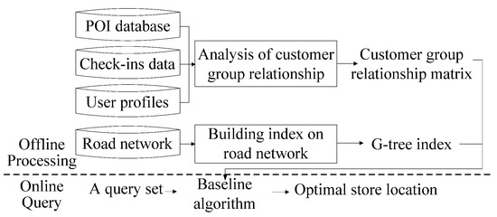
Figure 2.
System framework of the baseline algorithm.
4.2. Analysis of the Similarities among Customer Groups
The analysis of customer groups includes three steps: (1) customer clustering, (2) find the common characteristics of the customers in each group, and (3) calculate the customer similarity scores to store in a matrix.
If user u has checked in at POI p, we can regard u as a customer of p. We can therefore use check-in data to identify the customers of each store and cluster them according to their characteristics using their user profiles. These characteristics allow for us to calculate the similarity scores among the customer groups of different POIs.
4.2.1. Customer Clustering
Before clustering the customers, we first would normalize their user profiles. Suppose that the attributes of user profiles include age, gender, educational background, and annual income. For age and annual income, which are naturally positive, we divide them by the maximum values to normalize them to between 0 and 1. For gender, we set female as 0 and male as 1. Educational background has a sequential order. For such attributes, if there are n options, we can set the value of the ith option as i/(n − 1) to normalize it to between 0 and 1.
Following normalization, we divide the customers into several groups. As we do not know the distributions of the customers of each store, we follow the suggestion of [25] and use the expectation-maximization clustering method. We refer to these groups as customer groups.
4.2.2. Identification of Common Characteristics
If the values of characteristic ai for the customer group are concentrated, then more members of customer group have this characteristic, making ai representative of the customer group as a whole. We adopt the coefficient of variation to assess the degree of dispersion among the values. A smaller coefficient of variation for ai of the customer group means that the characteristic is more representative of the customer group. We rank the coefficient of variation of each characteristic of each customer group in ascending order and use the top n characteristics to represent the customer group. The coefficient of variation is equal to σ/μ, where σ is the standard deviation and μ is the mean.
4.2.3. Calculation of Customer Similarity Scores
In this step, we calculate CS(pi, pj), the customer similarity score between POIs pi and pj. The result is stored in matrix M. We define CS(pi, pj) as the expected number of customers that pi can attract from pj. Suppose that the customer groups of pi and pj can be respectively expressed as {cgi1, cgi2, …, cgik} and {cgj1, cgj2, …, cgjk}. For every cgjn of pj, we first evaluate the similarity between cgjn and all customer groups of pi. Then, we select the highest one among them as the probability that members of cgjn will become customers of pi. The expected number of customers equals the sum of the number of customers multiplied by this probability. Thus, CS(pi, pj) can be calculated as follows:
where |cgjn| is the number of customers in cgjn, and cgSIM(cgjn, cgim) denotes the degree of similarity between customer groups cgjn and cgim.
CS(pi, pj) = ∑n=1~k|cgjn| × maxcgim∈picgSIM(cgjn, cgim),
We next introduce the means of calculating the degrees of similarity between customer groups (i.e., cgSIM(cgjn, cgim) in Equation (3)). This is achieved using a modified form of Jaccard similarity. We use the common characteristic set to represent the customer group and calculate the degree of similarity between two customer groups by calculating the degree of similarity between the two common characteristic sets. Jaccard similarity J(A,B) calculates the degree of similarity between two sets, A and B [26]. The value of J(A,B) ranges from 0 to 1. When A and B are identical, J(A,B) equals 1. When A and B are completely different, J(A,B) equals 0. J(A,B) therefore equals the intersection of A and B divided by the union of A and B. However, Jaccard similarity only considers the intersection and union of two sets and does not consider the distributions of common characteristics. We thus propose modifying the Jaccard similarity by replacing the number of intersections of two common characteristic sets with the total similarity between the shared distributions of common characteristics. The similarity cgSIM(cgi, cgj) between two customer groups cgi and cgj can then be calculated as follows:
where D(cg, f) denotes the distributions of customers in customer group cg with regard to common characteristic f, and fSIM(∙,∙) is the similarity between the distributions of common characteristics.
We calculate the degrees of similarity between two distributions of common characteristics (i.e., fSIM(∙,∙) in Equation (4)) using a modified form of Jensen-Shannon (JS) divergence. JS divergence [27] is a modified form of Kullback-Leibler (KL) divergence. KL divergence KLD(Da|Db) measures the differences between two distributions, Da and Db, as follows:
However, KL divergence measures non-symmetric difference, which means that KLD(Da|Db) does not equal KLD(Db|Da). To solve this problem, JS divergence (which is symmetric) is calculated as follows:
where Dm = (Da + Db)/2. The value of JSD(Da|Db) ranges from 0 to 1. The value of JSD(Da|Db) is proportional to the difference between distributions Da and Db. JSD(Da|Db) equals 0 at the minimum difference between Da and Db and 1 at the maximum difference between Da and Db. As similarity is the opposite of difference, we can design a formula to represent the similarity between two distributions of common characteristics as follows:
fSIM(Da, Db) = 1 − JSD(Da, Db).
4.3. Establishment of Roadmap Index
We used the G-tree index to help the system swiftly calculate the road distance between points. G-tree is an efficient tree index proposed by Zhong et al. [28] for KNN searches on road networks. They recursively partition the road network into sub-networks and build a tree structure on top of subnetworks where each G-tree node corresponds to a sub-network. Due to length limitations, please refer to [28] for further details on G-tree.
4.4. Online Query Process of Baseline Algorithm
In the online query stage, the query user q provides a query set (pP, nP, rP), where pP is a set of PPOIs, nP is a set of NPOIs, and rP is a set of RPOIs. The system uses the following algorithm to find an optimal store location for q.
The optimal solution may be any point on any edge in the roadmap, representing an infinite solution set. Below we present a theorem that the lowest location score on edge e will appear at specific points. Thus, we need only calculate the location scores of these specific points to find the optimal solution.
Theorem 1.
The lowest location score on edge e must be at the break point or vertex of e.
Proof.
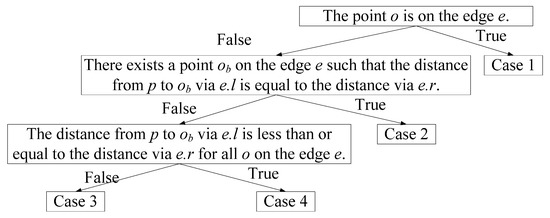
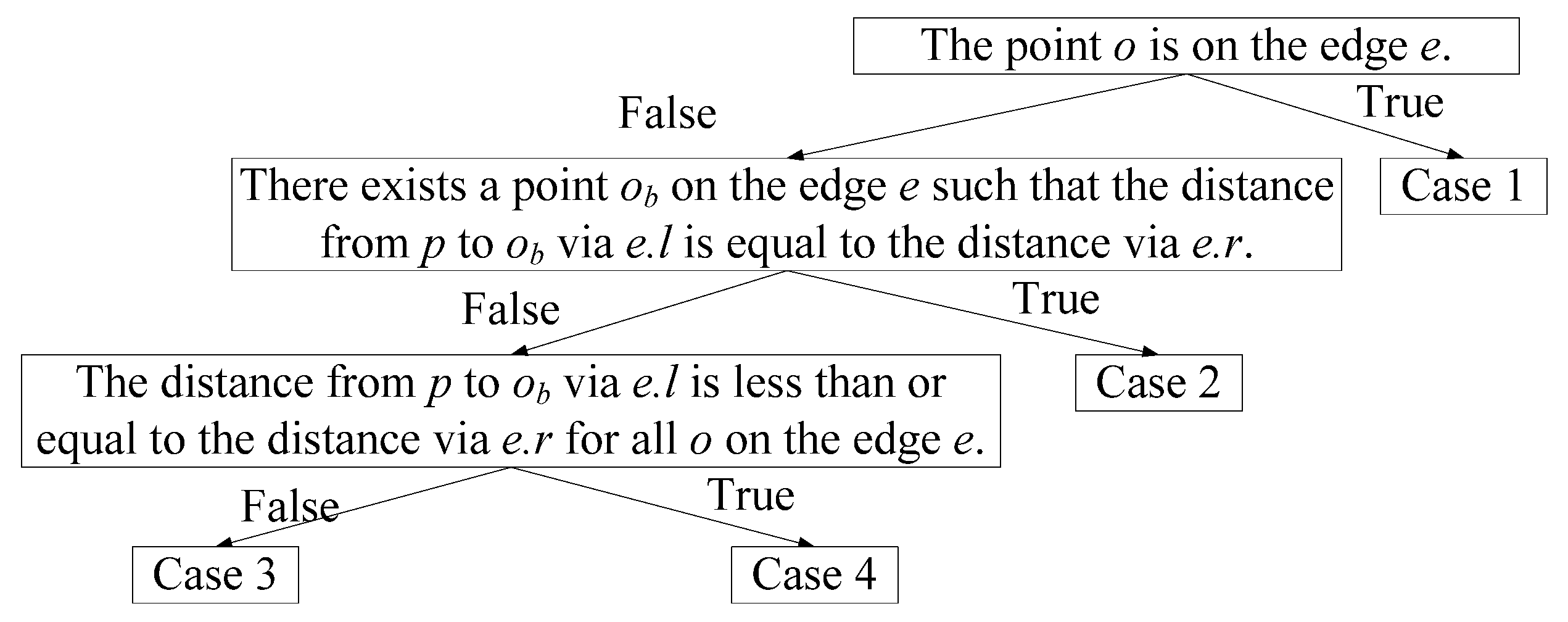
Consider POI p and point o, which is any given point on edge e. The shortest distance between p and o, dist(p, o), can be one of four cases depending on three conditions, as shown in Figure 3: (1) Is o on e? (2) Is e at a certain point ob so that the path length from p to ob via e.l equals the path length from p to ob via e.r (i.e., ∃o∈e, dist(p,e.l) + dist(e.l,o) = dist(p,e.r) + dist(e.r,o))? (3) Do all points o on e cause the path length from p to o via e.l to be less than or equal to the path length from p to o via e.r (i.e., ∀o∈e, dist(p,e.l) + dist(e.l,o) ≤ dist(p,e.r) + dist(e.r,o))?

Figure 3.
Decision tree for dist(p, o).
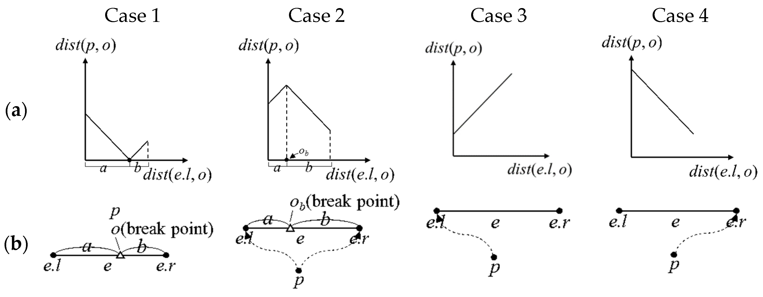
The graphs of dist(p,o) for each of these cases are as shown in Figure 4a, where the x axis represents the shortest distance dist(e.l,o) from the left vertex of e to o, and the y axis represents dist(p,o). The corresponding road diagrams are displayed in Figure 4b, where the dotted line is the shortest path from p to o. When o is on e, dist(p,o) represents Case 1, which is a piecewise linear function where dist(p,o) equals 0 when o is p. We refer to o as being p on a break point on e. When o is not on e, dist(p,o) = min(dist(p,e.l) + dist(e.l,o), dist(p,e.r) + dist(e.r,o)), and the possible conditions are Cases 2, 3, and 4. If a certain point ob can be found on e so that dist(p,e.l) + dist(e.l,ob) = dist(p,e.r) + dist(e.r,ob), dist(p,o) represents Case 2, which is a piecewise linear function. We refer to ob as being p on a break point on e. If a certain point o can be found on e, dist(p,e.l) + dist(e.l,o) ≤ dist(p,e.r) + dist(e.r,o), dist(p,o) represents Case 3, which is a linear function. Otherwise, dist(p,o) represents Case 4, which is also a linear function. Thus, dist(p,o) is either a linear function or a piecewise linear function.
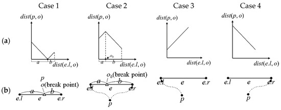
Figure 4.
Four cases of dist(p,o): (a) graphs of dist(p,o); (b) corresponding road diagrams.
CI(Q, p) is the influence score of p. For identical query sets, CI(Q, p) is constant. dist(p,o) × CI(Q, p) can be regarded as a linear function or a piecewise linear function multiplied by a constant, which results in a linear function or piecewise linear function.
Based on Equation (2), LS(o, pP, nP) = ∑p∈pP∪nP dist(o,p) × CI(Q, p). The location score is the sum of multiple linear functions or piecewise linear functions. Thus, the form of the location score is a piecewise linear function.
Consider linear function f and closed interval [a,b], where x is any point in (a,b). f(a) must be less than or equal to f(x), or f(b) must be less than or equal to f(x), as f is linear. A piecewise linear function comprises several linear functions. If we can segment a piecewise linear function into several linear functions in different closed intervals, then the minimum value of the piecewise linear function must be located at the ends of these intervals.
Suppose |pP∪nP| is n1, and the break points of pP∪nP on e are {o1, o2, …, on2}. If i > j, then dist(oi, e.l) ≥ dist(oj, e.l). Furthermore, n2 ≤ n1 because each POI on e has only 0 or 1 break points. The form of the location score is a piecewise linear function. We can segment the location score into several linear functions in different closed intervals, and the ends of these intervals are {e.l, o1, o2, …, on2, e.r}. Thus, the point with the lowest location score on e must be at the break points or vertex of e. Q.E.D.
Using Theorem 1, we only need to calculate the location scores of the break points and vertices of all the edges to obtain the optimal solution. The complete process of the baseline algorithm is as follows:
- Step 1.
- For each POI pj, use Equation (1) and the customer similarity score matrix calculated offline to evaluate its influence score CI(Q, pj), where Q is given by the query user and is equal to {pP, nP, rP}.
- Step 2.
- Find the break points and vertices of all edges.
- Step 3.
- Calculate the location scores of all the break points and vertices of all edges and select the optimal solution.
An example of the baseline algorithm is presented in Appendix A. □
5. Area-Pruning Algorithm
This Section introduces the area-pruning (AP) algorithm, which is more efficient than the baseline algorithm. We first analyze the shortcomings of the baseline algorithm and introduce suggested changes to the system framework. We then propose a novel road index, the G+-tree index. This is used to present the procedure of the AP algorithm and an example application.
5.1. Shortcomings of Baseline Algorithm
While the baseline algorithm is intuitive, it requires calculating the location scores of all of the break points and vertices on all edges. However, a real-world roadmap often contains tens of thousands of edges, and the number of POIs provided by the query user is generally several hundred. We therefore proposed, first, pruning areas that cannot hold the optimal location to enhance the efficiency of the algorithm.
5.2. System Framework with AP Algorithm
To swiftly derive the upper and lower bounds of the road distance between POI p and any given point within a G-tree node, we stored extra information in the nodes to create a G+-tree. The bounds of the location scores are used to determine whether the optimal store location may exist within the G+-tree node. If not, we skip the road sections in this G+-tree node, thereby accelerating the speed of the query algorithm. These modifications are depicted in Figure 5.

Figure 5.
System framework of the AP algorithm.
5.3. G+-Tree Index
The G+-tree index was modified from G-tree. In addition to the original G-tree information, we calculate three values for each G+-tree node Gx based on the borders of Gx, namely, low(Gx), high(Gx), and maxEdge(Gx), and store these values. Below we introduce the definition of a border and the calculations for these three values.
Definition of Borders: Given subgraph Gx = (Vx, Ex) of G = (V, E), vertex u ∈ Vx is called a border if ∃(u,v) ∈ E and v ∉ Vx.
Border low(Gx): This is used to underestimate the road distance from any border of Gx to any point v within Gx. If Gx is a leaf node, then low(Gx) is the road distance from any border of the smallest Gx to any point v within Gx. If Gx is not a leaf node, then low(Gx) is the road distance from the border of the smallest Gx to the border of subnode Gx+1 plus low(Gx+1). The calculation method is as follows:
Border high(Gx): This is used to overestimate the road distance from any border of Gx to any point v within Gx. If Gx is a leaf node, then high(Gx) is the road distance from any border of the largest Gx to any point v within Gx. If Gx is not a leaf node, then high(Gx) is the road distance from the border of the largest Gx to the border of subnode Gx+1 plus high(Gx+1). The calculation method is as follows:
Border maxEdge(Gx): This is the length of the longest edge in Gx. If the left vertex e.vl belongs to Gi, then we say that e belongs to Gx. The calculation method is as follows:
MaxEdge(Gx) = maxe∈Gxe.length.
5.4. Online Process of AP Algorithm
The AP algorithm avoids unnecessary G+-tree nodes to enhance efficiency. We derived a theorem to help us determine what the best possible score may be in the G+-tree node Gi. If this score is poorer than the current best location score, then we can skip Gi. The theorem utilizes a lower bound LB(Gi, p), which we define as follows:
Consider o as any given point on any given edge in Gi. For POI p, we define the lower bound LB(Gi, p) of a CI(Q, p) × dist(o,p). If the influence score of p is a positive number, then LB(Gi, p) equals the influence score multiplied by an underestimated dist(o,p). If the influence score of p is a negative number, then LB(Gi, p) equals the influence score multiplied by an overestimated dist(o,p). The calculation method is as follows:
where lowDist(Gi,p) is a non-negative number less than or equal to the distance from p to any given vertex in Gi, highDist(Gi,p) is a non-negative number greater than or equal to the distance from p to any given vertex in Gi, and maxEdge(Gi) is the length of the longest edge in Gi.
Theorem 2.
Consider the query set (pP, nP, rP), where p is a POI in pP and nP. Location o is any given point on any given edge in Gi. The best location score in Gi must be greater than or equal to the sum of all LB(Gi, p):
Proof.
Please see Appendix B. □
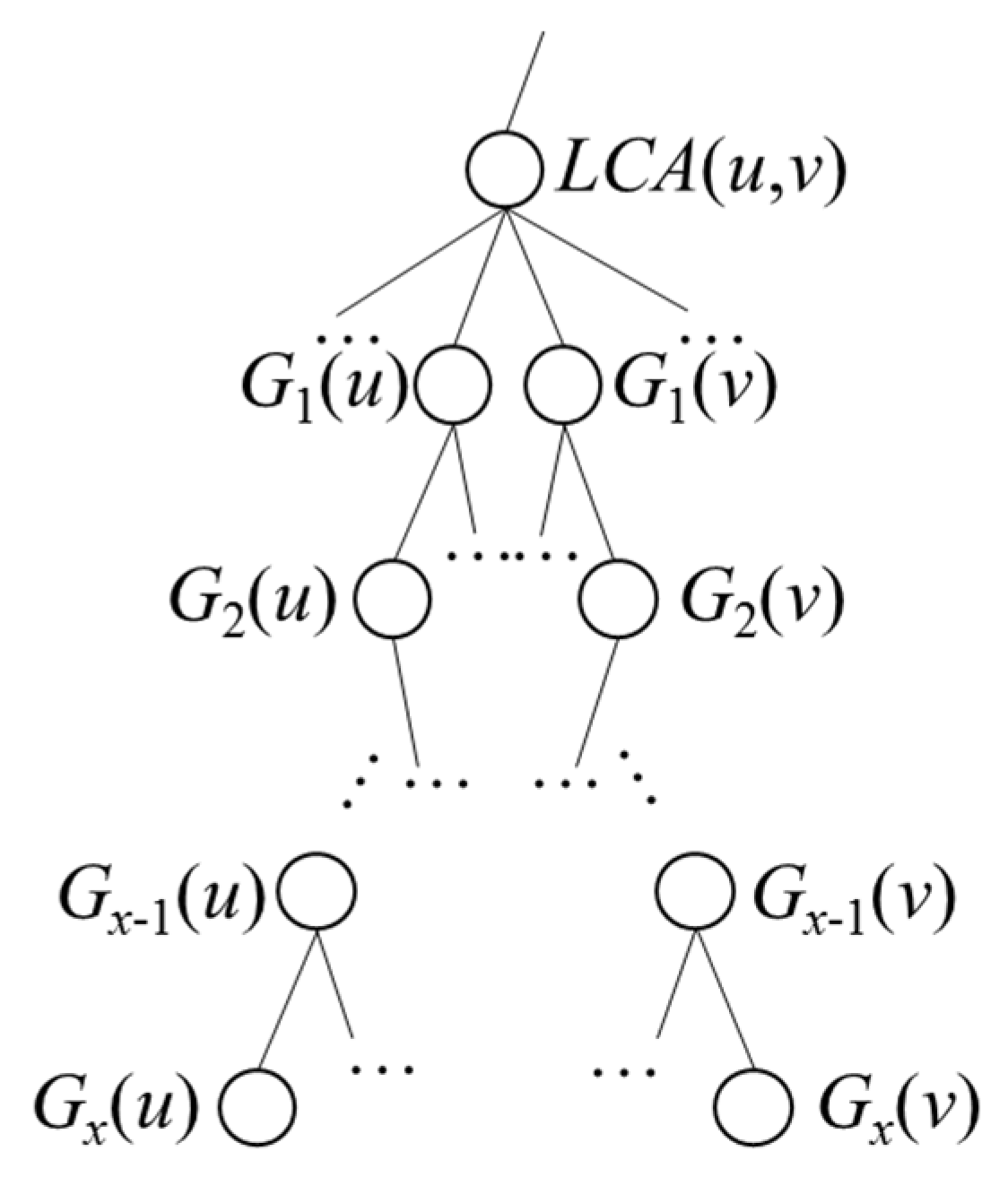
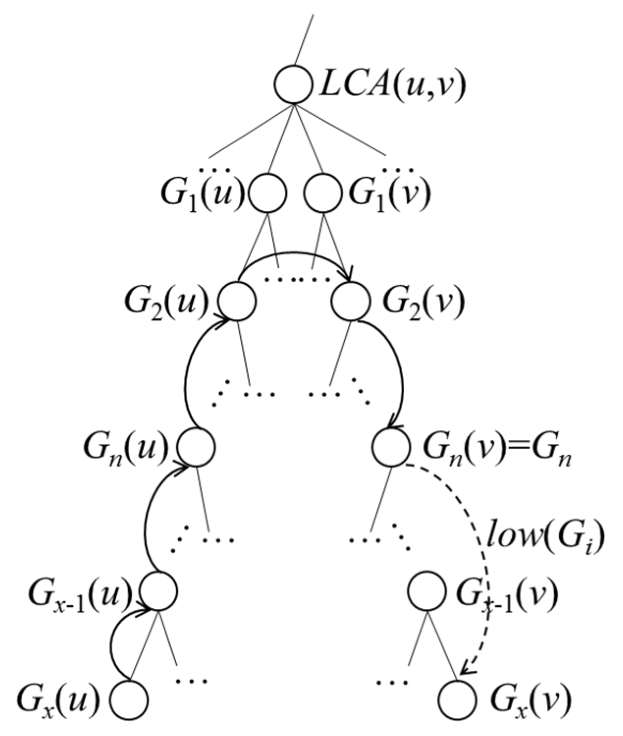
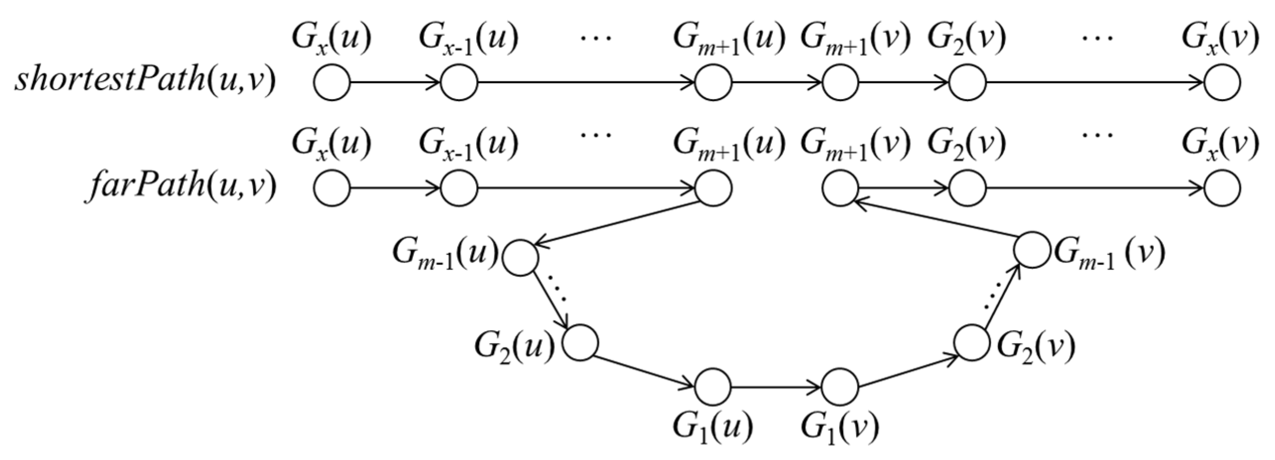
Theorem 2 makes use of lowDist(Gi,p) and highDist(Gi,p). We use G+-tree and low(Gi) and high(Gi) to calculate lowDist(Gi,p) and highDist(Gi,p). Below, we introduce relevant symbols and calculation methods. Suppose we want to calculate dist(u,v), the road distance from u to v. leaf(u) and leaf(v) are the G+-tree nodes for u and v. As indicated by [28], if u and v do not belong to the same G+-tree leaf node, then any path from u to v must pass through a series of G+-tree nodes Gx(u), Gx−1(u), …, G1(u), G1(v), G2(v), …, Gx(v), as shown in Figure 6, where Gx(u) = leaf(u), Gx(v) = leaf(v), and LCA(u,v) are the lowest common ancestors of Gx(u) and Gx(v).

Figure 6.
G+-tree nodes passed through from u to v.
If u belongs to Gi, then lowDist(Gi, u) equals 0. If not, then, as shown in Figure 7, we let Gi equal Gn(v), such that lowDist(Gi, u) is the distance traveled from u to Gx(u), Gx−1(u), …, G1(u), G1(v), G2(v), …, Gn(v) plus low(Gi).

Figure 7.
Case 2 of lowDist(Gi, u).
Theorem 3.
lowDist(Gi, u) must be a non-negative number less than or equal to the distance from u to any given vertex in Gi.
Proof.
Please see Appendix C. □
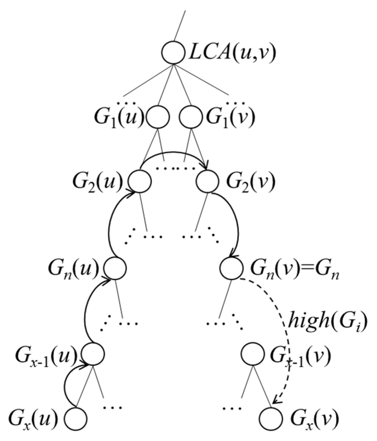
If u belongs to Gi, as shown in Figure 8, we let Gi equal Gn(v), such that highDist (Gi, u) is the distance traveled from u to Gx(u), Gx−1(u), …, G1(u), G1(v), G2(v), …, Gn(v) plus high(Gi). Otherwise, as shown in Figure 9, highDist (Gi, u) is the distance traveled from u to Gx(u), Gx−1(u), …, G1(u), Gi plus high(Gi).

Figure 8.
Case 1 of highDist(Gi, u).
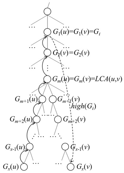
Figure 9.
Case 2 of highDist(Gi, u).
Theorem 4.
highDist(Gi, u) must be a non-negative number greater than or equal to the distance from u to any given vertex in Gi.
Proof.
Please see Appendix D. □
As with the application of G-tree to calculate the road distance between two points, we can utilize a dynamic programming algorithm to calculate lowDist(Gi, p) and highDist(Gi, p). The low(Gi) and high(Gi) involved in the calculations are derived offline. We can then use lowDist(Gi, p) and highDist(Gi, p) to calculate LB(Gi, p).
Pseudocode for the AP algorithm is shown in Algorithm 1, where the query user inputs query set Q = {pP, nP, rP}.
| Algorithm 1: Area-Pruning algorithm | |
| Input: POI database, customer similarity score matrix Output: Optimal location | |
| 1 | for each p in POI dataset |
| 2 | p.w←set_impact(p, customer similarity score matrix) |
| 3 | end for |
| 4 | for each node Gi in traverse G+-tree |
| 5 | if Theorem 2 is satisfied |
| 6 | pruning(Gi) |
| 7 | end if |
| 8 | if is_leaf_node(Gi) |
| 9 | break points, vertexes←find(Gi) |
| 10 | location scores←calculate_scores(break points, vertexes) |
| 11 | optimal solution←update(location scores) |
| 12 | end if |
| 13 | end for |
| 14 | return optimal solution |
- Step 1.
- For each POI p, use Equation (1) and the customer similarity score matrix calculated offline to evaluate its influence score CI(Q, p). (lines 1–3)
- Step 2.
- Visit the G+-tree of the roadmap, and retrieve the next tree node Gi. (line 4)
- Step 3.
- If the current best location score ≤ ∑p∈pP∪npLB(Gi, p), then, according to Theorem 2, we can prune Gi and return to Step 2. Otherwise, move to Step 4. (lines 5–7)
- Step 4.
- Check if Gi is a leaf node. If it is a non-leaf node, then return to Step 2. Otherwise, find the break points and vertices of all edges in Gi, calculate the location scores of these points, and update the current best solution. (lines 8–12)
- Step 5.
- If the entire G+-tree has been visited, then return the optimal solution. (lines 13–14)
An example of the AP algorithm is presented in Appendix E.
6. Area-and-Edge-Pruning Algorithm
The area-and-edge-pruning (AEP) algorithm modified Step 2.3 (as shown in Figure 5) of AP. In the following, we first analyze the shortcomings of the AP algorithm, then go on to present an overview of the AEP algorithm.
6.1. Shortcomings of AP Algorithm
The AP algorithm avoids unnecessary G+-tree nodes and thereby enhances computational efficiency. However, when G+-tree leaf node Gl is not pruned, the location scores of all the break points and vertices of edges in Gl must still be calculated. We therefore developed an edge-pruning method that avoids calculating the location scores of unnecessary break points on edges to further increase computational efficiency.
6.2. Online Process of AEP Algorithm
When the AP algorithm cannot prune G+-tree node Gi, the AEP algorithm determines whether some of the edges in Gi can be pruned. We derived a theorem to help us determine whether a better solution exists on the break points of an edge to avoid calculating the location scores of unnecessary break points.
Theorem 5.
Consider edge e and query set (pP, nP, rP). We refer to nP∪rP as POIs. We use BP(p,e) to represent a break point of POI p on e and use BPs(POIs,e) to represent a set of all p on e in the POIs. Thus, we have the following:
where the former term is the best location score on e; the latter can be regarded as the lower bound of this location score.
Proof.
Please see Appendix F. □
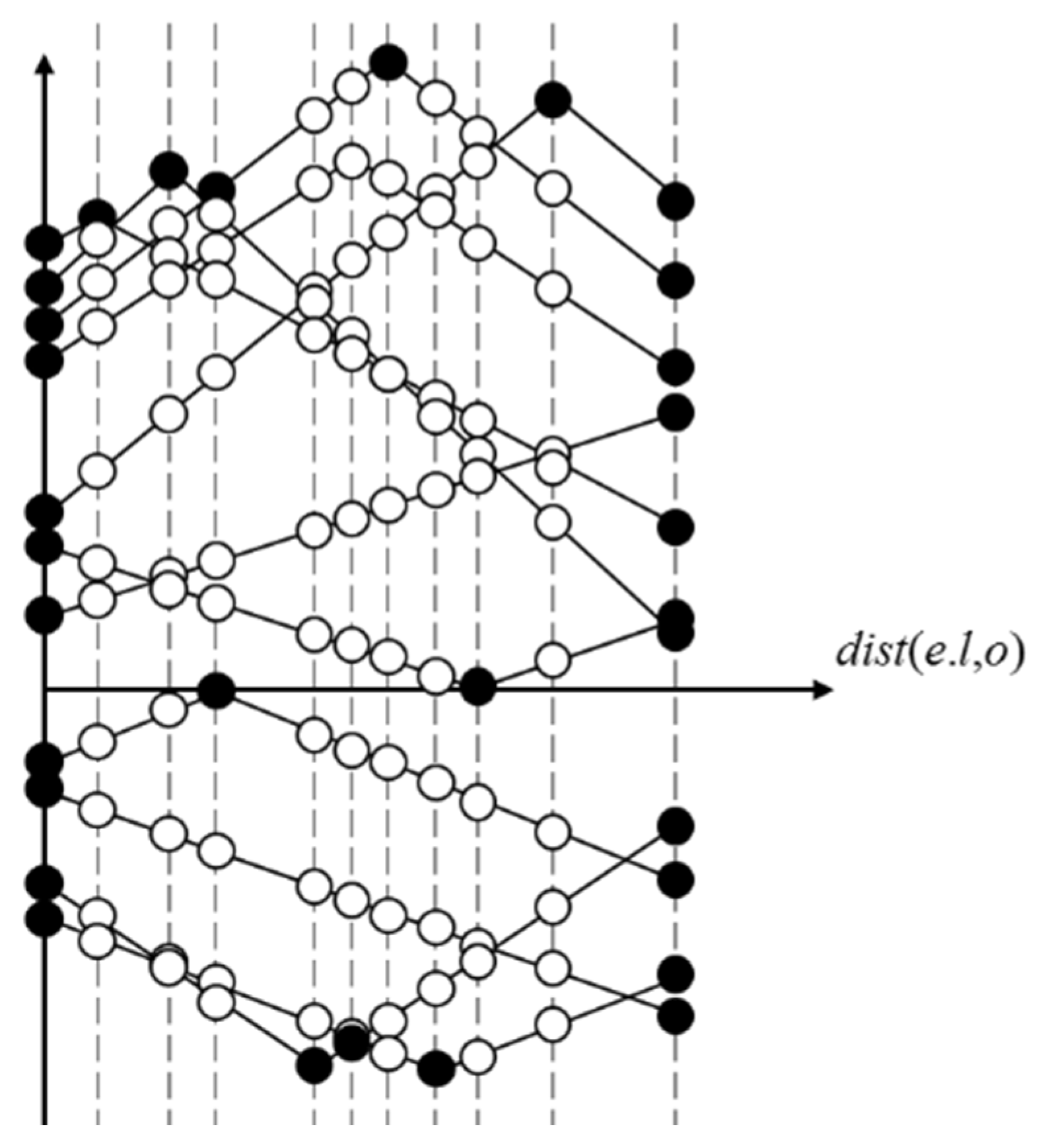
According to Theorem 5, we need only calculate the dist(o,p) × CI(Q, p) of two vertices and the break point from each p to e to determine whether this edge can be pruned. Take dist(o,p) × CI(Q, p) on an edge e as an example, as shown in Figure 10. We need only calculate the black points: if e can be pruned, then the white points do not need to be calculated.

Figure 10.
Example of dist(o,p) × CI(Q, p) on e.
For query set Q = {pP, nP, rP}, the procedure of the AEP algorithm is as follows:
- Step 1.
- For each POI p, use Equation (1) and the customer similarity score matrix calculated offline to evaluate its influence score CI(Q, p).
- Step 2.
- Visit the G+-tree of the roadmap and retrieve the next tree node Gi.
- Step 3.
- If the current best location score ≤∑p∈pP∪npLB(Gi, p), then, according to Theorem 2, we can prune Gi and return to Step 2. Otherwise, move to Step 4.
- Step 4.
- Check if Gi is a leaf node. If it is a non-leaf node, then return to Step 2. Otherwise, go to Step 5.
- Step 5.
- Retrieve the next edge ej in Gi.
- Step 6.
- If the current best location score ≤ , then, according to Theorem 5, prune ej. Otherwise, go to Step 7.
- Step 7.
- Find the next break point or vertex on ej, calculate the location scores of this point, and update the current best solution.
- Step 8.
- If all break points and vertices in ej have been considered, then return to Step 5.
- Step 9.
- If the entire G+-tree has been visited, then output the optimal solution.
An example of the AEP algorithm is presented in Appendix G.
7. Experiments
The system framework in this paper comprises two stages: offline processing and online query. We conducted a series of experiments to assess the effectiveness of the customer similarity scores in offline processing and the efficiency of the online query. Finally, we conducted a case study using real-world data from a fast-food restaurant to verify the applicability of the proposed system.
7.1. Parameter Settings
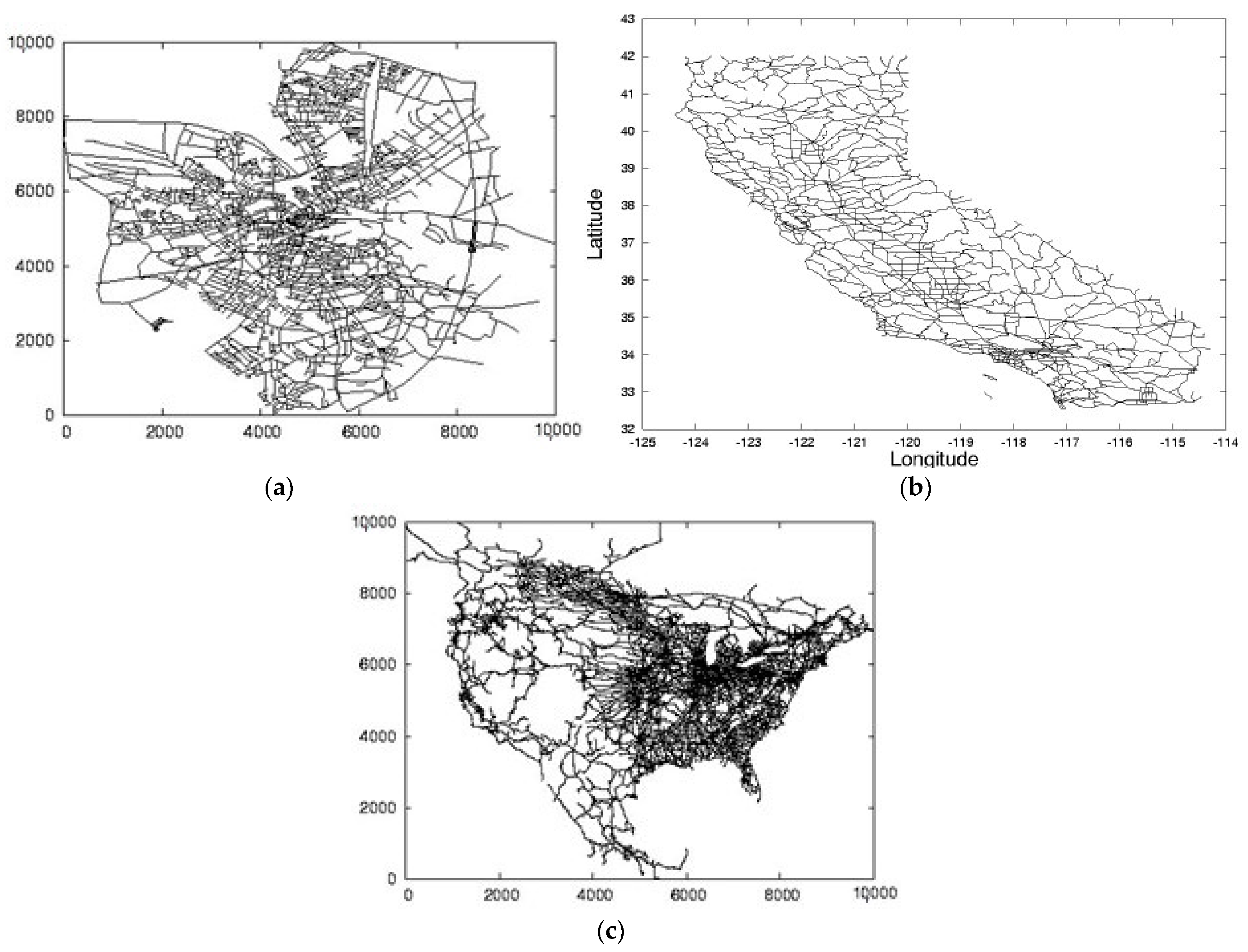
The data used in the experiments included roadmaps, POI databases, user profiles, and check-in data. For the roadmaps, we employed three real-world datasets provided by [29], which are displayed in Figure 11. From the smallest to the largest in size, the three datasets were retrieved from Oldenburg (OL), California (CAL), and North America (NA). The OL dataset contains 6105 nodes and 7035 edges. The CAL dataset has 21,048 nodes and 21,693 edges. The NA dataset includes 175,813 nodes and 179,178 edges.

Figure 11.
Roadmap datasets: (a) Oldenburg, (b) California, (c) North America.
As there were no POI databases, user profiles, and check-in data corresponding to the three roadmaps, we generated synthetic datasets as follows. First, 10% of the points in the roadmaps were randomly selected as POIs. Next, αk customer groups were generated for each POI, each group containing the same number of people. Each customer group had 10 characteristics, and αn of them were randomly selected as common characteristics. We let the values for these follow a Gaussian distribution without loss of generality. We assumed the values of the other characteristics were evenly distributed. To generate users, we marked a customer group for each user to serve as a standard solution for clustering.
The experiments were implemented in Java running Ubuntu 16.04 64 bits OS at Intel Core i5-6400 clock of 2.7 GHz with 4 cores and a memory of 16 GB. Each experiment was conducted 30 times, and the results were averaged. Table 3 lists the parameter settings used in experiments, with bold font indicating default settings. As this paper represents the first attempt to use LBSN datasets to calculate the influence of POIs on the customer group of a new store, we were unable to conduct a performance comparison with similar algorithms. The AEP, the second algorithm designed to reduce computational load, takes 20 s at most, and on average less than 5 s regardless of the map and query condition. These results are well within expected standards and verify that the algorithm achieves its intended purpose.

Table 3.
Summary of experiment parameters.
7.2. Experiments Regarding Offline Processing
In this section, we demonstrate the effectiveness of the customer similarity score. We (1) compare the accuracy of clustering methods and (2) discuss means of observing the clustering results of different simulation data to identify suitable parameter settings (k and n). We show that when k = αk and n = αn, two stores with a greater degree of similarity between their customer groups will have a higher customer similarity score, verifying the validity of the concept.
7.2.1. Comparison of Clustering Method Accuracy
We compared one of the most well-known clustering methods, k-means, with the expectation-maximization (EM) algorithm described in Section 4. The customers of a POI p were divided into several customer groups cgi. The clustering accuracy with regard to p was defined as the number of correctly-clustered customers divided by the number of customers that p has. The mean clustering accuracy was defined as the mean clustering accuracy rate for all POIs.
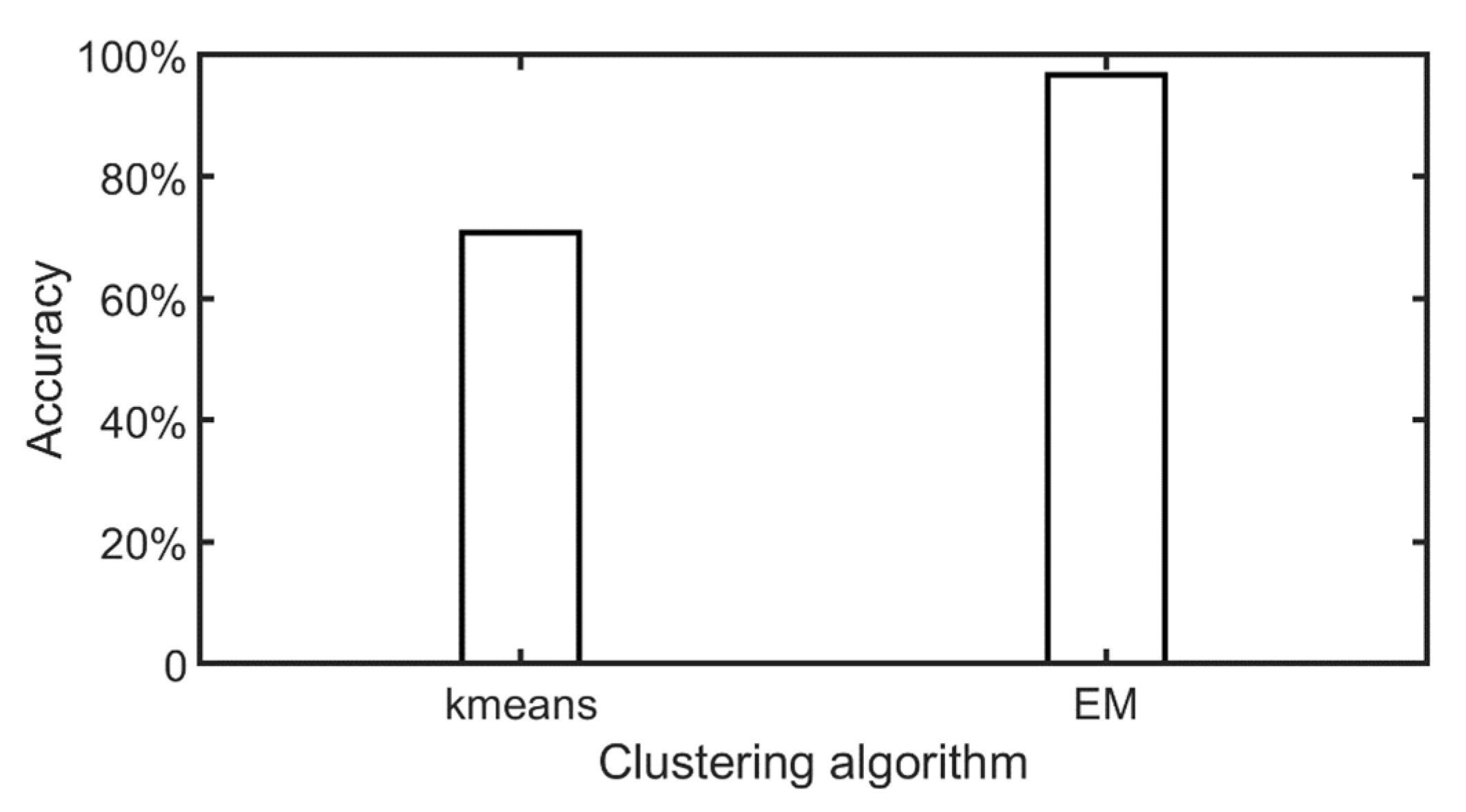
We generated synthetic data for the POI databases, user profiles, and check-in data. For the sake of convenience, we selected the smaller OL dataset for this experiment. Default values were adopted for the remaining parameters (k and n); that is, each POI had four customer groups, each with four common characteristics. The customers of each POI were divided into four customer groups using the k-means and EM clustering methods. As shown in Figure 12, the mean clustering accuracy of k-means was 70.83%, and that of the EM clustering methods was 96.73%. We therefore adopted the EM clustering methods in subsequent experiments.
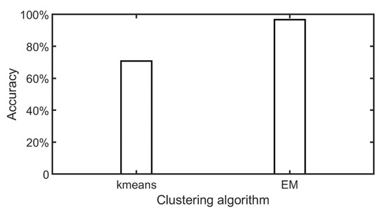
Figure 12.
Clustering accuracy of different clustering methods.
7.2.2. Setting Suitable Numbers of Customer Groups and Characteristics
In this section, we discuss the means of identifying suitable settings for parameters k and n. With suitable parameters, a well-designed customer similarity score will produce a higher score when a greater degree of similarity exists between the customer groups of two stores. We randomly divided the customers of store p into two groups and set them as the customers of two simulated stores p1 and p2. As they were customers of the same store, the customer similarity scores of p1 and p2 should be as high as possible. The highest possible score for CS(p1, p2) is the number of customers that p2 has, and the highest possible score for CS(p2, p1) is the number of customers that p1 has. We therefore set an evaluation score evalNS(p) as (CS(p1, p2) + CS(p2, p1))/the number of customers that p1 has plus the number of customers that p2 has.
AvgEvalNS is the average of the evalNS(p) of all POI p in the roadmap. A higher AvgEvalNS means that the parameter settings (k and n) for the customer similarity score are more suitable.
When generating synthetic data for the POI databases, user profiles, and check-in data, we selected the smaller OL dataset for the sake of convenience. Default values were adopted for the remaining parameters (k, n, and clustering method); that is, each POI had four customer groups, each with four common characteristics, clustered by EM.
The AvgEvalNS resulting from different parameter settings (k and n) are presented in Figure 13. In Figure 13a, AvgEvalNS gradually rises when k = 4, 5, 6 and n ≤ 4 but declines sharply when n > 4. This is because adopting more than x characteristics to calculate the customer similarity score when a customer group has only x common characteristics will cause irrelevant characteristics to be included in the calculations, resulting in poor AvgEvalNS values. If fewer than x characteristics are used, all included characteristics are relevant, so the values of AvgEvalNS will be constant. With k = 2, 3, the values of AvgEvalNS do not present the above trend because the setting for k is too low, which causes clustering errors and thus poor AvgEvalNS values. Thus, the optimal setting for k is 4.

Figure 13.
AvgEvalNS with (αk = 4, αn = 4) resulting from different k, n. (a) resulting from different n. (b) resulting from different k.
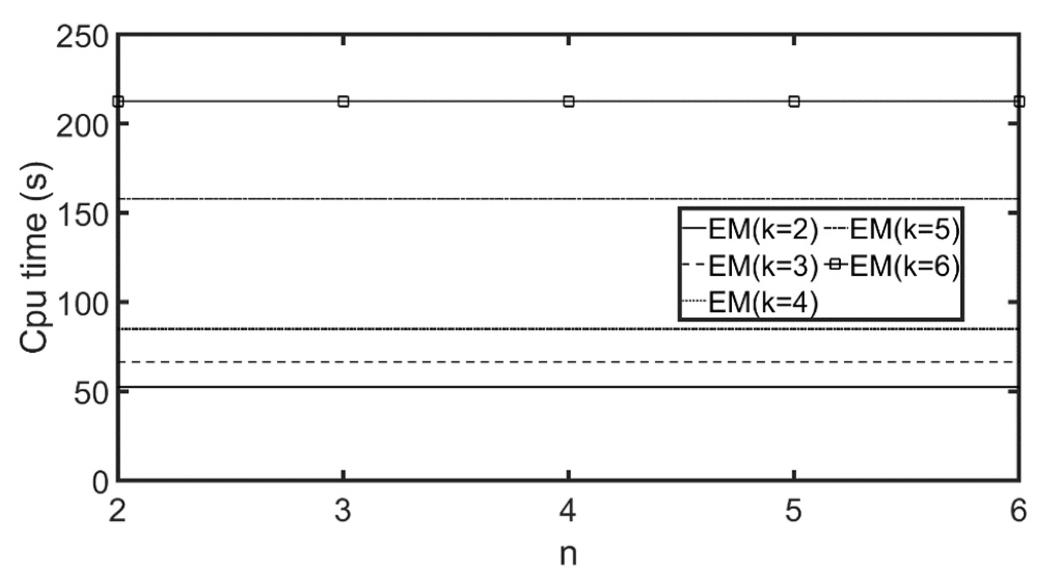
In Figure 13b, when k ≤ 4, the values of AvgEvalNS show a steeply-increasing trend. When c > 4, the values of AvgEvalNS remain constant. This is because dividing the customers of a POI into fewer than y customer groups will cause many customers that should not belong to the same group to be grouped together. More clustering errors will reduce the value of AvgEvalNS. If we divide the customers into more than y customer groups, it will cause some customer groups to be divided into smaller subgroups; nevertheless, these clustering results are not incorrect, so the AvgEvalNS value will not differ greatly. Thus, setting k at 4, 5, or 6 is acceptable. However, since a greater k value will increase computation costs (as shown in Figure 14), the optimal setting for k is 4.

Figure 14.
Computation time for customer similarity scores with different k, n (αk = 4, αn = 4).
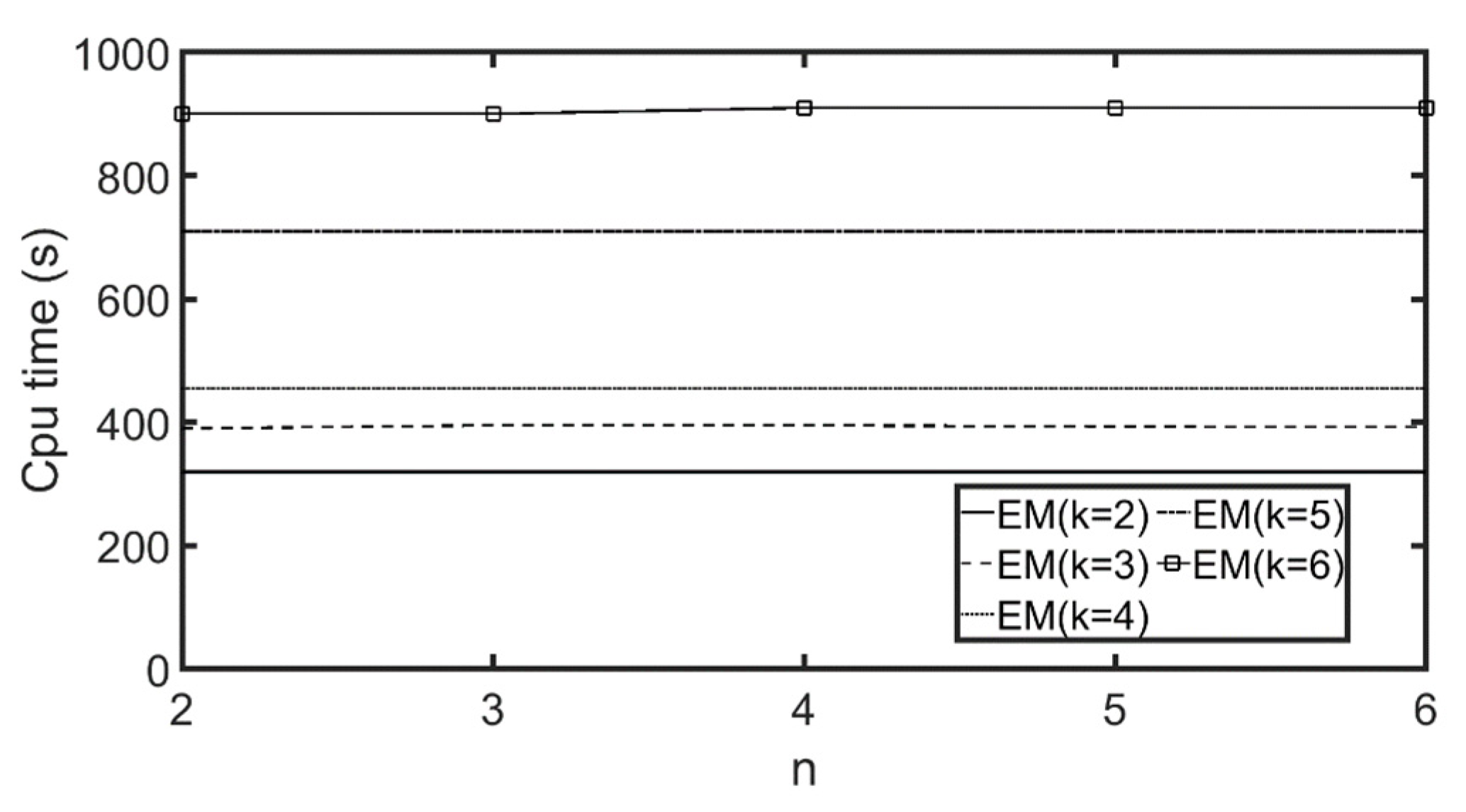
We then used the CAL and NA roadmaps, which were larger than the OL roadmap. Figure 15 and Figure 16 display the results for the CAL roadmap, and Figure 17 and Figure 18 show the results for the NA roadmap. Again, similar trends were achieved. Computation time with different k and n ranged from 52 s to 215 s for the OL roadmap, from 330 s to 916 s for the CAL roadmap, and from 1163 s to 5949 s for the NA roadmap. Larger roadmaps take longer to compute because they contain more POIs, and, therefore, it takes longer to calculate the customer similarity scores.

Figure 15.
AvgEvalNS with (αk = 4, αn = 4, CAL) resulting from different k, n. (a) resulting from different n. (b) resulting from different k.
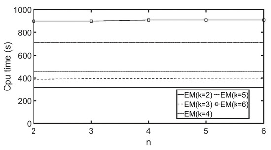
Figure 16.
Computation time for customer similarity scores with (αk = 4, αn = 4, CAL).

Figure 17.
AvgEvalNS with (αk = 4, αn = 4, NA) resulting from different k, n. (a) resulting from different n. (b) resulting from different k.
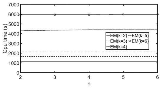
Figure 18.
Computation time for customer similarity scores with (αk = 4, αn = 4, NA).
7.3. Experiments Regarding Online Query
In this Section, we examine the influence of three experiment parameters (namely, poiNum, poiCentralDegree(poiCent), and pRatio) on the computation time exhibited by the different algorithms.
7.3.1. Influence of Changes in poiNum
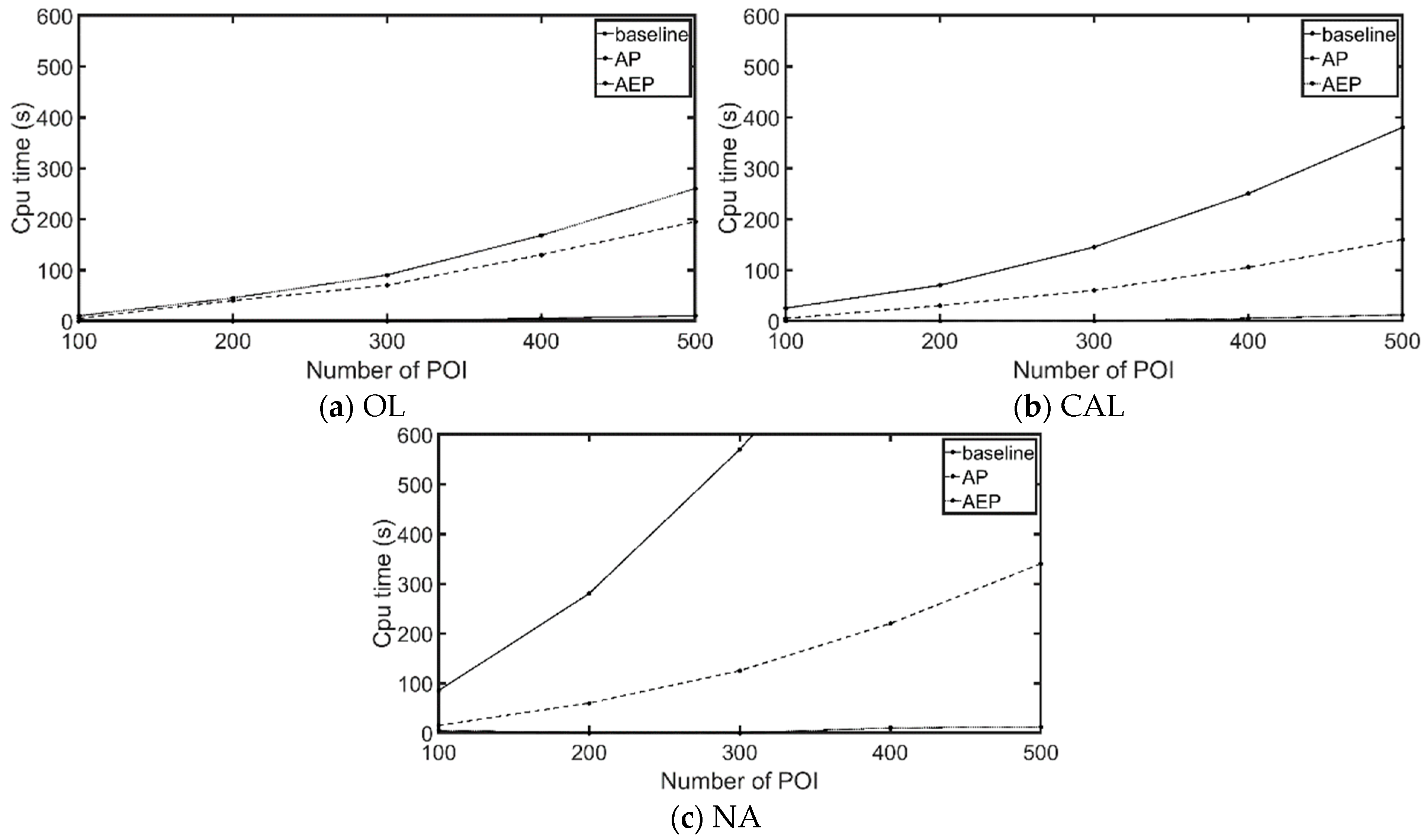
Figure 19 presents the analysis results for the OL, CAL, and NA roadmaps. We set poiNum at 200, 400, 600, 800, and 1000. However, since the OL roadmap only contains 610 POIs, we set poiNum at 100, 200, 300, 400, and 500 for this roadmap. We examined the influence of changes in poiNum on computation time. As shown in Figure 19, as the total number of PPOIs and NPOIs gradually increased, the running time of the baseline rose exponentially. This is because higher numbers of PPOIs and NPOIs mean more possible break points on each edge, thereby greatly increasing the amount of computation. The AP algorithm can prune areas that cannot hold solutions, which reduces the amount of computation. Thus, the running time of the AP algorithm increased more slowly than that of the baseline algorithm. The AEP algorithm further prunes edges that cannot contain solutions. Therefore, although higher numbers of PPOIs and NPOIs mean more possible break points on each edge, the AEP algorithm can thus reduce computation even more with each pruning. As a result, the running time of the AEP algorithm only increased slightly. In all three roadmaps, the experiment results presented the same trends, other than increases in computation time associated with the scope of the roadmap. We therefore only used the largest NA roadmap in the remaining experiments.

Figure 19.
Computation time for queries with different poiNum. (a) OL, (b) CAL, (c) NA.
7.3.2. Influence of Changes in pRatio
Within the context of the considered problem, it is likely that the number of PPOIs would be greater than that of NPOIs. Many NPOIs and more NPOIs than PPOIs would indicate that this area is not a suitable choice for a new store. We therefore set pRatio at 60%, 70%, 80%, 90%, and 100%.
The results of computation time for varying pRatios are presented in Figure 20. The pRatio did not impact the computation time required by the baseline algorithm. This is because the same number of PPOIs and NPOIs results in the same amount of computation in the baseline algorithm. The greater the difference between the scores of the worst solution and the optimal solution, the more obvious the trends of the location of the optimal solution. We found that when the pRatio equals 100%, the difference between the scores of the worst solution and the best solution was 4.95 times that of the difference when the pRatio equaled 60%. As shown in Figure 20, the computation time of the AP algorithm decreased as the proportion of PPOIs increased. This is because more PPOIs mean that the trends of the location of the optimal solution are more obvious and that areas that do not contain the optimal solution are more likely to be pruned. Similarly, the computation time of the AEP algorithm also decreased as the proportion of PPOIs increased. However, as the AEP algorithm prunes edges rather than areas, and as smaller pruning units cause more precise bound estimates, more calculations for unlikely solutions can be reduced. Overall, the computation time was short for all inputs.
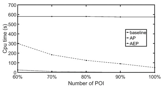
Figure 20.
Computation time for queries with different pRatios.
7.3.3. Influence of Changes in poiCent
This experiment investigated the influence of the degree of concentration among the POIs on computation time. We defined the degree of concentration i as the level of G+-tree nodes that all POIs belong to. A greater i value means that the POIs are more concentrated. Figure 21 shows the results. The degree of concentration among the POIs did not influence the computation time of the baseline algorithm because the same number of PPOIs and NPOIs results in the same amount of computation. As the degree of concentration increased, the computation time of the AP algorithm decreased (from 132 s to 48 s). This is because, when the overall positive influence in the query is greater than the negative influence, the optimal solution should fall within the same range as the PPOIs. In other words, the optimal solution can only appear within nodes. A higher degree of concentration means that the nodes are smaller in scope and that the trends of the location of the optimal solution are more obvious. As a result, the computation time is shorter. Similarly, the computation time of the AEP algorithm also decreased as the degree of concentration increased (from 7.92 s to 3.88 s). However, the decreasing trend of the AEP algorithm was gentler because the computation time of the AEP algorithm was relatively short for all inputs.

Figure 21.
Computation time for queries with different poiCents.
7.4. Case Study
In this section, we present a real-world case study using the California roadmap provided by [29]. We extracted the roads of San Diego County (longitude: −117.8 to −116, latitude: 32.4 to 33.5). McDonald’s and Kentucky Fried Chicken (KFC) are two well-known international fast-food chains. We extracted the locations of McDonald’s and KFC branches in San Diego County from OpenStreetMap [30], deriving a total of 83 McDonald’s branches and 26 KFC branches.
If the branch location identified by the LBSN-based optimal store location query is close to an existing branch, it would indicate that the proposed method presents a good fit with real-world contexts. As such, we masked one of the KFC branches, KFCx, for the purposes of this experiment. We assumed that the new KFC branch should be close to McDonald’s branches but far from other KFC branches. As the location of KFCx was selected by experts in the field, the area of this location must appeal to KFC’s target customer group. We therefore set KFCx as a PPOI. In other words, the pP of this query contains all of the McDonald’s branches plus KFCx and nP contains the remaining KFC branches. As no check-in data or user profiles were available for this experiment, we set the influence score of all the McDonald’s branches as 1 and that of all the remaining KFC branches as −1. We varied the value of the influence score of KFCx to determine how high this value had to be for the query solution to match the existing branch. The experiment results are shown in Figure 22, in which locations with roughly the same influence score as KFCx are circled. The bolder the outline of the circle, the lower the value. We found that KFCx with lower influence score mostly appeared in areas of dense road networks, such as A, B, and C. This makes sense in practice, as easily accessible places are suitable for this kind of fast-food chain. These results verify the applicability of the proposed LBSN-based optimal store location query.
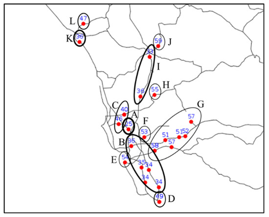
Figure 22.
The KFCx influence score (the numbers within the figure) necessary for the optimal store location identified by proposed approach query matches real-world KFC branch.
8. Conclusions
Finding suitable locations for new stores of a growing firm is a common spatial query application. However, no existing queries consider both PPOIs and NPOIs in a road network environment. We therefore proposed a novel query called the LBSN-based optimal store location query. We used check-in data and user profiles from LBSN datasets to calculate the influence score of each store in the query. This influence score and road distance were then used to identify the optimal location for a new store. We designed three algorithms for this query. The baseline algorithm first finds the solution from infinite locations in the road network. The AP algorithm then prunes areas that have no chance of holding the optimal solution to reduce the search space. The third algorithm is based on the AP algorithm; it further prunes road segments that have no chance of holding the optimal solution, increasing efficiency even further. We conducted a series of experiments to verify the efficacy of the proposed approach.
In future work, we plan to make the following extensions: (1) The method proposed in this paper only searches for one optimal solution at a time; to find multiple optimal solutions, the user must operate the algorithm multiple times. Therefore, we plan to merge the concept of the top-k query or the skyline query with the proposed approach. (2) This paper only considered the influences between existing POIs and the new store. However, there are many other factors, such as transportation, rent, land use, or licenses, which are relevant to the proposed problem. Therefore, we plan to expand the scope of the approach to include these factors.
Author Contributions
Conceptualization, Yen-Hsun Lin and Yi-Chung Chen; data curation, Yen-Hsun Lin; formal analysis, Yen-Hsun Lin; funding acquisition, Yi-Chung Chen and Chiang Lee; investigation, Yen-Hsun Lin, Yi-Chung Chen and Sheng-Min Chiu; methodology, Yen-Hsun Lin; project administration, Yi-Chung Chen and Chiang Lee; resources, Yen-Hsun Lin; software, Yen-Hsun Lin; supervision, Yi-Chung Chen and Chiang Lee; validation, Sheng-Min Chiu and Fu-Cheng Wang; visualization, Fu-Cheng Wang; writing—original draft, Yen-Hsun Lin, Yi-Chung Chen, Sheng-Min Chiu and Fu-Cheng Wang; writing—review & editing, Yi-Chung Chen, Sheng-Min Chiu and Fu-Cheng Wang. All authors have read and agreed to the published version of the manuscript.
Funding
This study was supported by the Research Assistantships funded by the Ministry of Science and Technology, Taiwan (grant number MOST 110-2121-M-224-001, to Y.-C.C.; MOST110-2221-E-006-176, to C.L.).
Data Availability Statement
The research data set of the experiment can be found on OpenStreetMap.
Acknowledgments
The authors would like to thank Ruth Li for her time and effort in meticulously proofreading and editing the paper.
Conflicts of Interest
The authors declare no conflict of interest.
Appendix A. Example of Baseline Algorithm
Figure A1a displays a roadmap with 9 points and 12 edges. The values in the parentheses represent the lengths of the edges. Suppose the customer similarity score matrix calculated by the system is
and the query user provides PPOI set {p1, p2}, NPOI set {p3}, and RPOI set {p3}. The locations of these POIs are indicated in Table A1.
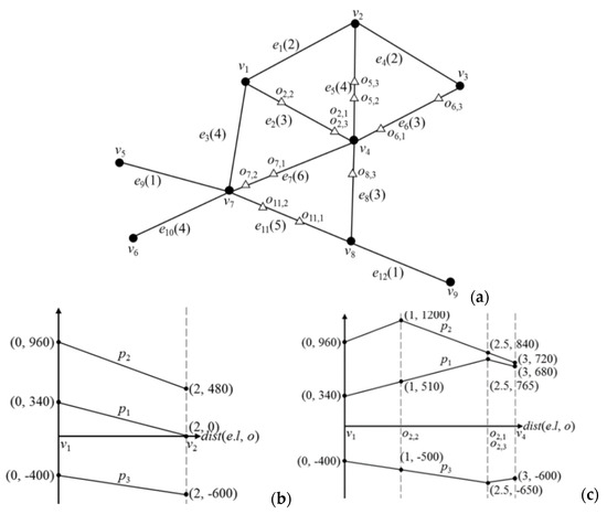
Figure A1.
Example of the baseline algorithm: (a) road network; (b) graph of disp(p,o) × CI(Q, p) on e1; (c) graph of disp(p,o) ×CI(Q, p) on e2.
Figure A1.
Example of the baseline algorithm: (a) road network; (b) graph of disp(p,o) × CI(Q, p) on e1; (c) graph of disp(p,o) ×CI(Q, p) on e2.
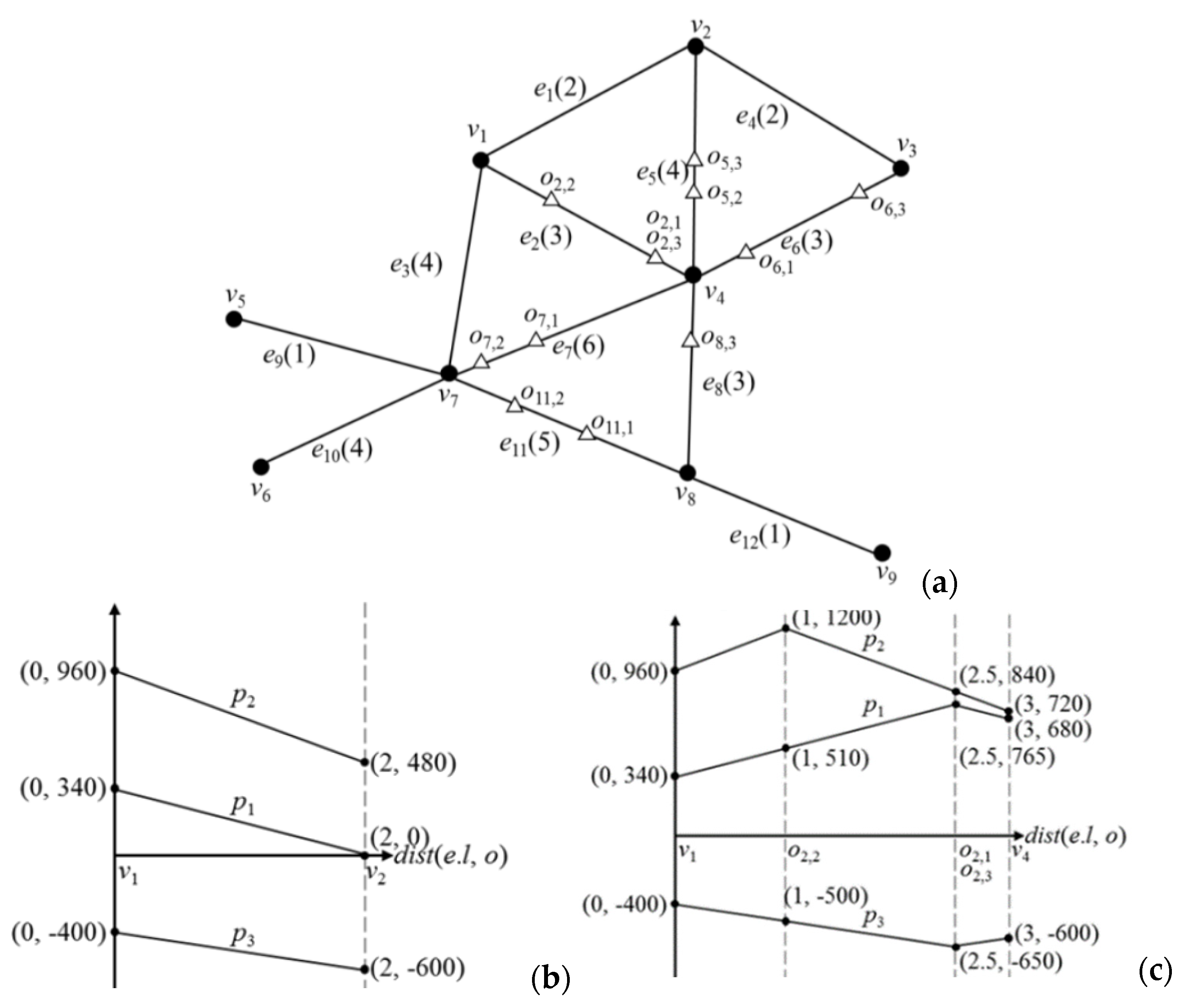

Table A1.
Information of Pp and Pn.
Table A1.
Information of Pp and Pn.
| Set | POI | Location | Impact of POI |
|---|---|---|---|
| Pp | p1 | v2 | 170 |
| p2 | v3 | 240 | |
| Pn | p3 | v7 | −100 |
In Step 1, the system calculates the influence score of the POIs: CI(Q, p1) = (170)/1 = 170, CI(Q, p2) = (240)/1 = 240, and CI(Q, p3) = −(100)/1 = −100. Thus, the influence score of p1, p2, and p3 are 170, 240, and −100, as shown in Table A1.
In Step 2, the system calculates the break points of all edges. The dist(p,o) of e1 is as shown in Figure A1b. The system identifies that the vertices of e1 are v1 and v2 and that there are no break points on e1. The dist(p,o) of e2 is as shown in Figure A1c. The system identifies that the vertices of e1 are v1 and v4 and that the break points on e1 are o2,1, o2,2, and o2,3. The remaining edges are analyzed similarly. All vertices are as shown in Table A2. All of the break points are as shown in Table A3, with ox,y indicating that py is at a break point on ex.

Table A2.
List of vertices.
Table A2.
List of vertices.
| Edge | Left Vertex | Right Vertex |
|---|---|---|
| e1 | v1 | v2 |
| e2 | v1 | v4 |
| e3 | v1 | v7 |
| e4 | v2 | v3 |
| e5 | v2 | v4 |
| e6 | v3 | v4 |
| e7 | v4 | v7 |
| e8 | v4 | v8 |
| e9 | v5 | v7 |
| e10 | v6 | v7 |
| e11 | v7 | v8 |
| e12 | v8 | v9 |

Table A3.
List of break points.
Table A3.
List of break points.
| Edge | Break Point | dist(e.l, Bp) |
|---|---|---|
| e2 | o2,1 | 2.5 |
| o2,2 | 1 | |
| o2,3 | 2.5 | |
| e5 | o5,2 | 2.5 |
| o5,3 | 2 | |
| e5 | o6,1 | 2.5 |
| o6,3 | 0.5 | |
| e7 | o7,1 | 4 |
| o7,2 | 5.5 | |
| e7 | o8,3 | 1 |
| e11 | o11,1 | 3 |
| o11,2 | 1.5 |
In Step 3, the system calculates the location scores of all break points and vertices. With vertex v1 as an example, LS(o2,1, pP, nP) = 340 + 960 + (−400) = 900. With break point o2,1 as an example, LS(o2,1, pP, nP) = 765 + 840 + (−650) = 955. The location scores of the remaining vertices and break points are calculated similarly. Table A4 exhibits a complete list of the location scores, among which that of v3 is the lowest. The system thus responds with the solution v3.

Table A4.
List of location scores of vertices and break points.
Table A4.
List of location scores of vertices and break points.
| Point | dist(p1, Point) × CI(Q, p1) | dist(p2, Point) × CI(Q, p2) | dist(p3, Point) × CI(Q, p3) | Location Score | Point | dist(p1, Point) × CI(Q, p1) | dist(p2, Point) × CI(Q, p2) | dist(p3, Point) × CI(Q, p3) | Location Score |
|---|---|---|---|---|---|---|---|---|---|
| o2,1 | 765 | 840 | −650 | 955 | o11,2 | 1275 | 2280 | −150 | 3405 |
| o2,2 | 510 | 1200 | −500 | 1210 | v1 | 340 | 960 | −400 | 900 |
| o2,3 | 765 | 840 | −650 | 955 | v2 | 0 | 480 | −600 | −120 |
| o5,2 | 425 | 1080 | −750 | 755 | v3 | 340 | 0 | −800 | −460 |
| o5,3 | 340 | 960 | −800 | 500 | v4 | 680 | 720 | −600 | 800 |
| o6,1 | 765 | 600 | −650 | 715 | v5 | 1190 | 2160 | −100 | 3250 |
| o6,3 | 425 | 120 | −850 | −305 | v6 | 1700 | 2880 | −400 | 4180 |
| o7,1 | 1360 | 1680 | −200 | 2840 | v7 | 1020 | 1920 | 0 | 2940 |
| o7,2 | 1105 | 2040 | −50 | 3095 | v8 | 1190 | 1440 | −500 | 2130 |
| o8,3 | 850 | 960 | −700 | 1110 | v9 | 1360 | 1680 | −600 | 2440 |
| o11,1 | 1530 | 1920 | −300 | 3150 |
Appendix B. Proof of Theorem A1
Theorem A1.
Consider the query set (pP, nP, rP), where p is a POI in pP and nP. Location o is any given point on any given edge in Gi. The best location score in Gi must be greater than or equal to the sum of all LB(Gi, p):
Proof.
To first prove that dist(o,p) × CI(Q, p) ≥ LB(Gi, p), we let o belong to edge e. This results in four cases depending on the two conditions, as depicted in Table A5: (1) Is CI(Q, p) greater than or equal to 0? (2) Does p belong to Gi?

Table A5.
Four cases of Theorem A1.
Table A5.
Four cases of Theorem A1.
| p Is Not in Gi | p Is in Gi | |
|---|---|---|
| CI(Q, p) ≥ 0 | Case 1 | Case 2 |
| CI(Q, p) < 0 | Case 3 | Case 4 |
Case 1. CI(Q, p) ≥ 0 and p does not belong to Gi. This case can be divided into four subcases depending on two conditions. We let dist(o,e.l) be yl and dist(o,e.r) be yr. As shown in Table A6, the two conditions are as follows: (1) Is yl less than or equal to yr? (2) Are there any break points on e? The graphs of the four dist(o,p)×CI(Q, p) are presented in Figure A2. The x axis is dist(o,e.l), and the y axis is dist(o,p) × CI(Q, p). The minimum values of Cases 1.1 and 1.3 are CI(Q, p) × yl, and the minimum values of Cases 1.2 and 1.4 are CI(Q, p) × yr.

Table A6.
Four subcases of Case 1.
Table A6.
Four subcases of Case 1.
| yl ≤ yr | yl > yr | |
|---|---|---|
| Break point on e | Case 1.1 | Case 1.2 |
| No break point on e | Case 1.3 | Case 1.4 |

Figure A2.
dist(o,p) × CI(Q, p) graphs for Case 1: (a) case 1.1, (b) case 1.2, (c) case 1.3, and (d) case 1.4.
Figure A2.
dist(o,p) × CI(Q, p) graphs for Case 1: (a) case 1.1, (b) case 1.2, (c) case 1.3, and (d) case 1.4.

In Cases 1.1–1.4, lowDist(Gi, p) is a non-negative number less than or equal to the distance from p to any given vertex in Gi; thus, lowDist(Gi, p) ≤ yl, yr, which means that lowDist(Gi, p) ≤ dist(o,p). Because CI(Q, p) ≥ 0, CI(Q, p) × lowDist(Gi, p) = LB(Gi, p) ≤ CI(Q, p) × dist(o,p).
Case 2. CI(Q, p) ≥ 0 and p belongs to Gi. This case can be divided into eight subcases depending on three conditions. Again, we let dist(o,e.l) be yl and dist(o,e.r) be yr. As shown in Table A7, the three conditions are as follows: (1) Is o on e? (2) Are there any Break points on e? (3) Is yl less than or equal to yr?

Table A7.
Eight subcases of Case 2.
Table A7.
Eight subcases of Case 2.
| o Is Not on e | Break Point on e | y1 ≥ y2 | Subcase |
|---|---|---|---|
| True | True | True | Case 2.1 |
| True | True | False | Case 2.2 |
| True | False | True | Case 2.3 |
| True | False | False | Case 2.4 |
| False | True | True | Case 2.5 |
| False | True | False | Case 2.6 |
| False | False | True | Case 2.7 (does not exist) |
| False | False | False | Case 2.8 (does not exist) |
The graphs of the eight dist(o,p) × CI(Q, p) are as displayed in Figure A3. The x axis is dist(o,e.l) and the y axis is dist(o,p) × CI(Q, p). The minimum values of Cases 2.1 and 2.3 are CI(Q, p) × yl, the minimum values of Cases 2.2 and 2.4 are CI(Q, p) × yr, and the minimum values of Cases 2.5 and 2.6 are 0. Cases 2.7 and 2.8 do not exist because o is a break point on e.

Figure A3.
dist(o,p) × CI(Q, p) graphs for Case 2: (a) case 2.1, (b) case 2.2, (c) case 2.3, (d) case 2.4, (e) case 2.5, and (f) case 2.6.
Figure A3.
dist(o,p) × CI(Q, p) graphs for Case 2: (a) case 2.1, (b) case 2.2, (c) case 2.3, (d) case 2.4, (e) case 2.5, and (f) case 2.6.

The proofs of Cases 2.1–2.4 are identical to those of Cases 1.1–1.4. In Cases 2.5–2.6, lowDist(Gi, p) is a non-negative number less than or equal to the distance from p to any given vertex in Gi; in addition, p belongs to Gi, and dist(p,p) = 0. Thus, lowDist(Gi, p) ≤ 0 ≤ dist(o,p). Because CI(Q, p) ≥ 0, CI(Q, p) × lowDist(Gi, p) = LB(Gi,p) ≤ CI(Q, p) × dist(o,p).
Case 3. CI(Q, p) < 0 and p does not belong to Gi. This case can be divided into four subcases depending on two conditions. Again, we let dist(o,e.l) be yl and dist(o,e.r) be yr. As shown in Table A8, the two conditions are as follows: (1) Are there any break points on e? (2) Is yl less than or equal to yr?

Table A8.
Four subcases of Case 3.
Table A8.
Four subcases of Case 3.
| yl ≤ yr | yl > yr | |
|---|---|---|
| Break point on e | Case 3.1 | Case 3.2 |
| No break point on e | Case 3.3 | Case 3.4 |
The graphs of the four dist(o,p) × CI(Q, p) are as presented in Figure A4. The x axis represents dist(o,e.l), and the y axis represents dist(o,p) × CI(Q, p). The minimum value of Case 3.1 is CI(Q, p) × yl, and the minimum value of Case 3.2 is CI(Q, p) × yr. By solving simultaneous equations, we can derive that the minimum values of Cases 3.3 and 3.4 are CI(Q, p) × ((y1 + y2 + e.length)/2).

Figure A4.
dist(o,p) × CI(Q, p) graphs for Case 3: (a) case 3.1, (b) case 3.2, (c) case 3.3, and (d) case 3.4.
Figure A4.
dist(o,p) × CI(Q, p) graphs for Case 3: (a) case 3.1, (b) case 3.2, (c) case 3.3, and (d) case 3.4.

In Case 3.1, highDist(Gi,p) is a non-negative number greater than or equal to the distance from p to any given vertex in Gi; thus, highDist (Gi,p) ≥ yl, which means that highDist (Gi,p) ≥ dist(o,p). Because CI(Q, p) < 0, LB(Gi, p) = CI(Q, p) × (highDist(Gi, p) + maxEdge(Gi)/2) ≤ CI(Q, p) × highDist(Gi,p) ≤ CI(Q, p) × dist(o,p).
In Case 3.2, highDist(Gi,p) is a non-negative number greater than or equal to the distance from p to any given vertex in Gi; thus, highDist (Gi,p) ≥ yr, which means that highDist (Gi,p) ≥ dist(o,p). Because CI(Q, p) < 0, LB(Gi, p) = CI(Q, p) × (highDist(Gi, p) + maxEdge(Gi)/2) ≤ CI(Q, p) × highDist(Gi,p) ≤ CI(Q, p) × dist(o,p).
In Cases 3.3–3.4, highDist(Gi,p) is a non-negative number greater than or equal to the distance from p to any given vertex in Gi and maxEdge(Gi) is the length of the longest edge in Gi. Thus,
Case 4. CI(Q, p) < 0 and p belongs to Gi. Case 4 can be divided into eight subcases depending on three conditions. Again, we let dist(o,e.l) be yl and dist(o,e.r) be yr. As shown in Table A9, the three conditions are as follows: (1) Is o on e? (2) Are there any break points on e? (3) Is yl less than or equal to yr?

Table A9.
Eight subcases of Case 4.
Table A9.
Eight subcases of Case 4.
| o Is Not on e | No Break Point on e | y1 ≤ y2 | Subcase |
|---|---|---|---|
| True | True | True | Case 4.1 |
| True | True | False | Case 4.2 |
| True | False | True | Case 4.3 |
| True | False | False | Case 4.4 |
| False | True | True | Case 4.5 (does not exist) |
| False | True | False | Case 4.6 (does not exist) |
| False | False | True | Case 4.7 |
| False | False | False | Case 4.8 |
The graphs of the eight dist(o,p) × CI(Q, p) are as displayed in Figure A5. The x axis represents dist(o,e.l), and the y axis represents dist(o,p) × CI(Q, p). Cases 4.5 and 4.6 do not exist because o is a break point on e. The proofs of Cases 4.1–4.4 are identical to those of Cases 3.1–3.4. The proofs of Cases 4.7 and 4.8 are identical to those of Cases 4.1 and 4.2.

Figure A5.
dist(o,p) × CI(Q, p) graphs for Case 4: (a) case 4.1, (b) case 4.2, (c) case 4.3, (d) case 4.4, (e) case 4.7, and (f) case 4.8.
Figure A5.
dist(o,p) × CI(Q, p) graphs for Case 4: (a) case 4.1, (b) case 4.2, (c) case 4.3, (d) case 4.4, (e) case 4.7, and (f) case 4.8.

Through Cases 1–4, we have proven that dist(o,p) × CI(Q, p) ≥ LB(Gi, p), and since o is any given point on any given edge in Gi, we can derive that
Appendix C. Proof of Theorem A2
Theorem A2.
lowDist(Gi, u) must be a non-negative number less than or equal to the distance from u to any given vertex in Gi.
Proof.
We formulated the proof using two cases:
- Case 1. u belongs to Gi. The minimum distance between any two points is 0 because lowDist(Gi,u) = 0 ≤ 0.
- Case 2. u does not belong to Gi. As indicated by [28],
Any path from u to v must pass through a series of G+-tree nodes Gx(u), Gx−1(u), …, G1(u), G1(v), G2(v), …, Gx(v). To calculate the road distance from u to any given point in Gi, we pass through Gx(u), Gx−1(u), …, Gi. Since u does not belong to Gi, Gi is not one of the nodes between Gx(u) and G1(u). As shown in Figure 7, if we let Gi equal Gn(v), then we pass through the same series of G-tree nodes, Gx(u), Gx−1(u), …, G1(u), …, Gn(v). Thus, the minimum road distance from u to any given point in Gi, can be expressed as follows:
where the summation of the last three terms must be greater than or equal to
which represents low(Gn(v)). Therefore, we can re-write Equation (A6) as follows:
The right side of this equation equals lowDist(Gi, u). Thus, we can prove that
□
Appendix D. Proof of Theorem A3
Theorem A3.
highDist(Gi, u) must be a non-negative number greater than or equal to the distance from u to any given vertex in Gi.
Proof.
We formulated the proof using two cases:
Case 1. u does not belong to Gi
Based on Figure 8, as with Case 2 of Theorem A2, if we let Gi equal Gn(v), then we pass through the same series of G+-tree nodes, Gx(u), Gx−1(u), …, G1(u), …, Gn(v). Thus, the maximum road distance from u to any given point in Gi can be expressed as follows:
where the summation of the last four terms is less than or equal to
This is equal to high(Gn(v)). Finally, after we substitute high(Gn(v)) into Equation (A10), the right side of Equation (A10) equals highDist(Gi, u). Therefore, we can obtain maxv∈Gidist(u, v) ≤ highDist(Gi, u).
Case 2. u belongs to Gi
As u belongs to Gi, as shown in Figure 9, the shortest path from u to v must pass through a series of G+-tree nodes Gx(u), Gx−1(u), …, Gm+1(u), Gm+1(v), …, Gx(v), in which we use Gm(u) or Gm(v) to express LCA(u, v). LCA(u, v) varies with v, and m may be among 1 − x. As shown in Figure A6, we let a path from u to v be farPath(u, v), which must pass through Gx(u), Gx−1(u), …, G1(u), G1(v), G2(v), …, Gx(v). The length of farPath(u, v) must be greater than or equal to shortestPath(u,v). Therefore, maxv∈Gidist(u, v) ≤ maxv∈GifarPath(u, v).

Figure A6.
farPath(u, v) and shortestPath(u, v).
Figure A6.
farPath(u, v) and shortestPath(u, v).
The maximum road distance from u to any given point in Gi can be expressed as follows:
where the summation of the last six terms is less than or equal to
This is less than or equal to high(G1(v)). Thus, we can re-write Equation (A12) as follows:
Finally, after we substitute Equation (A14) into Equation (A12), the right side of Equation (A12) equals highDist(Gi, u). Thus, we can re-write Equation (A12) as maxv∈Gidist(u, v) ≤ highDist(Gi, u). □
Appendix E. Example of AP algorithm
We used the example presented in Figure A2 to demonstrate the AP algorithm. The G+-tree is presented in Figure A7. The extra information in each G+-tree node is as shown in Table A10, and the vertices and edges in the G+-tree nodes are displayed in Table A11. Suppose the query user inputs PPOI set {p1, p2}, NPOI set {p3}, and RPOI set {p3}. The locations of these POIs on the roadmap are exhibited in Table A6.

Figure A7.
Example of the AP algorithm procedure.
Figure A7.
Example of the AP algorithm procedure.
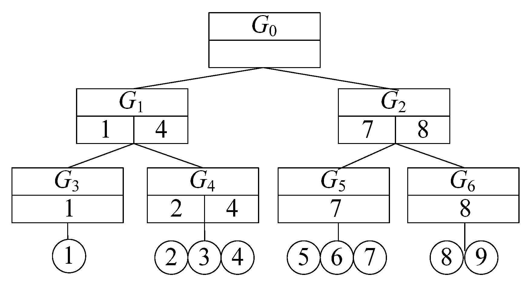

Table A10.
Additional information in the G+-tree nodes.
Table A10.
Additional information in the G+-tree nodes.
| G+ Tree Node Gi | Low(Gi) | High(Gi) | maxEdge(Gi) |
|---|---|---|---|
| G1 | 0 | 8 | 6 |
| G2 | 0 | 9 | 5 |
| G3 | 0 | 0 | 4 |
| G4 | 0 | 4 | 6 |
| G5 | 0 | 4 | 6 |
| G6 | 0 | 1 | 1 |

Table A11.
Vertices and edges in the G+-tree nodes.
Table A11.
Vertices and edges in the G+-tree nodes.
| G+ Tree Nod Gi | Vertices in Gi | Edges in Gi |
|---|---|---|
| G1 | v1, v2, v3, v4 | e1, e2, e3, e4, e5, e6, e7, e8 |
| G2 | v5, v6, v7, v8, v9 | e9, e10, e11, e12 |
| G3 | v1 | e1, e2, e3 |
| G4 | v2, v3, v4 | e4, e5, e6, e7, e8 |
| G5 | v5, v6, v7 | e9, e10, e11 |
| G6 | v8, v9 | e12 |
In Step 1, the system calculates the influence score of the POIs. The process is identical to that in Step 1 of the baseline algorithm. In Step 2, the system begins to visit the G+-tree, as shown in Table A12.

Table A12.
Procedure of the G+-tree traversal.
Table A12.
Procedure of the G+-tree traversal.
| Iteration | Node Gi Which Is Being Visited | Action | Current Answer (Location Score) |
|---|---|---|---|
| 1 | G0 | Traversing is continued. | Null (+∞) |
| 2 | G1 | Traversing is continued. | Null (+∞) |
| 3 | G3 | Calculating the location score of v1, v2, v4, v7, o2.1, o2.2, o2.3, and traversing is continued. | V2 (−120) |
| 4 | G4 | Calculating the location score of v2, v3, v4, v7, v8, o5.2, o5.3, o6.1, o7.1, o7.2, o8.3, and traversing is continued. | V3 (−460) |
| 5 | G2 | Pruning G2, and traversing is finished. Return the answer. |
In Round 1, root node G0 is visited first. As no location scores have been calculated yet, G0 cannot be pruned. G0 is a non-leaf node, so we return to Step 2 and continue visiting the G+-tree.
In Round 2, G1 is visited. As no location scores have been calculated yet, G1 cannot be pruned. G1 is a non-leaf node, so we return to Step 2 and continue visiting the G+-tree.
In Round 3, G3 is visited. As no location scores have been calculated yet, G3 cannot be pruned. G3 is a leaf node, so the system finds the break points and vertices of all edges in G3. As shown in Table A11, the edges in G3 include e1, e2, and e3. The system finds all of the break points and vertices on e1, e2, and e3, which include v1, v2, v4, v7, o2.1, o2.2, and o2.3, and then calculates the location scores of these points. The process is identical to that of Steps 2 and 3 of the baseline algorithms. At present, the optimal solution is v2, the location score of which is −120. We return to Step 2 and continue visiting the G+-tree.
In Round 4, G4 is visited. As shown in Table A13 ∑p∈pP∪npLB(G4, p) = 0 + 0 + (−1300) = −1300 < −120, which means that G4 cannot be pruned. The edges in G4 include e4, e5, e6, e7, and e8. The system finds all of the break points and vertices on these edges, which include v2, v3, v4, v7, v8, o5.2, o5.3, o6.1, o6.3, o7.1, o7.2, and o8.3. It then calculates the location scores of these points. At present, the optimal solution is v3, the location score of which is −460. We return to Step 2 and continue visiting the G+-tree.

Table A13.
lowDist, highDist, and LB of G+-tree nodes.
Table A13.
lowDist, highDist, and LB of G+-tree nodes.
| G+ Tree Node Gi | lowDist (Gi, v2) | lowDist (Gi, v3) | lowDist (Gi, v7) | highDist (Gi, v2) | highDist (Gi, v3) | highDist (Gi, v7) | LB (Gi, v2) | LB (Gi, v3) | LB (Gi, v7) |
|---|---|---|---|---|---|---|---|---|---|
| G1 | 0 | 0 | 4 | 10 | 11 | 12 | 0 | 0 | −1500 |
| G2 | 6 | 6 | 0 | 15 | 15 | 9 | 1020 | 1440 | −1150 |
| G3 | 2 | 4 | 4 | 2 | 4 | 4 | 340 | 960 | −600 |
| G4 | 0 | 0 | 6 | 4 | 6 | 10 | 0 | 0 | −1300 |
| G5 | 6 | 8 | 0 | 10 | 12 | 4 | 1020 | 1920 | −700 |
| G6 | 7 | 6 | 5 | 8 | 7 | 6 | 1190 | 1440 | −650 |
In Round 5, G2 is visited, and ∑p∈pP∪npLB(G2, p = 1020 + 1440 + (−1150) = 1310 > −460; thus, G2 is pruned. The entire G+-tree has been visited, so the optimal location for the new store is v3.
Appendix F. Proof of Theorem A4
Theorem A4.
Consider edge e and query set (pP, nP, rP). We refer to nP∪rP as POIs. We use BP(p,e) to represent a break point of POI p on e and use BPs(POIs,e) to represent a set of all p on e in the POIs. Thus, we have the following:
where the former term is the best location score on e; the latter can be regarded as the lower bound of this location score.
Proof.
Intuitively, we can see the following is true:
where the right side of the inequality also equals .
In the proof of Theorem 1, we showed that dist(o,p)×CI(Q, p) is a linear function or a piecewise linear function and that its minimum value must be at a vertex {e.l, e.r} of e or at BP(p, e) of p on e. Thus, Equation (A16) can be re-written as follows:
□
Appendix G. Example of the AEP Algorithm
We illustrate the AEP algorithm using the example presented in Figure A2. Suppose the query user inputs PPOI set {p1, p2}, NPOI set {p3}, and RPOI set {p3}. The locations of these POIs on the roadmap are exhibited in Table A6. Table A14 presents the lower bounds of each edge. We refer to as eLB(e,p) and to as eLB(e).

Table A14.
Lower bound of the edges.
Table A14.
Lower bound of the edges.
| Edge | eLB(e,p1) | eLB(e,p2) | eLB(e,p3) | eLB(e) | Edge | eLB(e,p1) | eLB(e,p2) | eLB(e,p3) | eLB(e) |
|---|---|---|---|---|---|---|---|---|---|
| e1 | 0 | 480 | −600 | −120 | e7 | 680 | 720 | −600 | 800 |
| e2 | 340 | 720 | −650 | 410 | e8 | 680 | 720 | −700 | 700 |
| e3 | 340 | 720 | −600 | 460 | e9 | 1020 | 1920 | −100 | 2840 |
| e4 | 0 | 0 | −800 | −800 | e10 | 1020 | 1920 | −400 | 2540 |
| e5 | 0 | 480 | −800 | −320 | e11 | 1020 | 1440 | −500 | 1960 |
| e6 | 340 | 0 | −850 | −510 | e12 | 1190 | 1440 | −600 | 2030 |
The execution process of the AEP algorithm is similar to that of the AP algorithm. As shown in Table A15, the only differences occur in Rounds 3 and 4 of visiting the G+-tree.

Table A15.
Traversal of the G+-tree.
Table A15.
Traversal of the G+-tree.
| Iteration | Node Gi Which Is Being Visited | The Edge e Which Is Being Visited | Action | Current Answer (Location Score) |
|---|---|---|---|---|
| 1 | G0 | Traversing is continued. | null (+∞) | |
| 2 | G1 | Traversing is continued. | null (+∞) | |
| 3 | G3 | e1 | Calculating the location score of v1, v2 | v2 (−120) |
| e2 | Pruning e2 | v2 (−120) | ||
| e3 | Pruning e3 | v2 (−120) | ||
| 4 | G4 | e4 | Calculating the location score of v2, v3 | v3 (−460) |
| e5 | Pruning e5 | v3 (−460) | ||
| e6 | Pruning e6 | v3 (−460) | ||
| e7 | Pruning e7 | v3 (−460) | ||
| e8 | Pruning e8 | v3 (−460) | ||
| 5 | G2 | Pruning G2, and traversing is finished. |
In Round 3, the system visits G3. As shown in Table A15, the edges in G3 include e1, e2, and e3. The system visits them sequentially. First, the system visits e1. As no location scores have been calculated yet, e1 cannot be pruned. The system finds all of the break points and vertices on e1, which include v1 and v2, and then calculates the location scores of these points. The process is identical to that of Steps 2 and 3 of the baseline algorithm. At present, the optimal solution is v2, the location score of which is −120. Next, the system visits e2. As shown in Table A14, eLB(e2) = 340 + 720 + (−650) = 410 > −120. Thus, e2 is pruned. Next, the system visits e3: eLB(e3) = 340 + 720 + (−600) = 460 > −120. Thus, e3 is pruned.
In Round 4, the system visits G4. The edges in G4 include e4, e5, e6, e7, and e8. First, the system visits e4. eLB(e4) = 0 + 0 + (−800) = −800 < −120, which means that e4 cannot be pruned. The system finds all of the break points and vertices on e4, which include v2 and v3, and then calculates the location scores of these points. At present, the optimal solution is v3, the location score of which is −460. The system next visits e5, e6, e7, and e8. These edges are pruned in a similar manner.
References
- Zhang, J.; Ku, W.-S.; Sun, M.; Qin, X.; Lu, H. Multi-criteria optimal location query with overlapping voronoi diagrams. In Proceedings of the 17th International Conference on Extending Database Technology (EDBT), Edinburgh, UK, 29 March–1 April 2014; pp. 391–402. [Google Scholar]
- Arvanitis, A.; Deligiannakis, A.; Vassiliou, Y. Efficient influence-based processing of market research queries. In Proceedings of the 21st ACM International Conference on Information and Knowledge Management, Maui, HI, USA, 29 October–2 November 2012; pp. 1193–1202. [Google Scholar]
- Xiao, X.; Yao, B.; Li, F. Optimal location queries in road network databases. In Proceedings of the 2011 IEEE 27th International Conference on Data Engineering, Washington, DC, USA, 11–16 April 2011; pp. 804–815. [Google Scholar]
- Lee, C. Finding the k-Most Suitable Locations under Minimum Average Distance. Master’s Thesis, National Cheng-Kung University, Tainan, Taiwan, 2015. [Google Scholar]
- Lin, Y.; Wang, E.T.; Chiang, C.; Chen, A.L.P. Finding targets with the nearest favor neighbor and farthest disfavor neighbor by a skyline query. In Proceedings of the 29th Annual ACM Symposium on Applied Computing, Gyeongju, Korea, 24–28 March 2014; pp. 821–826. [Google Scholar]
- Sacharidis, D.; Deligiannakis, A. Spatial cohesion queries. In Proceedings of the 23rd SIGSPATIAL International Conference on Advances in Geographic Information Systems, Beijing, China, 2–5 November 2015; pp. 1–10. [Google Scholar]
- Qi, J.; Zhang, R.; Kulik, L.; Lin, D.; Xue, Y. The min-dist location selection query. In Proceedings of the 2012 IEEE 28th International Conference on Data Engineering, Arlington, VA, USA, 2–5 April 2012; pp. 366–377. [Google Scholar]
- Su, I.; Huang, Y.; Chung, Y.; Shen, I. Finding both aggregate nearest positive and farthest negative neighbors. In Proceedings of the International Conference on Information and Knowledge Engineering (IKE), Las Vegas, NV, USA, 16–19 July 2012. [Google Scholar]
- Foursquare. Available online: https://foursquare.com/ (accessed on 17 February 2022).
- Facebook. Available online: https://www.facebook.com/ (accessed on 17 February 2022).
- Chen, Y.C.; Huang, H.H.; Chiu, S.M.; Lee, C. Joint Promotion Partner Recommendation Systems Using Data from Location-Based Social Networks. ISPRS Int. J. Geo-Inf. 2021, 10, 57. [Google Scholar] [CrossRef]
- Yin, D.; Mitra, S.; Zhang, H. Research Note—When Do Consumers Value Positive vs. Negative Reviews? An Empirical In-vestigation of Confirmation Bias in Online Word of Mouth. Inf. Syst. Res. 2016, 27, 131–144. [Google Scholar] [CrossRef]
- Kang, L.; Liu, S.; Gong, D.; Tang, M. A personalized point-of-interest recommendation system for O2O commerce. Electron. Mark. 2022, 31, 253–267. [Google Scholar] [CrossRef]
- Chen, Z.; Liu, Y.; Wong, R.C.; Xiong, J.; Mai, G.; Long, C. Efficient algorithms for optimal location queries in road networks. In Proceedings of the 2014 ACM SIGMOD International Conference on Management of Data, Snowbird, UT, USA, 22–27 June 2014; pp. 123–134. [Google Scholar]
- Xu, L.; Mai, G.; Chen, Z.; Liu, Y.; Dai, G. Minsum based optimal location query in road networks. In Proceedings of the International Conference on Database Systems for Advanced Applications, Suzhou, China, 27–30 March 2017; pp. 441–457. [Google Scholar]
- Zhao, J.; Yang, S.; Huo, H.; Sun, Q.; Geng, X. TBTF: An effective time-varying bias tensor factorization algorithm for recommender system. Appl. Intell. 2021, 51, 4933–4944. [Google Scholar] [CrossRef]
- Cui, L.; Wang, X. A Cascade Framework for Privacy-Preserving Point-of-Interest Recommender System. Electronics 2022, 11, 1153. [Google Scholar] [CrossRef]
- Galal, S.; Nagy, N.; El-Sharkawi, M.E. CNMF: A Community-Based Fake News Mitigation Framework. Information 2021, 12, 376. [Google Scholar] [CrossRef]
- Li, H.; Hong, R.; Zhu, S.; Ge, Y. Point-of-interest recommender systems: A separate-space perspective. In Proceedings of the 2015 IEEE International Conference on Data Mining, Atlantic City, NJ, USA, 14–17 November 2015; pp. 231–240. [Google Scholar]
- Bao, J.; Zheng, Y.; Mokbel, M.F. Location-based and preference-aware recommendation using sparse geo-social networking data. In Proceedings of the 20th International Conference on Advances in Geographic Information Systems, Redondo Beach, CA, USA, 6–9 November 2012; pp. 199–208. [Google Scholar]
- Hsieh, H.; Li, C.; Lin, S. Triprec: Recommending trip routes from large scale check-in data. In Proceedings of the 21st International Conference on World Wide Web, Lyon, France, 16–20 April 2012; pp. 529–530. [Google Scholar]
- Lu, E.H.; Chen, C.; Tseng, V.S. Personalized trip recommendation with multiple constraints by mining user check-in behaviors. In Proceedings of the 20th International Conference on Advances in Geographic Information Systems, Redondo Beach, CA, USA, 6–9 November 2012; pp. 209–218. [Google Scholar]
- Wen, Y.T.; Cho, K.J.; Peng, W.C.; Yeo, J.; Hwang, S.W. Kstr: Keyword-aware skyline travel route recommendation. In Proceedings of the 2015 IEEE International Conference on Data Mining, Atlantic City, NJ, USA, 14–17 November 2015; pp. 449–458. [Google Scholar]
- Wang, X.; Zhang, Y.; Zhang, W.; Lin, X. Distance-aware influence maximization in geo-social network. In Proceedings of the IEEE 32nd International Conference on Data Engineering (ICDE), Helsinki, Finland, 16–20 May 2016; pp. 1–12. [Google Scholar]
- Jin, X.; Han, J. Expectation maximization clustering. In Encyclopedia of Machine Learning and Data Mining; Springer: Berlin/Heidelberg, Germany, 2017; pp. 480–482. [Google Scholar]
- Jaccard, P. Étude comparative de la distribution florale dans une portion des Alpes et du Jura. Bull. Soc. Vaud. Sci. Nat. 1901, 37, 547–579. [Google Scholar] [CrossRef]
- Endres, D.M.; Schindelin, J.E. A new metric for probability distributions. IEEE Trans. Inf. Theory 2003, 49, 1858–1860. [Google Scholar] [CrossRef] [Green Version]
- Zhong, R.; Li, G.; Tan, K.L.; Zhou, L.; Gong, Z. G-tree: An efficient and scalable index for spatial search on road networks. IEEE Trans. Knowl. Data Eng. 2015, 27, 2175–2189. [Google Scholar] [CrossRef]
- Real Datasets for Spatial Databases: Road Networks and Points of Interest. Available online: https://www.cs.utah.edu/~lifeifei/SpatialDataset.htm (accessed on 17 February 2022).
- OpenStreetMap Project. Available online: https://www.openstreetmap.org/ (accessed on 14 January 2019).
Publisher’s Note: MDPI stays neutral with regard to jurisdictional claims in published maps and institutional affiliations. |
© 2022 by the authors. Licensee MDPI, Basel, Switzerland. This article is an open access article distributed under the terms and conditions of the Creative Commons Attribution (CC BY) license (https://creativecommons.org/licenses/by/4.0/).


