Abstract
Examining the complexity of urban form may help to understand human behavior in urban spaces, thereby improving the conditions for sustainable design of future cities. Metrics, such as fractal dimension, ht-index, and cumulative rate of growth (CRG) index have been proposed to measure this complexity. However, as these indicators are statistical rather than spatial, they result in an inability to characterize the spatial complexity of urban forms, such as building footprints. To overcome this problem, this paper proposes a graph-based fractality index (GFI), which is based on a hybrid of fractal theory and deep learning techniques. First, to quantify the spatial complexity, several fractal variants were synthesized to train a deep graph convolutional neural network. Next, building footprints in London were used to test the method, where the results showed that the proposed framework performed better than the traditional indices, i.e., the index is capable of differentiating complex patterns. Another advantage is that it seems to assure that the trained deep learning is objective and not affected by potential biases in empirically selected training datasets Furthermore, the possibility to connect fractal theory and deep learning techniques on complexity issues opens up new possibilities for data-driven GIS science.
1. Introduction
Mandelbrot wrote: “Clouds are not spheres, mountains are not cones, coastlines are not circles, and bark is not smooth, nor does lightning travel in a straight line” [1] (pp. 1–2). Hence, such natural phenomena cannot be accurately represented by simplified Euclidean geometry but can be described by fractal geometry. The literal meaning of “fractal” is “broken” or “irregular”. Since fractal geometry was discovered, it has been recognized that the fractal pattern exhibit patterns of “self-similarity” known as the first definition of fractal, meaning that each of the subdivisions is similar to the whole [2,3]. An example of a strictly defined self-similarity is the Sierpinski carpet, whose small pieces are exact copies of the large ones. Then, by adding some randomness when copying the large shapes, the second definition of fractal has been extended to be capable of describing real objects [1]. Both two definitions are in a statistical sense and demonstrate a power-law relationship between the number of copies and their corresponding scales, where the exponent of the power-law function equates to the so-called fractal dimension. Still, the power-law relationship is hardly observed in most natural phenomena; hence a third more relaxed definition has been proposed, the ht-index [4]. The purpose was to further extend the scope of fractal definitions by examining patterns where there are far more small features than large ones and to see how those pattern distributions are similar to power-law relationships. Therefore, the concept of the third definition is much broader and free from the spatial forms or shapes [5,6], instead emphasizing gradual change of scale.
Cities commonly exhibit fractal patterns; then termed “fractal cities” [7]. Fractals have been observed over different urban forms including street systems, land uses, urban sprawls, and building footprints [8,9,10]. Particularly, the measurement of the complexity of urban morphology is mainly manifested and delineated by building footprints. However, the fractal indicators based on the previous three definitions are not sufficient to describe the characteristics of fractals. On the one hand, all three definitions are given by statistical descriptions, rather than geometric forms. The feature of self-similarity thus is statistical rather than geometrical. Simply put, a statistically similar fractal pattern could have many spatial forms. This is because the three statistics-based definitions target a univariate variable, instead of multidimensional or multivariate ones. As suggested in Rootzén, Segers, and Wadsworth [11], a general mathematical model to fit heterogeneous distributions with multivariate variables is difficult. Such heterogeneous distributions characterize the fractals statistically as well as constrain the dimensions of variables. The first two fractal definitions, which investigate a power-law relationship between the scale and the number of scaled copies, and the third one, which describes an imbalanced distribution, are all built upon a univariate variable. However, most spatial targets, such as building footprints commonly have multiple features, including spatial distances between neighbors and individual attributes (such as sizes, orientations and shapes) that are still not well-captured by any of the fractal definitions alone. Therefore, there exists a methodological gap on how to combine both the forms, etc., and statistical features of fractals, so that better descriptive indicators from those measures can be inferred. Furthermore, due to this gap, there is also a shortage of examples of applications.
Meanwhile, for many applications graph-based models in the deep learning field have shown strength in non-Euclidean datasets [12]. Those advances provide a new opportunity to study the complexity of building footprints. First, how buildings are distributed in space can be effectively represented by graphs. The spatial distribution of buildings is often irregular, which means that the number of neighbors for each building is not equal, and therefore, cannot be represented by a fixed data structure, such as raster images. A graph, on the other hand, can represent complex relationships between buildings due to its flexible structure. In addition, by utilizing the capabilities of deep learning methods to extract multi-dimensional features, the spatial characteristics, as well as the attributes of individual buildings, can be investigated at the same time. In this way, the complexity of multiple features in building distributions might be possible to understand, which would be helpful for understanding the spatial characteristics of fractal building distributions and for inferring fractal forms.
To examine if and how it is possible to utilize and combine the advantages of both fractal and graph theory, in this study a graph-based deep learning model was constructed to show the complexity of building distributions, namely graph-based fractality index (GFI), based on their geometrical and statistical features. The three-fold contributions of this work can then be described as:
- 1.
- Introducing a new graph convolution neural network framework on irregular building distributions to describe their local spatial and attribute features for each building, as well as their global statistical features;
- 2.
- Devising a method under the second fractal definition to synthesize fractal patterns by an established square-based fractal regime, the Sierpinski carpet, that can be used as training and validation datasets;
- 3.
- Showing how the proposed GFI can compensate for the inability of either the fractal dimension or ht-index (or its derivative: cumulative rate of growth index, CRG) to integrate the fractal-related computations with both spatial and aspatial aspects.
As a consequence, we foresee new and not yet thought of applications where the two variables of a different character, namely statistical measures and spatial form, are combined to give new insights.
The remainder of this paper is organized as follows. Section 2 summarizes related work on the complexity of urban morphology and graph convolutional networks (GCN). Detailed information on the proposed methods, the synthetic variant dataset, and the training of the model is given in Section 3. Some case studies on the building footprints of the Greater London area are demonstrated in Section 4. Finally, the findings and insights are discussed in Section 5 with concluding remarks in Section 6.
2. Related Work
2.1. Complexity of Urban Morphology
Cities have long been recognized as complex systems which are large, nonlinear, and emergent from interacting components [13]. Studying the complexity of urban systems is to understand human collective behavior in the past [14], and facilitates livable urban design or invents future cities [13]. The understanding of complex urban forms and processes is the key to all the signs both in the past and future of nature [15], of which the spatial configuration of building footprints and their distributions is one of the most prominent aspects [16].
The morphological patterns of building distributions are either simple or complex. Simple patterns, such as collinear, curvilinear, or grid-like alignments have been extensively studied to facilitate map generalization in cartography [17,18,19,20] or to identify functional neighborhoods in spatial indexing [21,22,23]. These simple patterns are mostly described by geometric variables, such as distance and angles, and some morphological descriptors, such as proximity, similarity, closure, and continuity, which are based on visual variables proposed by the Gestalt theory [24]. Unlike the simple patterns, the complex patterns have hardly any specific forms to be categorized into and are limitedly described by only geometric or morphological descriptors. Such limitation is mainly due to the Euclidean geometric perspective that focuses essentially on the local, geometric details, such as those mentioned in geometric descriptors. Instead, the layout and distributions of building footprints may be better characterized by their complexity in the context of fractal geometries.
The fractal is a fragmented geometric shape, such as the British coastline, that can be subdivided into parts, each of which being similar to the whole [2]. Its complexity is given by the fractal dimension (FD) defined in the range between 0 and 2, where the higher the value is, the more the space is filled, leading to increasing homogeneity in the spatial distribution. However, some studies have shown that FD is positively correlated with the built-up density of the studied area [25,26]. This weakness implies that FD is a limited measure to characterize the complex form of distributions, in particular when investigating high-density agglomerations. The pattern of agglomerations in central Paris, for example, is delineated as a uniform dense distribution according to its FD [27]. Other empirical studies also suggest that the FD values of downtown areas approach 2, no matter with which type of agglomeration morphologies exist [28]. Comparing the variations of box-counting curves for the non-power-law distributions between the number of boxes and scales [29] cannot circumvent the inaccuracy of FD when handling high-density agglomerations. Thus, FD is too rigid [4]: 1, it requires the dataset to follow a power-law distribution, and therefore, it is not applicable to data with distributions, such as lognormal and exponential ones and 2, it cannot differentiate the complexity of a fractal in terms of the level of recursion. To solve these two problems, a more flexible index, the ht-index [4] as well as its improvements, the CRG index [30], the ratio of areas (RA) index [31], and the unified metrics 1&2 (UM1&2) [32] have been proposed. The ht-index is acquired by the operation of so-called head/tail breaks [33], which recursively partitions the head of a usually heavy-tailed statistical distribution by its mean values. The ht-index should be at least 3 for a distribution to be considered fractal. Developed from the ht-index, CRG, as well as the RA and UM1&2 indices, extend the integral form of the ht-index to a fractional one so that it can sense the minor difference that the ht-index cannot. Specifically, although the UM1&2 indices provide better interpretability than that of CRG and RA, their numerical values are still correlated with CRG (positively) and RA (negatively). The mathematical form of UM1&2, which only considers the ratio between the first head and tail of the sequence, is not as concise and consistent as the CRGs. More importantly, these indices are only statistic indicators and simply examine one aspect of the entities’ properties at a time. For example, the complexity of social hot spots in urban areas is inspected by the distances of tweets’ check-in locations [14], or the inhomogeneity of urban development in America is depicted by the size of built-up areas [34]. For spatial entities, such as building footprints that are commonly observed in the study of urban morphology, not only the statistical distribution but also the spatial relationships between neighborhoods must be considered. In addition, a comprehensive perspective that includes multivariate spatial features, e.g., the area and distance, should also be reexamined.
2.2. Graph Convolutional Networks
In recent years, deep learning has received wide attention and extensive applications both in the industry and academia. It has proven to be successful in the areas, such as pattern recognition and classification in uniformly structured data, such as images, audio, and texts [35]. Additionally, applications of various deep learning models are becoming increasingly used in the analysis of spatio-temporal predictions, commonly seen in the field of traffic and transportation [36,37,38], ecology [39], and economics [40]. Yet, most natural phenomena or decentralized systems are heterogeneous, and they are represented by irregularly structured graphs, such as social network graphs and traffic trajectories [41]. Developing efficient models to analyze irregular graph-based datasets has, therefore, attracted significant attention in the field of deep learning.
In deep learning, the most successful feature detector is the convolution operation. Simply put, the process of convolution is to compare and aggregate the differences between the central object and its neighbors. Based on this technique, the graph convolutional network (GCN) extracts graph features in two spaces: the spatial domain [42] and the spectral domain [43]. In the spatial domain, the convolution operation is directly applied to individual vertices and their neighborhoods. The design of the convolution kernel function determines the distance of the neighbors to be considered. This approach is much like the spatial operations on regularly structured data formats. Like the traditional convolution operation, designing fixed-sized kernels for spatial-based approaches is not an easy task. Contrarily, spectral-based approaches define graph convolutions by introducing filters from the perspective of graph signal processing based on graph spectral theory. Graph attributes are mapped into the spectral domain by the Fourier transform and then sampled by the convolutional operations. This approach can be thought of the aggregation of graph features at different scales and helps us to understand the underlying graph structure. This way the spectral-based approaches can be used for irregular and unstructured data formats.
GCN models have proved to be very capable of detecting spatial and attributive features in many fields, such as traffic flow prediction and social spammer detection [44,45]. Recent studies also show that GCN models can help to classify the regular or irregular patterns of building distributions [19,46]. Moreover, GCN embedded with an auto-encoder framework has recently been applied to encode individual building shapes [47]. Yan et al. [46] show that even a shallow GCN structure with few layers can achieve high accuracy in graph classifications, wherein the building area as a single feature is able to describe individual buildings per se. However, most GCN models are limited in further differentiating the pattern of heterogeneous graphs [48] as well as commonly observed geospatial scenarios, such as trajectory flows, road networks and building footprints.
A heterogeneous graph is characterized by having non-uniform spatial connections and attributes. This unbalanced structure often gives rise to an uneven distribution (e.g., a heavy-tail distribution) of attributes’ values. Most GCN models try to extract the features of attributes in a uniform way (ex. by taking the mean values). To address this problem, Zhang et al. [48] proposed an end-to-end deep graph convolutional neural network (DGCNN) architecture. There are three improvements of this framework: (1) extracting the features of each GCN layer nonlinearly; (2) introducing a novel ‘SortPooling’ layer to extract the key features and (3) bridging the GCN with traditional convolution neural network layers to further improve feature detection (see Section 3.4).
3. Methods
Fractal theories provide both mathematical definitions and geometrical descriptions. By combining the statistical definitions and a specific fractal pattern, it is possible to synthesize several fractal variants. The main ideas of the method introduced here are (a) to use synthetic variants with known dimensionality or iteration of fractals to train a graph-based neural network to learn both the spatial and statistical features of fractals, and (b) to subsequently use the trained model for estimating the structural complexity of building distributions in real urban environments.
3.1. Framework for Characterizing Complexity of Building Distributions
To characterize the complexity of building distributions, the framework entails three modules (shown in Figure 1): (1) Data synthesis. This part synthetizes training datasets, including fractal and uniform patterns; (2) Graph representation. The spatial relationships of buildings in a group together with their geometrical attributes are represented as graphs, and (3) Model construction. This part is to train a DGCNN model using labeled synthetic building groups including fractal and uniform variants. The constructed model is then used to characterize empirical building groups.
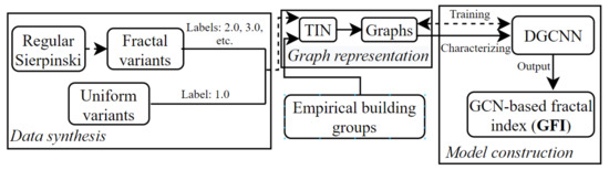
Figure 1.
Framework for characterizing complexity of building distributions.
3.2. Synthetic Fractals and Uniform Variants
The collection of training datasets generally entails either manual annotations of real patterns by individuals’ cognition [46] or automatic synthesis with algorithms [49]. Simple patterns, such as linear or grid-shaped layouts represent just one kind of a simple scenario that could be effortlessly identified by a human observer or be modeled with few geometric variables. However, it is challenging to annotate the complexity of an irregular building distribution, because of the limitations and subjectivity of human visual cognition towards complex patterns. Hence, for this work, we opted for the acquisition of training data by synthesis using algorithms. In this paper, we generate two sorts of syntheses: fractal and uniform patterns.
A fractal pattern has three aspects to unfold: morphology, uncertainty, and dimensionality [1,50]. Morphology refers to the geometrical shape that a fractal pattern exhibits. Uncertainty is here considered as the randomness in reality, while dimensionality is the degree of scales that a fractal pattern unfolds. These three components of fractals have been extensively applied to simulate natural phenomena, such as trees, terrain, and coastlines [2,51,52]. A great many regular fractal patterns have been discovered or created, such as the Vicsek fractal [53], the Koch snowflake and the Sierpinski carpet. Here, we adopt the square-based Sierpinski carpet as the fractal basis to generate fractal variants, because it is deemed as a standard pattern to measure the complexity of urban built-up areas in most urban morphology studies [8,10,29,54]. The uncertainty is triggered by a randomness mechanism under the second definition of fractals proposed by Mandelbrot [1], as it is statistical rather than geometrical. We further devised a spatial structure to locate the generated squares in regular 2D grids (see Figure 2). The degree of dimensionality towards a Sierpinski carpet is simply set as the number of recursive depths.
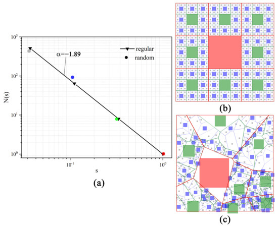
Figure 2.
(color online) The statistical relationship between the number of squares, N, and scales, s, of the Sierpinski carpet and its variants (a); a Sierpinski carpet with the degree of dimensionality 4 (b) and a randomly synthesized variant (c), where the Ns are 1, 8, 75 and 500 for the red, green, blue and grey squares, respectively.
Statistically, the fractal variants are built from the Sierpinski carpet. The construction of the Sierpinski carpet starts from a square. This square is partitioned into nine congruent sub-squares in a 3-by-3 grid, and then the central square is removed. This technique is iterated recursively on each of the remaining eight sub-squares and so forth. From the initial square, where the scale is defined to be 1, each sub-square is divided by a scaling factor of 1/3. According to the first definition of fractals, the number of squares (N) and its corresponding scales (s) have a power-law relationship described as N = s(−α) where α is the scaling factor or so-called fractal dimension. Here, as the number of squares increases eight times compared to the number of the prior scale and because the scales decrease by a factor of 1/3, the fractal dimension α is calculated as log 8/log3 ≈ 1.89. The scale is further represented as s = (1/3)c, where c is the degree of dimensionality for the complexity of the carpet. The idea of randomness suggested by the second definition of fractals is to add some random numbers to the scales (), the number of squares () and the random locations in space; meanwhile, the fractal dimension (α) should be approximately retained. In this way, the number of squares and the scales can slightly vary at each generation but still statistically follow the Sierpinski pattern. The number of squares, N, is introduced as:
where is the scale, and and are random factors resulting in some variants that deviate from the ideal (regular) scaling line (Figure 2a).
Spatially, the generated squares also entail random distributions in a 2D plane. According to the construction process of the Sierpinski carpet (see Figure 2b), the initial square is first divided into a grid with cells and then the grids cells, except the central one, are further subdivided into a children grid; this process continues recursively until the predefined dimensionality is reached. Unlike this evenly partitioning approach, for a random Sierpinski variant, the division of space in each scale is to some degree conducted at random; hence, the resulting grids and cells on the same scale levels are not congruent but irregular polygons, which we here referred to as “containers”. The centers of containers are randomly distributed within the space of their parent-containers on the higher-level scales. As an example, shown in Figure 2c, the whole space is first randomly divided into nine red containers and each of them is further recursively divided into nine green ones, each of which contains nine grey ones in the final level. The random division of space is hereby conveniently accomplished with Voronoi diagram algorithms.
Next, the synthesis of uniform variants is straightforward. A uniform distribution is a grid-like arrangement, where all building shapes are congruent squares and have an identical distance from each other. This can be easily achieved by iteratively increasing the resolution of the regular grids at different levels.
3.3. Graph Representations for Building Groups
The spatial relationships between buildings in a group are represented by a graph defined as , where V denotes the nodes for individual buildings, E refers to the links or spatial connections between neighbors, and represents a signal or feature that each node maintains. The feature can be a multi-dimensional vector, wrapping several variables that characterize the building properties. Here the feature is a two-dimensional vector where is the area of the building, and is the average distance from the node to its neighbors, that is . In this study, the graph is undirected, and the connections of building neighbors are constructed from triangulated irregular networks (TIN) (an example is shown in Figure 3). Please note though that as convolutional operations in GCN layers require self-loop connections to the nodes themselves, these also need to be added.
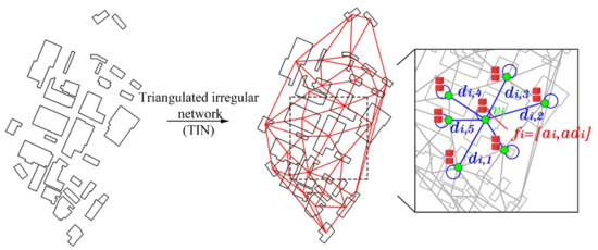
Figure 3.
(color online) Graph construction and representation for building groups: red lines are the TIN’s edges, blue lines show the distances, to the neighbors, and every two red blocks constitute a two-dimensional vector of node .
3.4. DGCNN Model
By representing building groups as graphs, their spatial features including building areas and distances can be further aggregated and represented in multiple stacked GCN layers (see Figure 4). In addition, as the aggregated spatial features implicitly exhibit the property of statistical heterogeneity, the latter can be characterized by attaching a sorting layer and a few traditional convolutional neural network layers. In our study, these deep neural networks are assembled by adopting a full-size DGCNN model.
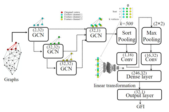
Figure 4.
(color online) The DGCNN model maps graph representations to GFI. As an example, the figure highlights four vertices–A, B, C and D–and demonstrates how the GCN and SortPooling layers extract features. The scalars in brackets demonstrate how the dimensions of neuron matrices are defined in each layer. The parameter, k, defines the number of elements taken in account during the SortPooling operations.
A DGCNN has three stages [48]: (1) stacking four GCN layers to extract local features. The aim of GCN layers is to apply convolutional operations to graphs. Like the traditional convolution neural networks (CNN), GCN also learns effective kernels to aggregate and detect localized attribute features (c.f. [43,55]). Unlike most GCN models, DGCNN organizes the four GCN layers by first stacking them one after another and taking out the results from each of them as one part of the combined results in the final GCN layer; (2) devising a SortPooling layer to sort the detected vertex features into a consistent order and to pick the first vertices before feeding them into the traditional convolutional and dense layers and (3) attaching a traditional convolution model to apply filters on the vertices’ sorted features. This final stage includes producing five sequential layers: a traditional 1-D convolutional layer, a max pooling layer, another 1-D convolutional layer, a fully connected dense layer, and an output layer. The parameter settings of the model are shown in Figure 4.
The model of DGCNN is implemented using the PyTorch backend and the Deep graph library (DGL). Moreover, the training labels of graphs are set to 1.0 for the uniform variants, and 2.0, 3.0, etc., for the fractal variants based on their dimensionality. The graph attributes of both the training and test dataset were normalized following the Z-score strategy as follows: , where is the mean value and is the standard deviation of the attributes.
3.4.1. GCN Layers
A GCN layer applies the convolutional manipulations on graphs. For a traditional CNN layer, the convolution is commonly applied to regular data structures, such as images. The features of an image are basically aggregated by a rectangular weighting scheme, a matrix, for instance, pixel by pixel. In contrast, a graph is commonly an irregular structure in which the number of neighbors of nodes is not a constant. To apply regular schemes to its features, the graph can be first represented as an adjacency matrix and then transformed to be a regular structure in the spectral domain by the basic elements of the adjacency matrix, i.e., the orthogonal bases. For a graph and its node feature matrix , where N is the number of vertices and M is the dimension of feature signals, a graph convolutional operation symbolized as “ ” is represented as follows:
where Z is the output of a GCN layer; is a nonlinear function of the frequencies of graph A with trainable parameters . is the orthogonal matrix and is its corresponding transpose. is the decomposition of X based on in the spectral domain. To extract multi-scale features, multiple GCN layers are stacked in the following manner:
where is the output of the ith GCN layer. Note, that the GCN model we used in this paper is identical to the convolutional filters proposed in [43]. By stacking multiple GCN layers, the detected features are concatenated together by the last GCN layer and further fed to a SortPooling layer.
3.4.2. The SortPooling Layer
Literally, the SortPooling layer is a pooling process toward the sorting features. The pooling layer is to reduce the spatial size of processing data in memory and the number of training parameters. For the traditional graph regression frameworks, such as the neural network for graph (NN4G) [56] and the diffusion-convolutional neural networks (DCNN) [57], the detected features are aggregated by either simple summation or averaging process, and the topological variation of the detected features between the vertices is lost. The sorting process here thus is to highlight the structural roles of vertices in the graph [42].
The inputs, i.e., a tensor where and in the work presented here, of the SortPooling layer are the concatenated vertex features from the previous GCN layer. Each row of this tensor corresponds to a detected feature descriptor of each vertex and every single column is a featured channel from the previous three GCN layers, respectively. Then, the vertex features are sorted in a lexicographically descending order: the feature tensors are firstly sorted based on the 1st channel and if some have the same values on the 1st channel, they are further sorted based on the value of the 2nd channel, and so on (see Figure 4). This algorithm has similar logic to how the vocabularies are organized in alphabetical order in dictionaries. Finally, the SortPooling layer stretches the sorting features to a vector for the subsequent traditional convolutional layers.
4. Synthetic Variants and Model Training
Two types of variants are synthesized: fractal and uniform ones. Corresponding to the dimensionality (i.e., the number of iterations) of fractals, four levels of the Sierpinski patterns labeled as 2.0, 3.0, 4.0 and 5.0 were synthesized, and the number of random variants in each level is 500. From the synthesis process shown in 3.2, it is apparent that there are around squares for a variant in level-i, for example, there are 9, 77, 589 and 4096 squares from level-2 to level-5. For the fractal patterns above level-5, there are too many squares (for example, more than 37,000 for squares in level-6) to be appropriate for building groups at the neighborhood level. Thus, any attempt to handle building groups bigger than level-5 is beyond the scope of this study. In addition, we accordingly synthesize the uniform variants whose dimensions range from to (62 variants in total and 30 duplicates for each, i.e., 62 30 = 1860 uniform variants), and labeled as 1.0 (shown in Figure 5a).
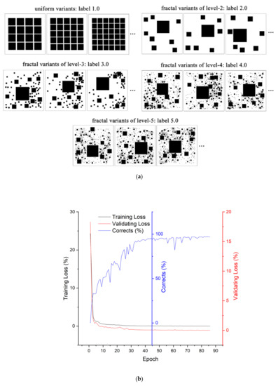
Figure 5.
(color online) Examples of synthetic variants and the process of model training: (a) the uniform synthesis labeled as 1.0 and fractal variants with the dimensionality from level-2 to level-5 labeled from 2.0 to 5.0 individually and (b) the training loss, validating loss and accuracy of the training process over each epoch.
Then, the synthetic variants of uniform and fractal patterns are combined as a training dataset and fed to the DGCNN model. The variants are shuffled randomly and divided into three parts: the training, validating, and testing data sets by a ratio of 6:2:2. In each epoch of the training process, we also estimate the training loss, validating the loss and accuracy rate of the predicted labels. Both the training and validating loss decrease rapidly and approach 0, while the correctness of the classification of fractal variant patterns increases from 1.0% to 96.5% at last. Generally, the training process terminates after a few epochs (90 epochs, in this case, shown in Figure 5b) indicating that a GFI model with highly accurate predictions is acquired.
5. Case Studies
5.1. Building Footprints in Blocks
In this study, the building footprints in London were chosen to demonstrate the performance of the proposed model. London has three zones: Greater London, the intermediate zone, and the central core zone (Table 1). To acquire the building groups, feature datasets including buildings, streets and rivers were collected from the Open Street Map website (accessed on 15 October 2020; see the download website: https://download.geofabrik.de/), a popular open-source platform allowing users to share and contribute to the crowdsourcing geo-datasets. We first generated the street blocks by aggregating all the types of street and river features and then, by the generated street blocks, we further partitioned the buildings into groups. In total, there are almost 0.48 million buildings and 24 thousand street blocks in the Greater London zone. In addition, the intermediate zone with only twenty percent of the whole area takes up almost half of the buildings and 40% of the street blocks. Considering its area, the central zone is like a reduced version of the intermediate zone, where the number of buildings and street blocks in the central zone are all about ten percent of that in the intermediate zone.

Table 1.
The statistics in The Greater London, intermediate zone and central core zone about the area, number of buildings and street blocks with their ratios relative to those of the Greater London.
The grouped buildings in London were transformed into graph representations according to Section 3.2 and their GFI values were estimated by the trained model (see results in Figure 6). In the magnified areas of interest in Figure 6 (below), the acquired GFI values are mapped to colors showing the complexity of the building groups: the greater the values are, the more complex the building groups are. In the context of London, the GFI values range from 0 to 5.90. For visualization, they are classified into six intervals with colors ranging from grey (lowest) to dark blue (highest). The GFI values of the grey blocks are set as zeros as the numbers of their buildings are less than three–the minimum number to construct a Delaunay graph. At a glance, the blocks with GFI values ranging from 0.01 to 2.5 account for the majority and distribute densely all over the three hierarchical London zones. The blocks with GFI > 2.5, however, are fewer by comparison and they are mostly located outside of the central core zone.
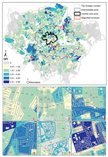
Figure 6.
(color online) The GFI distribution of building groups in the Greater London, intermediate zone and central core zone; more details are exhibited in the six magnified windows shown in the 1–6.
In addition, the spatial distribution of GFI values in London is also revealed by their descriptive statistics shown in Figure 7. Obviously, the GFI values in three zones demonstrate similar distributions with identical mean values of 1.70 and similar standard deviations. Such similarity shared between the nested zones reveals a reoccurring pattern in London: the complexity of building groups is not only more or less similar but also quite simple. Additionally, the complex building groups with GFI values greater than 4.0 are mostly in the outskirts of the central core zone; this is in line with the inspections from the spatial distribution of GFI values shown in Figure 6.
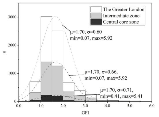
Figure 7.
Distribution of GFI values in the Greater London, intermediate zone, and central core zone.
5.2. Building Footprints in Neighborhood
For a detailed inspection of how the distribution in neighborhoods, namely in street blocks, is characterized by GFI, 34 building groups were randomly collected and listed in Figure 8. In general, the GFI values range from 0.79 to 5.65 and increase gradually as the distribution of building groups becomes more and more complex. For example, the distributions with GFI values around 1.0 are apparently simple and very similar to the grid-like pattern and those with large GFI values of approximately 5.0 demonstrate fractal-like patterns. Note, for the distributions with GFI values around 2.0, 3.0, or 4.0, namely the levels of predefined complexity there exists one largest building in terms of the area or distance compared to the remaining buildings. This matches well with the pattern that a typical Sierpinski variant exhibits: there is one single largest square while there are many others on small ones. Such a pattern within a small range could be treated as a mono structure and it could be recursively combined or mixed progressively to form more complex wholes until another big building on a higher scale shows up. This gradual change in building distributions can also be observed in the examples shown in Figure 8.
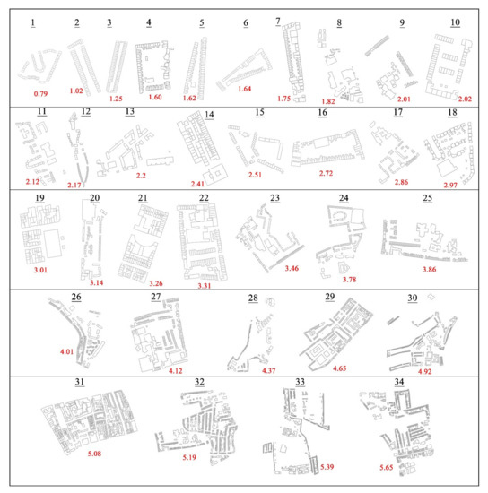
Figure 8.
(color online) Building footprints in neighborhood labeled by GFI: from the simple uniforms to complex fractals.
To further compare how GFI values characterize the complexity of building groups, two descriptors are also calculated including the number of buildings, the density of built-up area (the ratio between the areas of buildings and the minimum bounding boxing), and the classical complexity indicators (i.e., the fractal dimension (FD), ht-indices and CRG indices for the areas (ht-A and CRG-D) and distance of building groups (ht-A and CRG-D)) (see Table 2). Notably, none of the mentioned descriptors or indicators can characterize the complexity of building distributions. The number of buildings seems to reflect well the increase of the complexity, but it is a necessary rather than a sufficient condition, namely that a complex distribution does not require many buildings and vice versa. The density of built-up area also makes no difference to the morphological complexity. For example, the densities of No. 3 and 31 are almost equal, but it is obvious that No. 31 is much more complex than No. 3.
Table 2.
The fractal indices of the neighborhoods in Figure 7: the GFI, ht, CRG, FD of area and distance (‘-A’ is ‘-area’ and ‘-D’ is ‘-distance’ for short).
Moreover, the CRG indices (CRG-A/D) are more sensitive than the ht-indices (ht-A/D). As the distributions turn more and more complex, the CRG-A/D increase, while the ht-A/D do not change accordingly. Especially the change in CRG-A is more prominent than that of CRG-D. The CRG-D even drops to 0 although the pattern of its counterpart is complex (Figure 9). However, neither the CRG nor ht-indices could well quantify how the complex building patterns evolve. This is simply illustrated by two pairs of building distributions, No. 6–No. 29 and No. 11–No. 29, wherein each pair has either similar CRG or ht-indices but significantly different structural patterns. In addition, the apparent outliers of CRG values (the bold texts in Table 2 and marked by red circles in Figure 9) seem too sensitive to identify the corresponding patterns. Lastly, the FD is also not capable to characterize the complexity in a good manner. Comparing No. 3 and No. 31, for example, both have similar FD values as well as built-up densities, but their degrees of complexity are strikingly different.
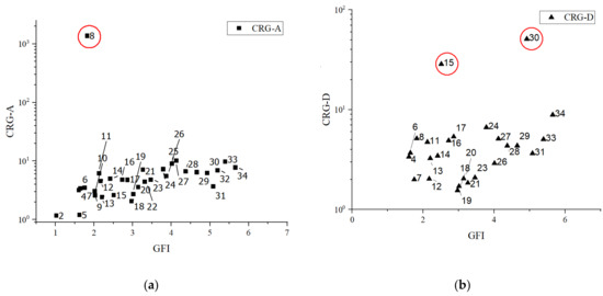
Figure 9.
(color online) Distributions between GFI and CRG-A (a), CRG-D (b) of the 34 examples shown in Table 2; the outliers of CRG values are marked by the red circles.
6. Discussion
A novel graph-based fractality index (GFI) to characterize the building distribution’s complexity is proposed. It is based on the second definition of fractals and a GCN-based deep learning model–DGCNN. To test the new index, building footprints of street blocks over three hierarchically nested London areas were used: The Greater London, the intermediate zone and the central core zone. According to the statistical distribution of GFI values, the complexities of most building distributions in these areas are quite small, indicating simple structures. This may be somewhat surprising, as London has been claimed as a complex system or an organic whole [14]. However, the index shows that it still consists of many simple and well-organized structures, probably due to active and deliberate planning during the expansion of the urban development. Nevertheless, the standard deviations of GFI in the three areas increase from the big Greater London area towards the intermediate central core zone (cf. Figure 7). In other words, the fluctuation of GFI mostly demonstrates how diverse the building distributions are within each zone, from a low diversity in the Greater London zone to high diversity in the intermediate zone. This suggests an interesting spatial evolving pattern of buildings from the central area in London to the periphery, i.e., gradually and naturally including changes and replacements of buildings in the area through time, whereas the outskirts probably have been developed more suddenly through simultaneous construction of larger areas at a coarser scale. In this respect, the morphological complexity quantified in terms of the GFI values can also show the diversity of urban development on city scales and may further demonstrate the extent of human movement in socio-economical terms.
GFI has a multi-fold advantage over previous fractal metrics FD, ht-index, and CRG in characterizing both spatial and statistical distribution of buildings. At high building densities, the results show that the FD cannot differentiate how complex the building distribution is in space. A high-density distribution could have two totally contrasting patterns: a very regular grid-like pattern or a highly disordered one, where both FDs are approaching the value of 2.0. This happens because it measures the extent of space-filling, such as the number of boxes, rather than the spatial distribution patterns of targets per se. This finding also agrees with the report by Thomas, Frankhauser, and Biernacki [54] that FD is exponentially correlated with density. The ht-index and CRG on the other hand turn to the distribution of targets, and in this sense, these indices complement the FD. Yet, due to the essence of statistical distribution, the ht-index and CRG cannot quantify the complexity of building distributions in terms of areas and distances, respectively. The examples shown in Table 2 suggest that, either for the area or distance, similar values in terms of ht-index and CRG index do not necessarily reveal a similar pattern of building distributions. The ht-index, for example, works with discrete integers so that the gradual changes cannot be well represented. Additionally, note that the CRG occasionally behaves extremely differently, generating peculiar outliers (shown in Figure 9). To be specific, these outliers appear when their corresponding ht-index equals 2. By reviewing its definition [31], it is therefore suggested that, under this circumstance, the CRG should equal 1 instead of the first average attribute values. The proposed GFI takes up both the spatial and statistical distribution of a building group to characterize its complexity, where the distribution visually matches the given GFI (Figure 8 and Table 2). As the basic idea behind the proposed framework is built upon characterizing both the spatial and the statistical distribution, by the second and third fractal definition, respectively, the GFI thus complements the FD, ht-index and CRG, and fulfills a descriptive ability toward spatial complexity, in general. In addition, the number of buildings in the neighborhood demonstrates a seemly positive relationship with the GFI values (see Table 2), but a further examination based on the whole dataset of the neighborhood blocks in London shows that the number of buildings is not strongly positive-correlated with the GFI value. For the groups with a larger number of buildings, their GFI values are basically greater but not vice versa. In this regard, the groups with higher GFI values can have either fewer or more buildings but all demonstrate complex spatial characteristics including the number of buildings.
The framework proposed in this work is, to our knowledge, the first attempt to take the advantage of deep learning models and fractal theories to solve the problem of complexity measurement. The complex phenomenon of building distribution (i.e., spatially and statistically) can be represented by graphs and learned by GCN-based deep learning models. Building distributions basically have three features: attributes, spatial distributions, and the relationships or interactions between neighbors. As shown in the results, it is a difficult task to build a linear model, such as the ht-index, CRG and FD, to include all these factors at the same. Hence, by using the strength of the GCN models, effective non-linear data can be represented by numerous computational neurons. Deep learning has been criticized for its inexplicability and is treated as a “black box”. However, essentially it is a non-linear function integrated with multiple linear regression equations layer by layer [35], where its hidden neurons are the variables of the regression functions and the parameters are the learned coefficients. The structurally organized neurons also maintain a good learning ability for the spatial features across different hierarchical scales. This idea is in line with the operation of the graph Fourier transforms (i.e., the graph signals are decomposed into hierarchical ones with different frequencies) implemented by the GCN layers. Introduced by the DCGNN model, the hierarchically organized GCN layers and the sorting layer along with the traditional convolutional layers also well address the shortcoming that previous GCN models cannot differentiate heterogeneous datasets [46,48], such as building distributions.
The introduced synthetic fractal variants by fractal theories also provide the possibility of unlimited samples in the training process. Under the second definition of fractals, it has been shown that it is possible to synthesize fractal variants with labels according to their fractal complexity and that the trained deep learning model performs well to quantify the complexity of building distributions. To be noticed, in the context of different scales, the corresponding polygonal feature groups should also be adapted. For example, if all the building footprints are included to indicate one single city, the GFI would be large and there is no big difference between cities. It is obvious that the buildings are diverse in terms of areas and distance in any city at the urban scale. Instead of the building features, however, the street blocks may be a better candidate. Meanwhile, as the synthetic dataset is generated by a purely mathematical concept of fractal patterns, the Sierpinski carpet, for example, the model is general enough so that it is independent of any specific geographical scenarios, which further assures the ability of model generalization to a large extent. Such a strategy reduces, or basically avoids, the dilemmas concerning both the difficulty of data acquirement and the ability of model generalizations for most data-driven models, which have been criticized and thought of as a bottleneck [58]. This is in line with the suggestion that it is worthy to bridge theoretical and mathematical generated patterns with data-driven science, especially under the current fourth GIScience paradigm [59].
From a practical urban planning point of view, the method as such, as well as a future easy-to-use tool can, for example, be used to see how different existing environments connect with people’s wellbeing and health [60,61], or if some patterns have implications for traffic flows, fire risks and blue-light emergency services [62,63]. It has the potential to aid future planning scenarios using what-if modeling approaches and VR [64]. Those potential applications with fruitful or high-dimensional properties can also be nominated as aspatial signals in the GFI model to indicate the complexity of discovered patterns as well as their better understanding. Under the 3D-urban context, for example, combined with human component properties, such as population densities, building stories and land use, GFI may further facilitate to outline the patterns of social-economic development. A recent Swedish study by Amcoff [65,66], e.g., points out that the 50-year-old strategy of mixed-income housing in a neighborhood has yielded very little in terms of combatting segregation. Instead, the urban form and the connectivity between the urban parts seem to be better indicators of segregation. The GFI approach, hence, may serve as a valuable tool to describe such patterns. GFI in addition to its computational framework also opens up new possibilities to measure complexity in other scenarios, especially towards spatial targets, such as land cover and urban climate, or even medical-related content, such as the recognition of tumors. Moreover, diverse applications may entail other interesting features and even proper fractal patterns, which may be inspirational drivers to explore more potentials of the combination of fractals and data-driven science and to establish a new kind of complex science in the future.
7. Conclusions
In this study, a graph-based fractality index, GFI, based on a hybrid of fractal theories and deep learning techniques is proposed to value or measure the complexity of spatial features, such as building footprints in a given area. The tests on building footprints have shown the index’s feasibility to differentiate the complex patterns and also demonstrate the shortcomings of previous indices, such as fractal dimension, the ht-index and CRG. Synthesizing fractal variants in a systematic manner based on the second definition of fractals also seems to assure that the trained deep learning is objective and not affected by potential biases in empirically selected training datasets. By using fractal concepts, spatial complexity can be estimated and provides a benchmark to understand and compare different areal settings. In this context, the question of spatial complexity can be shifted to that of spatial fractality. The use of GFI to study the spatial complexity in our living environment has the potential to evaluate, maintain, and refine sustainable and resilient human development. Future exploration of the hybrid of different fractal patterns and machine learning algorithms in diverse contexts would be a promising topic for both the academic and industry and is of interest in our forthcoming work.
Author Contributions
Conceptualization, Lei Ma, Stefan Seipel, Sven Anders Brandt and Ding Ma; methodology, Lei Ma, Stefan Seipel, Sven Anders Brandt and Ding Ma; software, Lei Ma; data curation, Lei Ma; writing—original draft preparation, Lei Ma; writing—review and editing, Lei Ma, Stefan Seipel, Sven Anders Brandt and Ding Ma; visualization, Lei Ma; supervision, Stefan Seipel, Sven Anders Brandt and Ding Ma. All authors have read and agreed to the published version of the manuscript.
Funding
Funding provided by University of Gävle.
Acknowledgments
We thank the anonymous reviewers for helpful comments and constructive advice on earlier vesions of the manuscript.
Conflicts of Interest
The authors declare no conflict of interest.
References
- Mandelbrot, B.B. The Fractal Geometry of Nature; W. H. Freeman and Company: New York, NY, USA, 1982. [Google Scholar]
- Mandelbrot, B.B. How Long Is the Coast of Britain? Statistical Self-Similarity and Fractional Dimension. Science 1967, 156, 636–638. [Google Scholar] [CrossRef] [PubMed] [Green Version]
- Lauwerier, H. Fractals: Endlessly Repeated Geometrical Figures; Gill-Hoffstädt, S., Translator; Princeton University Press: Princeton, NJ, USA, 1991. [Google Scholar]
- Jiang, B.; Yin, J. Ht-Index for Quantifying the Fractal or Scaling Structure of Geographic Features. Ann. Assoc. Am. Geogr. 2013, 104, 530–540. [Google Scholar] [CrossRef]
- Jiang, B.; Brandt, S.A. A Fractal Perspective on Scale in Geography. ISPRS Int. J. Geo. Inf. 2016, 5, 95. [Google Scholar] [CrossRef] [Green Version]
- Jiang, B.; Ma, D. How Complex Is a Fractal? Head/tail Breaks and Fractional Hierarchy. J. Geovisualization Spat. Anal. 2018, 2, 6. [Google Scholar] [CrossRef] [Green Version]
- Batty, M.; Longley, P.A. Fractal Cities: A Geometry of Form and Function; Academic Press Inc.: San Diego, CA, USA, 1994. [Google Scholar]
- Tannier, C.; Thomas, I.; Vuidel, G.; Frankhauser, P. A Fractal Approach to Identifying Urban Boundaries. Geogr. Anal. 2011, 43, 211–227. [Google Scholar] [CrossRef]
- Tannier, C.; Thomas, I. Defining and characterizing urban boundaries: A fractal analysis of theoretical cities and Belgian cities. Comput. Environ. Urban Syst. 2013, 41, 234–248. [Google Scholar] [CrossRef]
- Thomas, I.; Frankhauser, P. Fractal Dimensions of the Built-up Footprint: Buildings versus Roads. Fractal Evidence from Antwerp (Belgium). Environ. Plan. B Plan. Des. 2013, 40, 310–329. [Google Scholar] [CrossRef]
- Rootzén, H.; Segers, J.; Wadsworth, J.L. Multivariate generalized Pareto distributions: Parametrizations, representations, and properties. J. Multivar. Anal. 2018, 165, 117–131. [Google Scholar] [CrossRef] [Green Version]
- Liu, Z.; Zhou, J. Introduction to Graph Neural Networks. Synth. Lect. Artif. Intell. Mach. Learn. 2020, 14, 1–127. [Google Scholar] [CrossRef]
- Batty, M. Inventing Future Cities; Batty, M., Ed.; The MIT Press: Cambridge, MA, USA, 2019. [Google Scholar] [CrossRef]
- Ma, D.; Osaragi, T.; Oki, T.; Jiang, B. Exploring the heterogeneity of human urban movements using geo-tagged tweets. Int. J. Geogr. Inf. Sci. 2020, 34, 2475–2496. [Google Scholar] [CrossRef]
- D’Acci, L. Mathematics of Urban Morphology; Luca, D., Ed.; Birkhäuser: Basel, Switzerland, 2019. [Google Scholar]
- Hillier, B.; Hanson, J. The Social Logic of Space; Cambridge University Press: Cambridge, UK; New York, NY, USA, 1984. [Google Scholar] [CrossRef]
- Zhang, X.; Stoter, J.; Ai, T.; Kraak, M.J.; Molenaar, M. Automated evaluation of building alignments in generalized maps. Int. J. Geogr. Inf. Sci. 2013, 27, 1550–1571. [Google Scholar] [CrossRef]
- Zhang, X.; Ai, T.; Stoter, J. Characterization and detection of building patterns in cartographic data: Two algorithms. In Advances in Spatial Data Handling and GIS; Springer: Berlin/Heidelberg, Germany, 2012; pp. 93–107. [Google Scholar]
- Zhao, R.; Ai, T.; Yu, W.; He, Y.; Shen, Y. Recognition of building group patterns using graph convolutional network. Cartogr. Geogr. Inf. Sci. 2020, 47, 400–417. [Google Scholar] [CrossRef]
- He, X.; Zhang, X.; Xin, Q. Recognition of building group patterns in topographic maps based on graph partitioning and random forest. ISPRS J. Photogramm. Remote Sens. 2018, 136, 26–40. [Google Scholar] [CrossRef]
- Du, S.; Zhang, F.; Zhang, X. Semantic classification of urban buildings combining VHR image and GIS data: An improved random forest approach. ISPRS J. Photogramm. Remote Sens. 2015, 105, 107–119. [Google Scholar] [CrossRef]
- Niu, N.; Liu, X.; Jin, H.; Ye, X.; Liu, Y.; Li, X.; Chen, Y.; Li, S. Integrating multi-source big data to infer building functions. Int. J. Geogr. Inf. Sci. 2017, 31, 1871–1890. [Google Scholar] [CrossRef]
- Lüscher, P.; Weibel, R.; Burghardt, D. Integrating ontological modelling and Bayesian inference for pattern classification in topographic vector data. Comput. Environ. Urban Syst. 2009, 33, 363–374. [Google Scholar] [CrossRef] [Green Version]
- Li, Z.; Yan, H.; Ai, T.; Chen, J. Automated building generalization based on urban morphology and Gestalt theory. Int. J. Geogr. Inf. Sci. 2004, 18, 513–534. [Google Scholar] [CrossRef]
- Batty, M.; Kim, K.S. Form Follows Function: Reformulating Urban Population Density Functions. Urban Stud. 1992, 29, 1043–1069. [Google Scholar] [CrossRef]
- Thomas, I.; Frankhauser, P.; De Keersmaecker, M.-L. Fractal dimension versus density of built-up surfaces in the periphery of Brussels. Pap. Reg. Sci. 2007, 86, 287–308. [Google Scholar] [CrossRef]
- Sémécurbe, F.; Tannier, C.; Roux, S.G. Applying two fractal methods to characterise the local and global deviations from scale-invariance of built patterns throughout mainland France. J. Geogr. Syst. 2019, 21, 271–293. [Google Scholar] [CrossRef] [Green Version]
- Lagarias, A.; Prastacos, P. Comparing the urban form of South European cities using fractal dimensions. Environ. Plan. B Urban Anal. City Sci. 2018, 47, 1149–1166. [Google Scholar] [CrossRef]
- Thomas, I.; Frankhauser, P.; Badariotti, D. Comparing the fractality of European urban neighbourhoods: Do national contexts matter? J. Geogr. Syst. 2010, 14, 189–208. [Google Scholar] [CrossRef]
- Gao, P.; Liu, Z.; Xie, M.; Tian, K.; Liu, G. CRG Index: A More Sensitive Ht-Index for Enabling Dynamic Views of Geographic. Features Prof. Geogr. 2015, 68, 533–545. [Google Scholar] [CrossRef]
- Gao, P.; Zhao, L.; Kun, T.; Gang, L. Characterizing traffific conditions from the perspective of spatial-temporal heterogeneity. ISPRS Int. J. Geo. Inf. 2016, 5, 34. [Google Scholar] [CrossRef] [Green Version]
- Gao, P.; Liu, Z.; Liu, G.; Zhao, H.; Xie, X. Unified metrics for characterizing the fractal nature of geographic features. Ann. Am. Assoc. Geogr. 2017, 107, 1315–1331. [Google Scholar] [CrossRef]
- Jiang, B. Head/Tail Breaks: A New Classification Scheme for Data with a Heavy-Tailed Distribution. Prof. Geogr. 2013, 65, 482–494. [Google Scholar] [CrossRef]
- Ren, Z.; Jiang, B.; Seipel, S. Capturing and Characterizing Human Activities Using Building Locations in America. ISPRS Int. J. Geo. Inf. 2019, 8, 200. [Google Scholar] [CrossRef] [Green Version]
- Xu, K.; Hu, W.; Leskovec, J.; Jegelka, S. How powerful are graph neural networks? In Proceedings of the 7th International Conference on Learning Representations, ICLR 2019, New Orleans, LA, USA, 6–9 May 2019; pp. 1–17. [Google Scholar]
- Hu, W.; Yan, L.; Liu, K.; Wang, H. A Short-term Traffic Flow Forecasting Method Based on the Hybrid PSO-SVR. Neural Process. Lett. 2015, 43, 155–172. [Google Scholar] [CrossRef]
- Li, Y.; Yu, R.; Shahabi, C.; Liu, Y. Diffusion Convolutional Recurrent Neural Network. In International Conference on Learning Representations; University of California: Oakland, CA, USA, 2018; Volume 1090, pp. 1–15. [Google Scholar]
- Jin, G.; Cui, Y.; Zeng, L.; Tang, H.; Feng, Y.; Huang, J. Urban ride-hailing demand prediction with multiple spatio-temporal information fusion network. Transp. Res. Part C Emerg. Technol. 2020, 117, 102665. [Google Scholar] [CrossRef]
- Yi, X.; Zhang, J.; Wang, Z.; Li, T.; Zheng, Y. Deep Distributed Fusion Network for Air Quality Prediction. In Proceedings of the KDD ’18: 24th ACM SIGKDD International Conference on Knowledge Discovery & Data Mining, New York, NY, USA, 19–23 August 2018. [Google Scholar] [CrossRef]
- Yu, L.; Jiao, C.; Xin, H.; Wang, Y.; Wang, K. Prediction on Housing Price Based on Deep Learning. Int. J. Comput. Inf. Eng. 2018, 12, 90–99. [Google Scholar] [CrossRef]
- Yildirimoglu, M.; Kim, J. Identification of communities in urban mobility networks using multi-layer graphs of network traffic. Transp. Res. Part C Emerg. Technol. 2018, 89, 254–267. [Google Scholar] [CrossRef]
- Niepert, M.; Ahmed, M.; Kutzkov, K. Learning convolutional neural networks for graphs. In International Conference on Machine Learning; ICML 2016 4; PMLR: New York, NY, USA, 2016; pp. 2958–2967. [Google Scholar]
- Kipf, T.N.; Welling, M. Semi-supervised classification with graph convolutional networks. In Proceedings of the 5th International Conference on Learning Representations, ICLR 2017, Toulon, France, 24–26 April 2017. [Google Scholar] [CrossRef]
- Zheng, C.; Fan, X.; Wang, C.; Qi, J. GMAN: A Graph Multi-Attention Network for Traffic Prediction. Proc. Conf. AAAI Artif. Intell. 2020, 34, 1234–1241. [Google Scholar] [CrossRef]
- Wu, Y.; Lian, D.; Xu, Y.; Wu, L.; Chen, E. Graph Convolutional Networks with Markov Random Field Reasoning for Social Spammer Detection. Proc. Conf. AAAI Artif. Intell. 2020, 34, 1054–1061. [Google Scholar] [CrossRef]
- Yan, X.; Ai, T.; Yang, M.; Yin, H. A graph convolutional neural network for classification of building patterns using spatial vector data. ISPRS J. Photogramm. Remote Sens. 2019, 150, 259–273. [Google Scholar] [CrossRef]
- Yan, X.; Ai, T.; Yang, M.; Tong, X. Graph convolutional autoencoder model for the shape coding and cognition of buildings in maps. Int. J. Geogr. Inf. Sci. 2020, 35, 490–512. [Google Scholar] [CrossRef]
- Zhang, M.; Cui, Z.; Neumann, M.; Chen, Y. An end-to-end deep learning architecture for graph classification. In Proceedings of the Thirty-Second AAAI Conference on Artificial Intelligence, New Orleans, LA, USA, 2–7 February 2018; pp. 4438–4445. [Google Scholar]
- Sankaranarayanan, S.; Balaji, Y.; Jain, A.; Lim, S.N.; Chellappa, R. Learning from Synthetic Data: Addressing Domain Shift for Semantic Segmentation. In Proceedings of the IEEE Computer Society Conference on Computer Vision and Pattern Recognition, San Juan, PR, USA, 17–19 June 1997; pp. 3752–3761. [Google Scholar] [CrossRef] [Green Version]
- Mandelbrot, B.B. Fractals: Form, Chance and Dimension; W.H. Freeman and Company: New York, NY, USA, 1977. [Google Scholar]
- Van Pabst, L.v.L.; Jense, H. Dynamic Terrain Generation Based on Multifractal Techniques. In High Performance Computing for Computer Graphics and Visualisation; Springer: New York, NY, USA, 1996; pp. 186–203. [Google Scholar] [CrossRef]
- Re, A.D.L.; Abad, F.; Camahort, E.; Juan, M.C. Tools for Procedural Generation of Plants in Virtual Scenes. In Lecture Notes in Computer Science; Including Subseries Lecture Notes in Artificial Intelligence and Lecture Notes in Bioinformatics 5545 LNCS (PART 2); Springer: Berlin/Heidelberg, Germany, 2009; pp. 801–810. [Google Scholar]
- Vicsek, T.; Gould, H. Fractal Growth Phenomena. Comput. Phys. 1989, 3, 108. [Google Scholar] [CrossRef]
- Thomas, I.; Frankhauser, P.; Biernacki, C. The morphology of built-up landscapes in Wallonia (Belgium): A classification using fractal indices. Landsc. Urban Plan. 2008, 84, 99–115. [Google Scholar] [CrossRef]
- Defferrard, M.; Bresson, X.; Vandergheynst, P. Convolutional Neural Networks on Graphs with Fast Localized Spectral Filtering. Adv. Neural Inf. Process. Syst. 2016, 59, 3844–3852. [Google Scholar]
- Micheli, A. Neural Network for Graphs: A Contextual Constructive Approach. IEEE Trans. Neural Netw. 2009, 20, 498–511. [Google Scholar] [CrossRef]
- Atwood, J.; Towsley, D. Diffusion-convolutional neural networks. Adv. Neural Inf. Process. Syst. 2016, 29. Available online: https://cpb-us-w2.wpmucdn.com/sites.coecis.cornell.edu/dist/9/287/files/2019/08/Towsley-6-6212-diffusion-convolutional-neural-networks.pdf (accessed on 10 February 2022).
- Heaven, D. Why deep-learning AIs are so easy to fool. Nature 2019, 574, 163–166. [Google Scholar] [CrossRef] [PubMed]
- Gahegan, M. Fourth paradigm GIScience? Prospects for automated discovery and explanation from data. Int. J. Geogr. Inf. Sci. 2019, 34, 1–21. [Google Scholar] [CrossRef] [Green Version]
- Hajrasoulih, A.; del Rio, V.; Francis, J.; Edmondson, J. Urban form and mental wellbeing: Scoping a theoretical framework for action. J. Urban Des. Ment. Health 2018, 5. Available online: https://www.urbandesignmentalhealth.com/journal-5---urban-form-and-mental-wellbeing.html (accessed on 10 February 2022).
- McCormack, G.R.; Cabaj, J.; Orpana, H.; Lukic, R.; Blackstaffe, A.; Goopy, S.; Hagel, B.; Keough, N.; Martinson, R.; Chapman, J.; et al. Evidence synthesis A scoping review on the relations between urban form and health: A focus on Canadian quantitative evidence. Health Promot. Chronic Dis. Prev. Can. 2019, 39, 187–200. [Google Scholar] [CrossRef] [PubMed]
- Trowbridge, M.J.; Gurka, M.J.; O’Connor, R.E. Urban Sprawl and Delayed Ambulance Arrival in the U.S. Am. J. Prev. Med. 2009, 37, 428–432. [Google Scholar] [CrossRef] [PubMed]
- Kumar, V.; Bandyopadhyay, S.; Ramamritham, K.; Jana, A. Pinch analysis to reduce fire susceptibility by redeveloping urban built forms. Clean Technol. Environ. Policy 2020, 22, 1531–1546. [Google Scholar] [CrossRef]
- Haifler, T.Y.; Fisher-Gewirtzman, D. Urban Wellbeing, As Influenced by Densification Rates and Building Typologies—A Virtual Reality Experiment. In Anthropocene, Design in the Age of Humans, Proceedings of the 25th CAADRIA Conference, Bangkok, Thailand, 5–6 August 2020; Chulalongkorn University: Bangkok, Thailand, 2020; pp. 661–670. [Google Scholar]
- Amcoff, J. Ny studie om segregation: Urban form kan vara viktigare än bostadsblandning. Plan Tidskr. För Samhällsplanering 2022, 1–2, 64–69. (In Swedish) [Google Scholar]
- Amcoff, J. Searching for new ways to achieve mixed neighbourhoods. Cities 2022, 121, 103496. [Google Scholar] [CrossRef]
Publisher’s Note: MDPI stays neutral with regard to jurisdictional claims in published maps and institutional affiliations. |
© 2022 by the authors. Licensee MDPI, Basel, Switzerland. This article is an open access article distributed under the terms and conditions of the Creative Commons Attribution (CC BY) license (https://creativecommons.org/licenses/by/4.0/).