A Robustness Study for the Extraction of Watertight Volumetric Models from Boundary Representation Data

Abstract

Geometrically induced topology plays a major role in applications such as simulations, navigation, spatial or spatio-temporal analysis and many more. This article computes geometrically induced topology useful for such applications and extends previous results by presenting the unpublished used algorithms to find inner disjoint $(d+1)$-dimensional simplicial complexes from a set of intersecting d-dimensional simplicial complexes which partly shape their B-Reps (Boundary Representations). CityGML has been chosen as the input data format for evaluation purposes. In this case, the input data consist of planar segment complexes whose triangulated polygons serve as the set of input triangle complexes for the computation of the tetrahedral model. The creation of the volumetric model and the computation of its geometrically induced topology is partly parallelized by decomposing the input data into smaller pices. A robustness analysis of the implementations is given by varying the angular precision and the positional precision of the epsilon heuristic inaccuracy model. The results are analysed spatially and topologically, summarised and presented. It turns out that one can extract most, but not all, volumes and that the numerical issues of computational geometry produce failures as well as a variety of outcomes.

1. Introduction

B-Reps (Boundary Representations) of geometric data such as city models are useful for retrieving the topological relationships between entities such as buildings and infrastructure elements. Ideally, they are watertight in the sense that volumes bounded by surfaces are modelled in a way that all planar border surfaces form a non-overlapping cover. A widely used data format for city models is CityGML [1], which is a B-Rep model. Complex volumes or solids are represented by a set of planar polygons which are supposed to form a watertight hull. The polygons themselves are also B-Reps to represent planar surfaces.

To compute the geometrically induced topology of this type of data is not a trivial task. In [2], it was found that such data often contains various types of topological inconsistencies, in the sense that elements have intersections which are not referenced explicitly. For this reason, data of this kind need a rendering to topologically consistent models. If the volumetric model is topologically consistent, then simulations relying on the topology of the model will capture flows of substances such as air, water, heat, pollutants, etc., through the correct elements because the correct connectivity relationships are known.

The article [3] presents a method for producing solid models from B-Rep models together with the geometrically induced topology represented as a graph. The approach there is to find inner disjoint $(d+1)$-dimensional simplicial complexes from a set of intersecting d-dimensional simplicial complexes which partly shape their B-Reps, and to triangulate these in order to create tetrahedral volume models. The overlay computation of these tetrahedral volume models in order to produce a topologically consistent model was not needed in [3], as only the volume measure was of interest. However, the geometrically induced topology is represented as a Property Graph Model using certain relation types. The Property Graph Model in turn can be used for topological queries without recalculating each intersection on demand with the help of some spatial or spatio-temporal access methods. The input data have been decomposed into different simplicial sub-complexes in order to test different kinds of parallelisations. Parallelisation is a major need to process big geo-spatial data efficiently. Three types of decompositions of the CityGML input data were tested by the definition of grouping tags. Each type of decomposition results in a number of different sets of open volumes, one set per decomposition or thread of the parallelisation. Those sets of disjoint open volumes can intersect each other. The quality of the output depends on the floating point arithmetic, the precision model and the decomposition of larger pieces into disjoint pieces, which has been performed for parallelization purposes. In other words, rounding errors, or said otherwise, uncertainty in the geometry, and the method of the decomposition can influence the global topology on which some application may rely.

The aim of this article is (a) to present the remaining algorithms to compute topologically consistent volumetric models in addition to [3], (b) to analyse the robustness of the algorithms by variation defining parameters for the equality of angles and lengths and (c) to study the speed-up and the parallelization impact on the results by using different decomposition types of input entities into smaller pieces.

The following Section 2 gives an overview of the state-of-the-art in research in related work. Section 3, on Methodology, introduces the algorithms to find B-Reps. Section 4 presents the experiments, and Section 5 discusses the findings in the context of their meaning for simulations on topologically inconsistent data.

2. Related Work

This article is a contribution to topological methods in geographical information systems (GIS) by studying the rendering method of topologically inconsistent input data from [3] with respect to its sensitivity to certain uncertainty parameters.

Already in [4], we find simplicial complexes as data structures for managing 3D/4D topological information in GIS. A theoretic foundation for topological databases for applications in geographic science or systems was laid out in [5], which relies on the mathematical result that partially ordered sets correspond to a certain large class of finite topological spaces [6]. Practically, this was implemented in [7], where the focus is on the management of topology in GIS. The review article [8] gives a more in-depth overview of applications of topology in this field of research.

Recently, it was found how to enable topology management systems to allow for a distributed implementation of simulations on topological models in GIS [9,10]. This is based on a method to obtain volumetric models from topologically inconsistent data [3]. This is a necessary step, as the widely spread format CityGML [1] contains various types of topological inconsistencies [2,11]. Notice that the literature contains various differing notions of topological consistency, cf., e.g., [12,13,14]. However, to quote from [2]:

In [15], the most common geometric and semantic errors in CityGML data are analysed. They find that the most common topological errors are that polygons are not properly oriented, and that geometries are not properly “snapped”. From what is stated there, one can see that our approach is, on the one hand, a further differentiation of that error type, and, on the other hand (unlike loc. cit.), we do not require a building to consist of solids only, as long as the polygons intersect in common boundary elements, e.g., balconies, porches, and shelters often have geometries which do not form a shell, i.e., are non-closed surfaces.

Already, Refs. [16,17] deal with finding and automatically repairing inconsistencies in CityGML data. As healing methods rely on geometrical operations which depend on rounding errors, this is an issue which deserves attention. In particular, it is of interest whether a method is robust or sensitive to variations in parameters. Such a robustness analysis can be found, e.g., in planning optimal road alignments [18]. Uncertainty or sensitivity analysis leads to tools for GIS-based model implementation [19]. As geometric operations are fundamental for GIS, robustness considerations can be found already in [20]. A first study of a method of transforming a B-Rep of a solid model into a tetrahedral space partition using rounded integer values was presented in [21], where it was found that the achievable accuracy is sufficient for the civil engineering industry. Finally, we mention error propagation using Monte Carlo methods in GIS that can be found, e.g., in [22], although we use a different method of analysis in this article.

3. Methodology

3.1. Epsilon Heuristic

The use of an epsilon heuristic is a common and straight forward inaccuracy model to use for imprecise data. Five different scaling factors need to be chosen in addition to one fixed value as the basic constant $\alpha$. The basic constant $\alpha$ has to be set to ${10}^{-n}$ with n being a desired integer number and $n>0$. So, there is one precision parameter $\alpha$ which scales all precision types and five different factors for each precision type:

1.

Base precision value $\alpha$

as base value for all the different precision types;

2.

Positional precision $ϵ=\alpha {ϵ}^{\prime }$

with factor ${ϵ}^{\prime }$ for distance, length, area and volume comparison;

3.

Positional line precision $\epsilon =\alpha {\epsilon }^{\prime }$

with factor ${\epsilon }^{\prime }$ for point- or line-on-line comparison;

4.

Positional plane precision $\sigma =\alpha {\sigma }^{\prime }$

with factor ${\sigma }^{\prime }$ for point-, line- or plane-in-plane comparison;

5.

Angular precision $\zeta =\alpha {\zeta }^{\prime }$

with factor ${\zeta }^{\prime }$ for cosine comparison;

6.

Skew precision $\lambda =\alpha {\lambda }^{\prime }$

with factor ${\lambda }^{\prime }$ for the skew comparison of two lines.

Smaller values of the positional precision $ϵ$ reduce the buffers around points, which leads to less point equality as well as smaller lengths of segments, areas of triangles and volumes of tetrahedra. Smaller values of the positional line precision $\epsilon$ reduce the buffer around lines, which leads to fewer contains and intersects identifications of a line with points and lines. Smaller values of the positional plane precision $\sigma$ lead to fewer contains and intersects identifications of a plane with lines and points. Smaller values of the angular precision $\zeta$ lead to thinner angles. This in turn leads to fewer collinear, fewer parallel and fewer orthogonal identifications of planes and lines. Smaller values of the skew precision $\lambda$ lead to fewer skew identifications when comparing two lines.

3.2. Geometrically Induced Topology

According to [2], a spatial model consisting of points, open segments and open polygons is topologically consistent if all objects are pairwise disjoint. Otherwise, it is topologically inconsistent. Consequently, if a model is topologically inconsistent, then the existing overlaps between objects are not captured in the topological model and therefore appear to be non-existent. This notion of topological consistency differs from previous definitions in the literature in that it relates geometry and topology in a meaningful way. In fact, through this, a comparison between the explicit topology of the model and the topology induced by geometry now becomes possible.

The models considered in this article are mostly simplicial complexes, i.e., their constituting objects are simplices. The textbook by Hatcher [23] contains more information about these structures. The topology of a finite simplicial complex can be captured explicitly by modelling the boundary relationships between a simplex and its bounding simplices. This gives the so-called face poset, a partially ordered set whose elements are the k-dimensional simplices for any $k\ge 0$ called faces, and the partial order relation is the inclusion of faces. According to [6], a finite partially ordered set is a certain topological space known as a so-called $T_0$-space, and vice versa every finite $T_0$-set a partially ordered set.

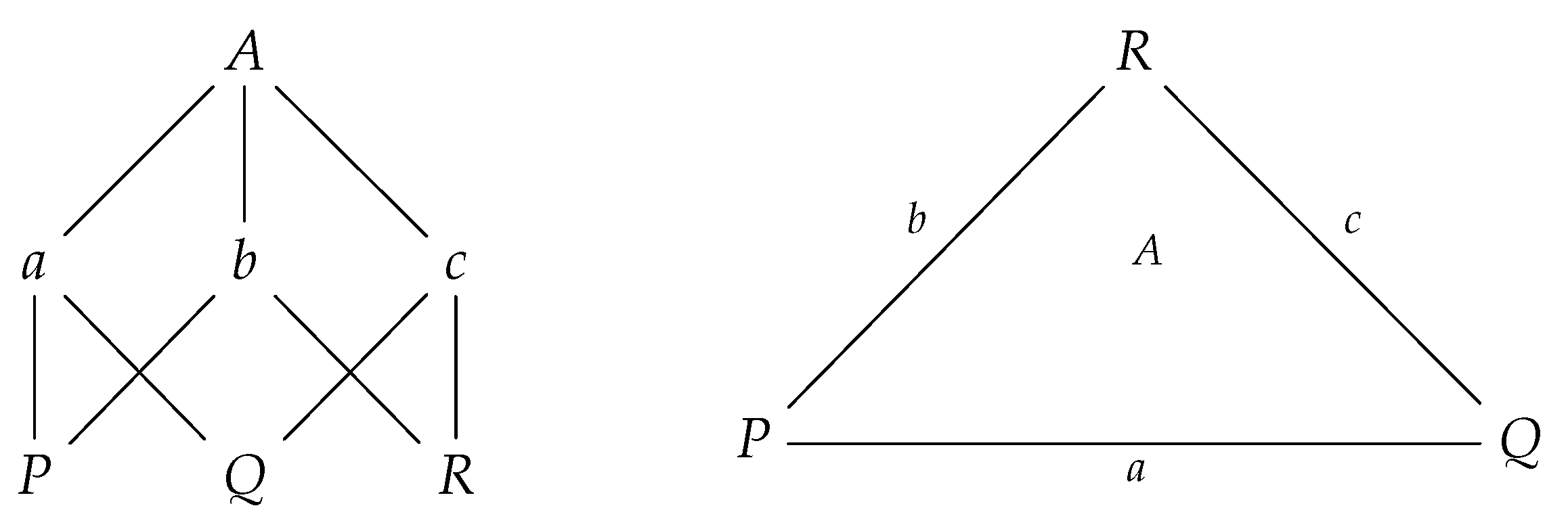
A minimal representation of the topology of a partially ordered set is given by the Hasse diagram, which depicts all direct relationships between elements in the partial ordering. The Hasse diagram is a minimal binary relation such that the reflexive and transitive closure of this binary relation gives back the partial ordering. An example Hasse diagram is given in Figure 1, which depicts the Hasse diagram of the face poset of a triangle.

This idea led to the notion of topological database, which encodes topological data into a relational database where the reflexive and transitive closure operation becomes a fundamental operator in relational algebra. More details can be found in [5].

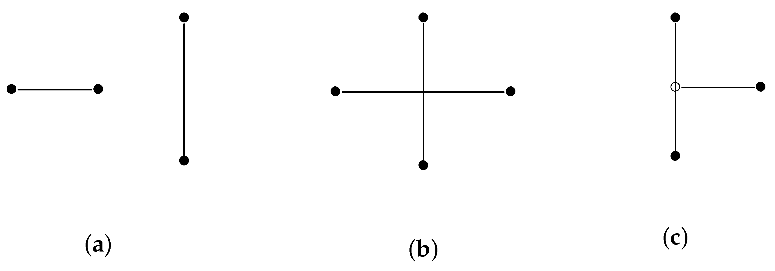
By assigning coordinates to the 0-dimensional simplices of a simplicial complex, it becomes a geometric model in Euclidean space. Special care must be taken if the model is to be topologically consistent (in the sense above), even if all points are given distinct coordinate tuples. For example, if a 1-dimensional simplicial complex (i.e., a simple graph) is given a geometry in this way, it can happen that, e.g., edges overlap. A complete list of the possible configurations of two line segments without common points is given in Figure 2. Notice that the solid points • in Figure 2 indicate that the point is explicitly modelled in the topology, whereas the hollow point ∘ indicates that it is modelled as a part of the horizontal line segment, but its intersection with the vertical line segment is not explicitly modelled in the topology. In the model topology, the two line segments are disjoint in all three cases.

If we assume that all simplicial complexes are of dimension two and that every point and edge is contained in the boundary of a triangle, then there are more possible topologically inconsistent configurations. For two triangles without common vertices or edges, there could possibly occur any one of the following intersections:

point–line; point–face; line–line; line–face; face–face.

The latter implies further topologically inconsistent intersections, such as line–line or point–line. Real-world examples where these occur are given and illustrated in [2].

A B-Rep is a common approach to explicitly store the topology of a model via the boundary relationships. However, it is prone to topological inconsistency, as has been demonstrated in [2]. Hence, if not carefully applied, the B-Rep representation can induce a loss of topological information. 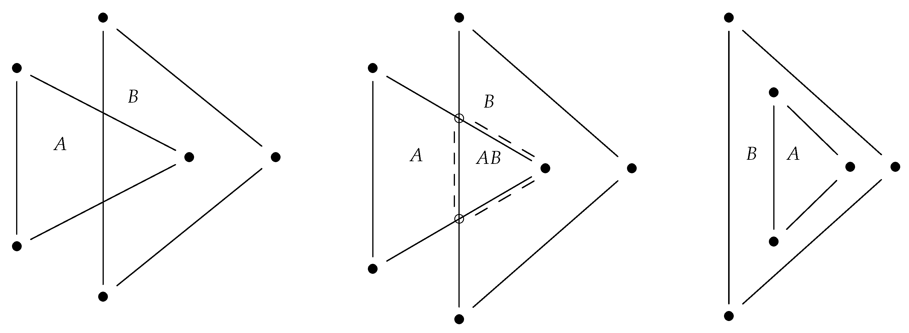Because of the spread of this carelessness, some data types, such as CityGML, approach this issue by using labels expressing a part-of relationship or a similar kind of semantics. Another issue is that a B-Rep does not model the interior of the object it represents—only its boundary. However, the interior cannot always be clearly inferred from the boundary, cf. Figure 3, left and right configuration. So, here, we may and will presume that a B-Rep does not always properly recover the topology.

In order to remedy this problem and to obtain topological consistency, we define the overlay of two topological objects X and Y. It is given by defining a topology on the set of intersections of the interiors and boundary objects of X and those of Y. Namely, for two such objects $x,y$, we define:

$$x⪯y$$

if either already x is in the boundary of y in X or Y (either old boundary or in the Euclidean topology) or if x is a subset of y geometrically. The latter case does not occur in the old topologies of X and Y, respectively, but in the new overlay topology. This new situation is for us a part-of relationship which extends the topology of the union $X\cup Y$. In the implementation, we distinguish between the old boundary relationships and the new Euclidean boundary and new part-of relationships in the overlay:

The intersection complex is then the structure of a cell complex on the geometric intersection given by the overlay complex.

Figure 3 illustrates the concept of overlay. On the left, there are two triangles consisting of points, lines and an interior A and B, respectively, and some objects of A have a non-empty intersection with objects of B. On the right, the overlay is given by the old objects plus six new objects: the two circle-points, the three broken lines and the interior area $AB$. The topology is given by the old boundary relationship in the union of the two triangles, plus the new Euclidean boundary and the new part-of relationships. The latter is given by: new circle-points are part of old lines, new broken lines are part of old broken lines and new area $AB$ is part of A and of B. The Euclidean topology shows us, e.g., that the circle-points, the broken lines and the bullet in the interior of B are all in the boundary of $AB$. The intersection complex in this example consists of the triangle $AB$ together with all its boundary elements. Observe that the overlay topology does not only consist of border-of relations but also contains part-of relations.

3.3. Euler Characteristic

Topological invariants play an important role in the characterization of topologies, in that if they are different, then the topological spaces are not homeomorphic, i.e., distinguishable from a topological point of view. An important set of topological invariants is given by the Betti numbers $b_i\left(X\right)$, which can briefly be explained as the numbers of independent holes of a given dimension i (the i-th Betti number), and was discussed in [9].

The Euler characteristic can be defined by the Betti numbers as follows:

Definition 1

(Euler characteristic topological). Let X be an n-dimensional cell complex built of only finitely many cells. Let $b_i\left(X\right)$ be the i-th Betti number of X with $i=0,\dots ,n$. The topological Euler characteristic can be defined as:

$${\chi }_{top}\left(X\right)=\sum _{i=0}^n{(-1)}^i{b}_i\left(X\right)$$

The Euler characteristic can also be defined by the number $c_m$ of m-dimensional cells of X with $m=0,\dots ,n$ as follows:

Definition 2

(Combinatorial Euler characteristic). Let X be an n-dimensional cell complex built of only finitely many cells. Let $c_m$ be the number of m-dimensional cells of X with $m=0,\dots ,n$. The combinatorial Euler characteristic can be defined as:

$${\chi }_{com}\left(X\right)=\sum _{m=0}^n{(-1)}^m{c}_m$$

Both definitions are equal if the cell complex X with only finitely many cells is topologically consistent (which is true by the definition of cell complex) and the cells of the cell complex X do not have holes. Practically, problems may occur due to computational geometry based on standard computational arithmetic (e.g., double precision) when calculating the geometrically induced topological overlay space $\overline{X}$. Some intersections may not be recognized, and others may not exist. Therefore, the results happen to be topologically inconsistent and the correctness of both Euler characteristics of those geometrically calculated unions are not always true. Furthermore, these two quantities may differ.

An n-dimensional sphere is the boundary of a $n+1$-dimensional ball. A cellulisation is a decomposition of a manifold to finitely many cells. A cellulisation of a ball can be deformed by flattening each cell to a polyhedron. Euler’s polyhedron formula states that any 3-dimensional polyhedron has Euler characteristic two. The generalized formula for n-dimensional spheres is given by the definition in [23] [Examples 0.2 and 0.3] via a representation of the sphere as a cell complex with precisely two cells:

Theorem 1

(General Euler’s polyhedron formula). Let X be a n-dimensional cell complex, which is a cellulisation of an n-dimensional sphere. Then, it holds true that:

$${\chi }_{com}\left(X\right)=1+{(-1)}^n$$

Therefore, a segment complex in the shape of the border of a polygon (1-dimensional sphere) has Euler characteristic zero. A triangle complex which is the triangulation of a polyhedron (2-dimensional sphere) has Euler characteristic two (original Euler’s polyhedron formula with $n=2$). A tetrahedron complex in the shape of a 3-dimensional sphere has Euler characteristic zero, etc.

In general, it is not a simple task to compute the Euler characteristic of a finite poset. The thesis [24] found a divide-and-conquer algorithm, but the time complexity of computing the Euler characteristic is still unknown, and possibly exponential in the number of points. For this reason, we approximate the topological Euler characteristic of the overlay space $\overline{X}$ with the combinatorial Euler characteristic:

$${\chi }_{top}\left(\overline{X}\right)\approx {\chi }_{com}\left(\overline{X}\right)$$

which can be expected to bring a great speed-up.

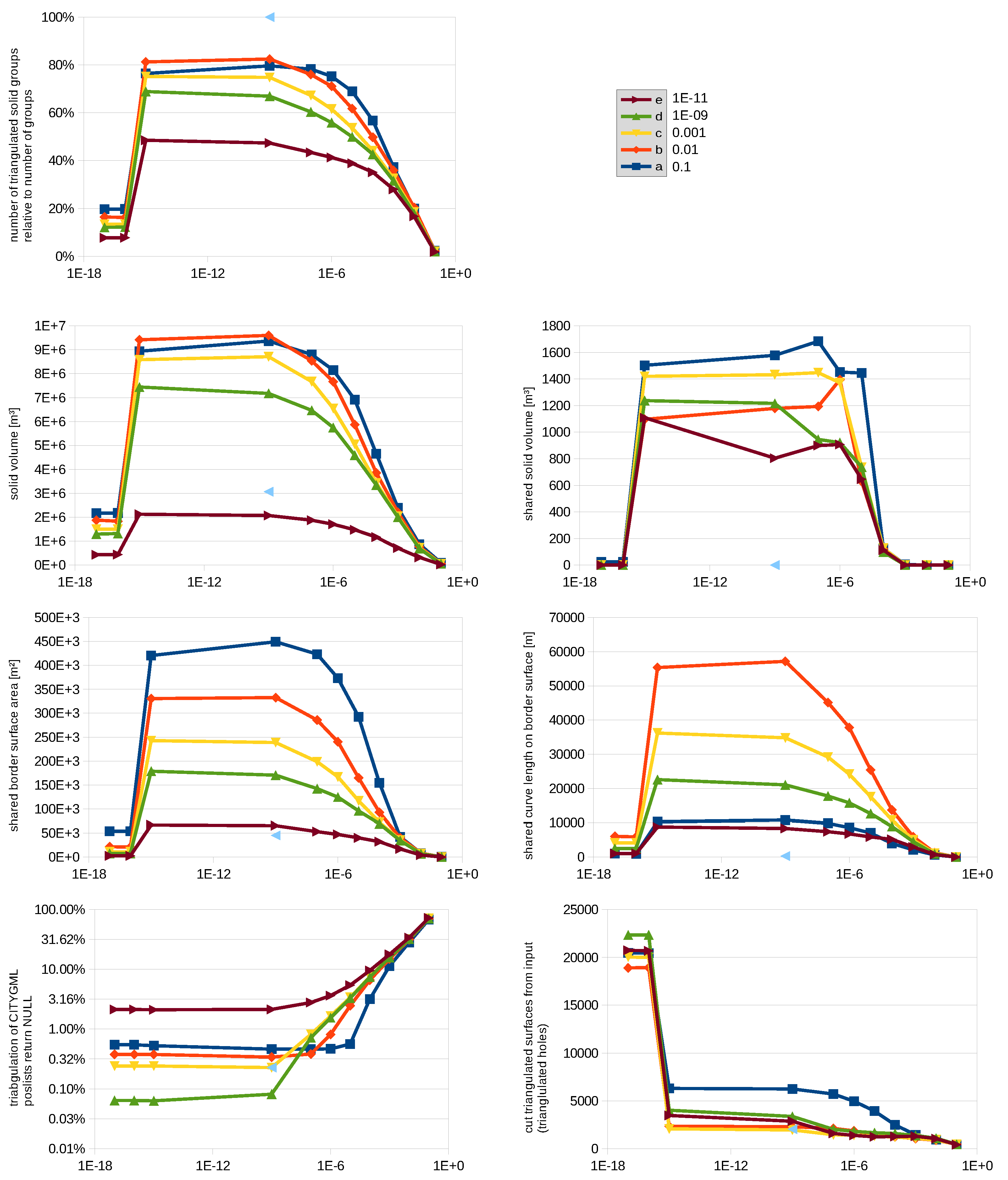
In our sensitivity and uncertainty study, we assume an uncertainty in the precision parameters, and this leads to a multitude of possible configurations which are either topologically consistent or not. In this way, one can determine the resulting topology or value of ${\chi }_{top}\left(\overline{X}\right)$ as a function of the precision parameters.

3.4. Algorithms

The used data model is described in [3,9,10], which also include a brief description of the used data model following the Property Graph Model, where special node properties have been added in order to support the Feature Model of the Open Geospatial Consortium (OGC). Algorithm 1 below, which calculates the disjoint inner of a set of intersecting d-dimensional simplicial complexes, has been introduced and visualized in [3]. Article [3] also includes some straight-forward algorithms to find the intersections or differences of simplicial complexes and provides certain triangulation algorithms of B-Reps based on double precision arithmetic with an epsilon heuristic inaccuracy model described in [20]. Article [3] did not include the description of the algorithms to find B-Reps from a set of d-dimensional simplicial complexes, which are thought to be topologically consistent, where the corresponding $T_0$-space is represented by a sub-set of the property graph, which is derived from the intersections of each d-dimensional simplicial complex with another. Those algorithms are discussed in the following.

Algorithm 1: Computing a set of $(d+1)$-dimensional simplicial complexes from a set of d-dimensional simplicial complexes—inner disjoint means that the interiors are disjoint.

input: set of d-dimensional simplicial complexes output: set of inner disjoint $(d+1)$-dimensional simplicial complexes 1 collect $(d-1)$-dimensional intersections; 2 create inner disjoint d-dimensional patch nodes; 3 create inner disjoint $(d-1)$-dimensional seam nodes; 4 stitch patch nodes which form manifolds and clean up; 5 stitch seam nodes which share the same patch nodes; 6 stitch patch nodes to form B-Reps and triangulate them to inner disjoint $(d+1)$-dimensional simplicial complexes; 7 create difference;

The complexity of finding all $(d-1)$-dimensional simplicial complex intersections in Step 1 depends on the used spatial access method for the n input d-dimensional simplicial complexes. There are m seams which are all $(d-1)$-dimensional intersections, the borders of each d-dimensional intersection and the borders of each d-dimensional simplicial complexes. Creating k inner disjoint d-dimensional patches for Step 2 depends on the dimension d. If $d=1$, it also depends on the spatial access method to retrieve the d-dimensional simplicial complexes, which need to be split by those m seams. In case of $d>1$, the complexity of Step 2 is equal to the complexity of Algorithm 1 with $d^{\prime }=d-1$ and m seams as input, since this algorithm creates the patches from the m seams recursively. The creation of the spatial access method for the patches needs to be considered within the calculation of complexity. The complexity of Step 3 depends on this spatial access method for k patches to find all l seams by intersecting each of the k patches with another. The creation of the spatial access method for the m seams needs to be considered, too. 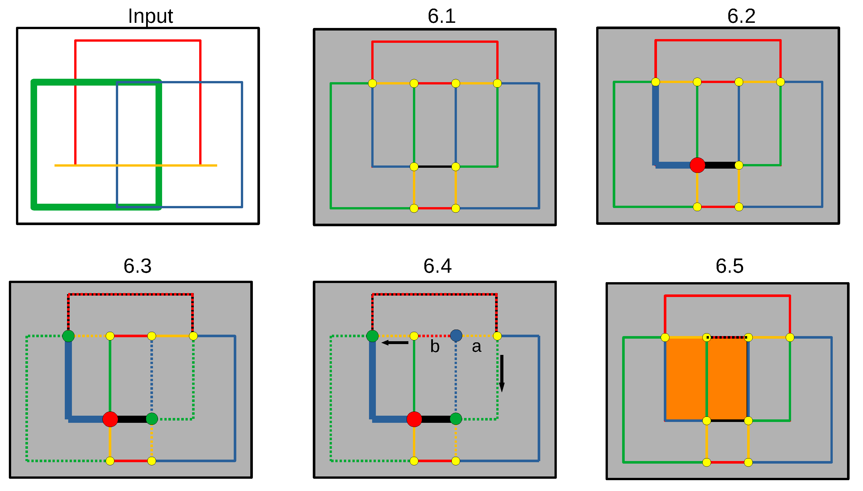Step 5 takes $\mathcal{O}\left(m\right)$ steps to glue patches to one manifold by iterating over the list of m seams. Step 6 to stitch patches to form valid B-Reps is parallelized for each seam through Algorithm 2. The complexity of Algorithm 2 will be discussed in the following paragraph. 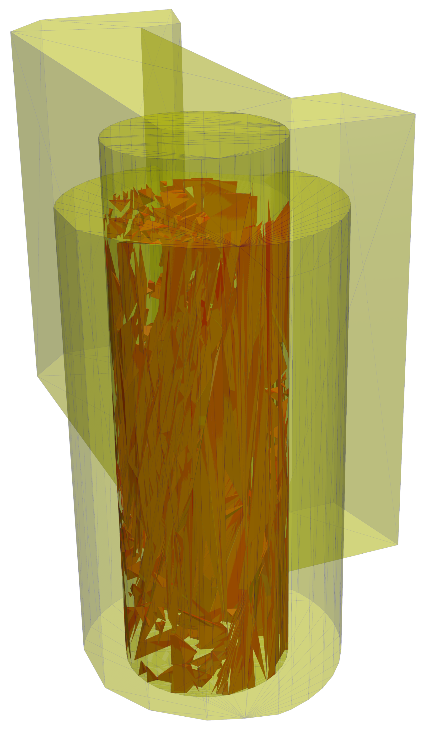Figure 4 illustrates Algorithm 2 of Step 6 of Algorithm 1. Step 7 of Algorithm 1 depends on the number of patches w that could not be connected to the $T_0$-space. The complexity to calculate the difference to the list of v inner disjoint $(d+1)$-dimensional simplicial complexes resulting from Step 6 of Algorithm 1 depends on the used spatial access method for v inner disjoint $(d+1)$-dimensional simplicial complexes queried by w patches. The creation of the spatial access method for v inner disjoint $(d+1)$-dimensional simplicial complexes also needs to be considered.

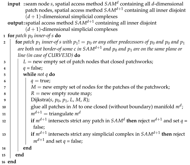
Algorithm 2: Run() operation of a thread for Step 6 of Algorithm 1—needs to run for every single seam node.

As mentioned before, Algorithm 2 describes how to find inner disjoint $(d+1)$-dimensional simplicial complexes for each pair of patches which are connected to one specific seam, which realizes Step 6 of Algorithm 1. In the 1-dimensional case, each patch is supposed to be a planar curve. Within the second FOR-loop (see Step 2 of Algorithm 2), patches $p_1$ will be rejected if it is not on the plane of $p_0$. If a plane cannot be defined by patch $p_0$ (patch lies on a straight line), a plane is defined by $p_0$ and $p_1$ for later checks within the Step 9. If a plane cannot be defined by patch $p_0$ and $p_1$, then every $p_{*}$ which will be determined within Step 9 may help to define a plane. If a plane was defined before, every $p_{*}$ will be ignored in Step 9 that does not lie on that plane. If not, and the union of all patches from Step 9 are not able to define a plane, then all patches are on a straight line, and a triangulation is not possible, since a straight line cannot be closed. However, the step to create a patchwork which can be triangulated to some $(d+1)$-dimensional simplicial complex is Step 9. This step will be discussed in Algorithm 3. After that step, the patchwork is glued to one closed (without boundary) d-dimensional simplicial complex and triangulated to a $(d+1)$-dimensional simplicial complex. If the patchwork could not be glued to one closed (without boundary) d-dimensional simplicial complex or the triangulation returned NULL, the algorithm does not try to find more closed (without boundary) d-dimensional simplicial complexes for the patches $p_0$ and $p_1$. If the triangulation was performed successfully, the resulting $(d+1)$-dimensional simplicial complex is tested as follows. If the resulting $(d+1)$-dimensional simplicial complex strictly contains any patch or strictly intersects any previously created $(d+1)$-dimensional simplicial complex (see Steps 12 and 13), the final patch that closed the corresponding d-dimensional simplicial complex within Step 9 is added to a set of patches for the patches that closed any of the previously generated patchworks. Those patches will be ignored for the next trials of Step 9.

Algorithm 3: Dijkstra(s, $p_0$, $p_1$, L, M, R) operation—Step 9 of Algorithm 2.

Step 9 of Algorithm 2 follows the idea of a Dijkstra algorithm with edge values of one as first straight forward implementation (see Algorithm 3) to find closed loops within the $T_0$-space. The set of loops represents balls containing the two patches $p_0$ and $p_1$ and the connecting border seam s. Any loop may fulfill the geometrical constraint (see Steps 12 and 13 of Algorithm 2). In fact, it is possible that the longest loop may fulfill the geometrical constraint only. Therefore, it is not the purpose to find the shortest loop here. It is a fact that most path-finding algorithm have a similar idea as Dijkstra’s, which is explained as follows. Let B be the set of borders from two patches $p_0$ and $p_1$ without the connecting border seam s. Algorithm 3 starts with this set of borders by the use of a Queue. This is a collection designed for holding elements prior to processing (with first in first out). The seam s functions as a barrier. Following the relations of the $T_0$-space, each border is connected to a set of patches. However, each border needs to be stitched to only two patches in order to fulfill the manifold constraint. The first patch is where the Dijkstra comes from, and the second patch is where the Dijkstra goes to. As mentioned before, in case the patches are planar curves, only patches are taken into account which lie on the previously defined plane. If a plane was not defined, each of the patches may help to define a plane. However, the patches themselves are bounded by some border seams also. Each patch will be added by Algorithm 4. If this algorithm returns “true” then the second patch closed the d-dimensional simplicial complex or a path back to some border(s) in B. Algorithm 4 returns “true” only if a non-self-intersecting loop was found. The patch is added to the set of patches M which represents the resulting patchwork. The complexity of Algorithm 4 depends on the number of interconnected borders and patches. The worst case would be that the non-self-intersecting loop with the most edges in the $T_0$-space forms the d-dimensional simplicial complex, which fulfils the constraints of Steps 12 and 13 of Algorithm 2.

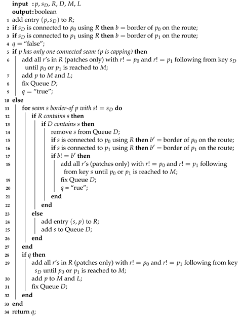
Algorithm 4: addPatch(p, $s_D$, R, D, M, L) operation—Step 12 of Algorithm 3.

Algorithm 4 checks if one of those new border seams was already visited and is connected to a different border seam within B. If so, a loop is found. It may happen that the second patch is bounded by only one border. This patch is like a capping and closes the border it is connected to the hole of the first patch. However, if a second patch like this or a loop was found, all the patches of this loop or the path back to the seam s are added to the result set M. If the second patch brings in some new borders, then they need to be closed in the same manner. Algorithm 4 filters the set of borders D which need to be visited in the next step of the Dijkstra if any second patch was found. All borders which contain any patches in M on their path back to the seam s are rejected. On the other hand, all new borders of the second patch need to be added to D if the second patch contains borders which need to be closed.

If a seam is connected to n patches, the complexity will be $\mathcal{O}\left(n^2\right)$ times the complexity within the two for loops (see Algorithm 2). If there are k closed (without boundary) d-dimensional simplicial complexes which can be triangulated to k$(d+1)$-dimensional simplicial complexes, then it takes $\mathcal{O}\left(k\right)$ steps to find the one which fulfills the two constraints (see Step 12 and 13) in the worst case. The worst case is that the d-dimensional simplicial complex consists of the maximal number of patches relative to the other d-dimensional simplicial complexes. This one would be found at last within the Step 9. The Dijkstra itself will take $\mathcal{O}\left(m\right)$ for m patches.

3.5. Decomposition Types

As described in [3,10] different ways of decomposing an XML based file (e.g., CityGML) exists by grouping geometries by an XML tag. Figure 5 shows examples. We choose the same decomposition types for this research as described in [3,10]. The first decomposition type tetrahedralises all buildings in one step. The second decomposition type tetrahedralises each building separately, and if the building is a collection of building parts, all the building parts will be tetrahedralised in one step. The third decomposition type tetrahedralises each building separately, and if the building is a collection of building parts, the building parts will also be tetrahedralised separately. Therefore, the first method leads to inner disjoint tetrahedron complexes which may share border objects. The second method leads to shared solid volumes between buildings, if the interiors of the tetrahedron complexes overlap. The third method also leads to shared solid volumes within buildings if the different tetrahedron complex interiors of the building parts overlap.

4. Experiments

4.1. The Influence of Double Precision Arithmetic

The focus of the sensitivity analysis lies on how many decompositions (buildings/building parts or buildings as a whole) are can be triangulated under a certain parameter setting. For geo-information purposes, shared solid volumes are calculated and the reciprocal speed up in percentage of a certain parallelization is also presented. The test parameters have been chosen from the inaccuracy model as follows. Only the factor ${\zeta }^{\prime }$ for cosine comparison and the base precision value $\alpha$ have been manipulated for the sensitivity analyses. The other factors have been set to the value of one. This implies that $ϵ=\epsilon =\sigma =\lambda$.

Figure 6 shows an overview of the data quality of some portions of the data released by the Thuringian state office for land management and geo-information (TLBG). The raw data are CityGML, which is a tree as a special case of a graph. Since the tree consists of 1,411,404 nodes with 109,224 distinct polygons (see second Figure 6 “LoD2-642-5648-2-TH”), we decided not to provide a figure in the form of a graph/tree. However, an example is given later on for explanation purposes in Figure 7 (left), which is part of "LoD2-642-5648-2-TH", and summarized in the first Figure 6, column “Krämer-Brücke”.

The sensitivity analysis has been calculated for the last quadrant of the second table in Figure 6, LoD2-642-5648-2-TH. The algorithmic pipeline is shown in Figure 8. An example is given in Figure 7 with $ϵ=\epsilon =\sigma =\lambda ={10}^{-1}$ and $\zeta ={10}^{-9}$. The set of segment complexes of a group is defined by the used decomposition type (left). Each segment complex is triangulated to a triangle complex (second from left). The next step is to start the parallel tetrahedralisation for each sub-node (see Figure 8 in red) by using a set of threads. The final set of inner disjoint tetrahedron complexes of each thread is created by calling the Algorithm 1 with the previously generated set of triangle complexes as the input set. The result can be seen in Figure 7 (second from right). The resulting set of inner disjoint tetrahedron complexes of each thread are added to one aggregation node. This node is the source node for the pipeline which creates the results for the sensitivity analysis.

The first step in the pipeline to create the results is to create each sub-node for each tetrahedron complex of the previously created aggregation node. All sub-nodes (see Figure 8 in yellow) are collected into one spatial access method (SAM) to support the next step. A thread pool calls the buildOverlay() operation on each sub-node to create the interior overlays in parallel. The buildOverlay(…) operation calculates all strict intersections (border intersections are ignored) with a set of given nodes. Each node-to-node intersection is linked to a new node, and the new node is related to its parents in an aggregation relation. The set of the resulting tetrahedral interior overlay nodes (see Figure 8 in green) are the shared solid volumes of the groups, since the Algorithm 1 for each group returned inner disjoint tetrahedralised tetrahedron complexes. The next step is to retrieve each border sub-node of each sub-node in order to calculate the border interior overlay of the set of border sub-nodes in parallel, just as the interior overlay calculation of the sub-nodes for the inner disjoint tetrahedron complexes previously. The set of the resulting border interior overlay sub-nodes (see Figure 8 in blue) are the shared border areas, curves and points of the border sub-nodes. The shared border areas, curves and points include the inner border areas, curves and points of all groups, since the tetrahedralisation of a group may result in the aggregation of several tetrahedron complexes (see previous paragraph). Figure 7 shows the intersection geometry (top right) and the whole resulting $T_0$-space (bottom right).

Figure 9 and Figure 10 show the results of the spatial analysis. Figure 11 and Figure 12 show the results of the processing times analysis.

The light blue triangle is a reference point from the first decomposition type when collecting all “planar” polygons (represented as B-Reps) of the input CityGML dataset into one aggregation, triangulating the set of segment complexes one after another, which creates a set of triangle complexes which in turn serves as the input for Algorithm 1. This first decomposition type (no decomposition) leads to inner disjoint tetrahedron complexes, as mentioned before over the whole CityGML dataset.

Figure 9 shows the results of the second decomposition type, which tetrahedralises each building separately. If the building consists of multiple parts, all “planar” polygons (represented as B-Reps) of the building are collected into one set of segment complexes. As mentioned before, this strategy may lead to shared solid volumes between buildings only, since the Algorithm 1 returns inner disjoint tetrahedron complexes for each group. Therefore, if the building consists of multiple parts, they will be integrated into the whole building solid, which consists of inner disjoint tetrahedron complexes.

Figure 10 shows the results for the third decomposition type, which separately tetrahedralizes each building or building part if the building consists of multiple parts. As mentioned before, this strategy may lead to shared solid volumes between buildings and/or building parts.

The top diagram of Figure 9 and Figure 10 show the relative number of solid groups to the number of groups. Both decomposition types show nearly the same percentage results. To understand the diagram, it is important to know that a group is counted as a tetrahedralised group if at least one valid tetrahedron was calculated by Algorithm 1. Precisions $ϵ=\epsilon =\sigma =\lambda >{10}^{-2}$ lead to more failures. The percentages rise with growing angular precision $\zeta$ and drop at ${10}^{-16}$. The maximum is at ${10}^{-9}$. The curves for each precision $ϵ=\epsilon =\sigma =\lambda$ value are relatively equal in shape but differ in their maximum. A value of $ϵ=\epsilon =\sigma =\lambda ={10}^{-2}$ and $\zeta ={10}^{-9}$ shows the highest maximum at nearly $90\%$ for the second decomposition type. As expected, this value is slightly higher than its counterpart in the third decomposition type. If one building part is not able to be tetrahedralised, it will not count within the third decomposition type, whereas a group of the second decomposition type, which contains all triangle complexes of the contained building parts, seems to have more chances to be tetrahedralised successfully. This contradicts the assumption that larger groups are more difficult to be tetrahedralised successfully. Having in mind that a group is tetrahedralised successfully if at least one valid tetrahedron could be found, the assumption becomes relativised.

The second diagram (left in second row) shows the overall volume of all tetrahedralised solids. The light blue reference (no decomposition) shows much less volume than its yellow counterpart at the same angular precision at both decomposition types. The shapes of the curves are relatively equal to the first diagram. Precisions $ϵ=\epsilon =\sigma =\lambda >{10}^{-2}$ lead to more failures. The second decomposition type shows generally smaller values than the third decomposition type. This may be caused by redundant volumes of overlaid building parts which are not part of the second decomposition type. It may also be caused by tetrahedralisations which have not been successfully calculated when using the second decomposition type and tetrahedralisations which have been successfully calculated when using the third decomposition type. The last two reasons are also the reasons why the shared solid volume shown in Figure 9 and Figure 10 (right in second row) does not explain the differences. The value of the light blue counterpart affirms the assumption that larger groups lead to more failures in the tetrahedralisation process, even if more groups are able to be tetrahedralised successfully.

The shared solid volume shown in Figure 9 (right in second row) of the second decomposition type is less than the shared solid volume of the third decomposition type shown in Figure 10 (right in second row). Where the second decomposition type shows up to 170 m³, the third decomposition type shows values up to 1700 m³. The third row illustrates the shared border areas and curves. Both are smaller in the second decomposition type, as well. These values are not comparable since it is unknown which solid volumes have been successfully tetrahedralised in both, either the one- or non-decomposition type.

The last row shows how many “planar” polygons (represented as B-Reps) of the input CityGML dataset were not triangulated through the pre-processing step before Algorithm 1 (left) and the number of rejected patches from the recursive call of Algorithm 1, which are not part of the input of Algorithm 1 (right). As expected, the pre-processing step fails more often on larger angular precision $\zeta$, since thinner triangles may be needed to triangulate a polygon which is represented as B-Rep, whereas the number of rejected patches grows on smaller values of the angular precision $\zeta$, since the difference between a patch and the input may not be “Null” due to a too-high precision (less collinear, less parallel, etc).

Figure 11 shows the processing times of the tetrahedralisation when using six threads to tetrahedralise the set of groups and three threads to build each decomposition type on an Intel® Core™ i7-7700K CPU @ 4.20 GHz × 8 for the second decomposition type. If the six threads are in the same part of the Algorithm 1 where they use three threads to solve that part (e.g., Step 6 of Algorithm 1), the total number of threads would exceed the maximal number of threads that are able to run in parallel on the test computer. Figure 12 shows the processing times for the third decomposition type. The light blue reference point of the first decomposition type (all in one) have been calculated with eight threads in Step 6 of Algorithm 1.

The reciprocal speed up itself has not been calculated. Only the processing times of each thread were summed up to estimate the sequential processing times. The sequential processing time may be faster since writing into the same spatial access method may cause delay times, which should not be considered when measuring the speed-up. However, this is only the case when each thread writes its results into the final spatial access method of tetrahedron complexes. Nevertheless, the overall processing times shown in the bottom left diagram show slightly higher times than $16.6\%$ which would be the best result when using six threads. The parallelization stays most of the time under $17\%$. The parallel processing times of Step 6 of Algorithm 1 with three threads were included in both overall processing time measurements.

The best reciprocal speed up of Step 6 of Algorithm 1 with three treads would be $33.3\%$. The third decomposition type is relatively close to the best value. The measured values are twice as high when using the second decomposition type. The light blue counterpart has nearly a perfect reciprocal speed-up with a value of $12.5\%$ with 8 threads. The values are not comparable since larger groups seem to cause more tetrahedralisation failures (see the solid volume diagram in combination with the shared solid volume diagram), which have a strong influence on the processing times since it is unknown which part of Algorithm 1 fails and breaks its processing.

4.2. The Influence of the Decomposition

The combinatorial Euler characteristics (see Definition 2 in Section 3.3) are calculated for the three different decomposition types of a city model and their calculable topological inconsistencies in order to analyse the topological differences of those three decomposition types.

We chose the values of $ϵ=\epsilon =\sigma =\lambda ={10}^{-2}$ and $\zeta ={10}^{-9}$, which produced the highest number of successful tetrahedralisations. The combinatorial Euler characteristics of each tetrahedralised tetrahedron complex, of each tetrahedron complex of their interior overlays and of each simplicial complex of their border interior overlays are calculated. The combinatorial Euler characteristics are also calculated for each set of simplicial complexes as the topological sum, which represent the whole tetrahedralised set of tetrahedron complexes or one intersection of only two tetrahedralised tetrahedron complexes or their border complexes. We will refer to those sets or topological sums in the following as *3DNet objects. The tetrahedralisation method was applied with the pre-processing step of splitting non-planar triangle complexes which were triangulated from the “planar” polygons (represented as B-Reps) of the input CityGML dataset. The input CityGML dataset is the same as in the last section.

The combinatorial Euler characteristics are calculated for each decomposition type presented as a distribution over the number of spatial objects which share the same combinatorial Euler characteristic. The first group of distributions are the distributions for the tetrahedralised tetrahedron complexes (see the last section, Figure 8 yellow box) of all three decomposition types. The second group of distributions shows the distributions of their topological sum, the Tetrahedron3DNet objects (see the last section Figure 8 second row middle box), which has only one member, trivially.

The spatial objects for the next two groups of distributions are created by the interior overlays of the tetrahedron complexes (see the last section, Figure 8 pipeline yellow to green box). Where the first group of those two groups of distributions consists of the distributions for the shared tetrahedron complexes and the second group consists of the distributions of the topological sums, the Tetrahedron3DNet objects, retrieved from the interior overlay of only two tetrahedron complexes. Each tetrahedron complex of each of Tetrahedron3DNet object counts also into the previously created general distributions of tetrahedron complexes. The spatial objects for the rest of the second group of distributions are created by the border interior overlays of each tetrahedron complex (see the last section Figure 8 pipeline yellow to blue box) grouped by their dimension. The groups of distributions for each dimension are also divided into two groups of distributions, one for the general d-dimensional simplicial complex distributions and one for the distributions of the topological sums, the *3DNet objects, retrieved from the border interior overlay of only two tetrahedron complexes. Each d-dimensional simplicial complex of each of *3DNet object also counts into the previously created general distributions of d-dimensional simplicial complexes.

As described in Section 3.3, the combinatorial Euler characteristic depends on the computational precision and may be wrong for the spatial objects. The following presentation of the results is a matter of inaccuracy.

Table 1, Table 2, Table 3, Table 4 and Table 5 show the distributions. Table 1 shows the distributions of the tetrahedron complexes of each decomposition type. Each tetrahedron complex seems to not be the border of a 3-dimensional sphere since there seems to be no tetrahedron complexes with an Euler characteristic of zero (see Section 3.3 Euler’s polyhedron formula of Theorem 1). Table 2 shows the distributions for the Tetrahedron3DNet objects of all decomposition types. Because each tetrahedron complex seems to have a combinatorial Euler characteristic of one (see Table 1), the combinatorial Euler characteristic could represent the number of tetrahedron complexes within the Tetrahedron3DNet objects.

4.2.1. Resulting Tetrahedron Complexes of the Interior Overlay of Each Tetrahedron Complex

Table 3 shows the distributions of tetrahedron complexes created by the interior overlay of each tetrahedron complex. There seem to be no tetrahedron complexes found by the first decomposition type. The other decomposition types show that each tetrahedron complex, created by the interior overlay, seems to not be a border of a 3-dimensional sphere since there seems to be no tetrahedron complexes with a combinatorial Euler characteristic of zero (see Section 3.3 Euler’s polyhedron formula of Theorem 1). Table 4 shows the distribution of Tetrahedron3DNet objects of the second decomposition type, and Table 5 shows the distribution of Tetrahedron3DNet objects of the third decomposition type. Because every tetrahedron complex seems to show a combinatorial Euler characteristic of one (see Table 3), the combinatorial Euler characteristic could represent the number of tetrahedron complexes within the Tetrahedron3DNet objects. There are Tetrahedron3DNet objects with many tetrahedron complexes. Figure 13 shows one of those Tetrahedron3DNet objects. Some tetrahedrons resulting from the interior overlay are not valid (e.g., too sharp or too small) and are cut out of the final result. The result should be a tetrahedron complex, but due to so many invalid tetrahedrons, the result is a Tetrahedron3DNet object with many tetrahedron complexes.

4.2.2. Resulting Triangle Complexes of the Border Interior Overlay of Each Tetrahedron Complex

Table 6 shows the first, second and third decomposition types with the distributions of triangle complexes. The first decomposition type shows that there should not be any hulls (2-dimensional sphere) since there seem to be no triangle complexes with a combinatorial Euler characteristic of two (see Section 3.3 Euler’s polyhedron formula of Theorem 1). The other two decomposition types show that most of the triangle complexes seem to have a combinatorial Euler characteristic of one. Some could shape hulls (2-dimensional sphere), which seem to show a combinatorial Euler characteristic of two (see Section 3.3 Euler’s polyhedron formula of Theorem 1). Table 7 shows the distribution of Triangle3DNet objects of the first decomposition type. Because it is known that the contained triangle complexes within each Triangle3DNet object seem to show a combinatorial Euler characteristic of one (see Table 6), the combinatorial Euler characteristics could represent the number of triangle complexes of the Triangle3DNet objects. Table 8 shows the distribution of Triangle3DNet objects of the second decomposition type, and Table 9 shows the distribution of Triangle3DNet objects of the third decomposition type. Because each of the contained triangle complexes within each Triangle3DNet object may not have a value of one (see Table 6), the combinatorial Euler characteristics should not represent the number of triangle complexes contained by each Triangle3DNet object. However, a Triangle3DNet object with higher Euler characteristics may indicate numerical errors due to the double precision arithmetic.

4.2.3. Resulting Segment Complexes of the Border Interior Overlay of Each Tetrahedron Complex

Table 10 shows the distributions of segment complexes created by the border interior overlay of each tetrahedron complex of the first, second and third decomposition type. The first decomposition type shows that there should not be any polygon boundaries (1-dimensional sphere), since there seems to be no segment complexes with a combinatorial Euler characteristic of zero (see Section 3.3 Euler’s polyhedron formula of Theorem 1). The other two decomposition types show that nearly one quarter of segment complexes seem to have a combinatorial Euler characteristic of zero, and the other two quarters seem to have a combinatorial Euler characteristic of one. The first decomposition type consists of only one Segment3DNet object. Because it is known that the contained segment complexes within the Segment3DNet object seem to show a combinatorial Euler characteristic of one (see Table 10), the combinatorial Euler characteristics should represent the number of segment complexes contained by this Segment3DNet object. Table 11 shows the distribution of Segment3DNet objects of the second decomposition type, and Table 12 shows the distribution of Segment3DNet objects of the third decomposition type. Because there seems to be one quarter with a combinatorial Euler characteristic of zero and three quarters with a combinatorial Euler characteristic of one (see Table 10), the combinatorial Euler characteristics most likely underestimates the number of segment complexes within the Segment3DNet objects.

4.2.4. Resulting Point Complexes of the Border Interior Overlay of Each Tetrahedron Complex

Table 13 shows the distribution of point complexes created by the border interior overlay of each tetrahedron complex of the first decomposition type. Only one point intersection exists within the first decomposition type. Table 14 shows the distribution of point complexes of the second decomposition type, and Table 15 shows the distribution of point complexes of the third decomposition type. The border of the tetrahedron complexes touch each other with a peak of 24, respectively 90, times. This may result from the failures in creating the overlay, as seen in Figure 13.

Table 1. First, second and third decomposition types (from left to right)—distributions of combinatorial Euler characteristics of tetrahedron complexes.

Euler	1	1	1
Count	3212	6703	7660

Table 1. First, second and third decomposition types (from left to right)—distributions of combinatorial Euler characteristics of tetrahedron complexes.

Euler	1	1	1
Count	3212	6703	7660

Table 2. First, second and third decomposition types (from left to right)—distributions of combinatorial Euler characteristics of Tetrahedron3DNet objects.

Euler	3212	6703	7660
Count	1	1	1

Table 2. First, second and third decomposition types (from left to right)—distributions of combinatorial Euler characteristics of Tetrahedron3DNet objects.

Euler	3212	6703	7660
Count	1	1	1

Table 3. First, second and third decomposition types (from left to right)—distributions of combinatorial Euler characteristics of tetrahedron complexes from interior overlay.

Euler	-	1	1
Count	-	518	2476

Table 3. First, second and third decomposition types (from left to right)—distributions of combinatorial Euler characteristics of tetrahedron complexes from interior overlay.

Euler	-	1	1
Count	-	518	2476

Table 4. Second decomposition type—distribution of combinatorial Euler characteristics of Tetrahedron3DNet objects from interior overlay.

Euler	2	3	4	5	7	8	9	10	14	16	17	18	23
Count	55	9	2	1	1	1	1	1	1	1	1	1	1

Table 4. Second decomposition type—distribution of combinatorial Euler characteristics of Tetrahedron3DNet objects from interior overlay.

Euler	2	3	4	5	7	8	9	10	14	16	17	18	23
Count	55	9	2	1	1	1	1	1	1	1	1	1	1

Table 5. Third decomposition type—distribution of combinatorial Euler characteristics of Tetrahedron3DNet objects from interior overlay.

Euler	2	3	4	5	6	7	8	9	10	11
Count	69	17	3	7	2	6	4	2	3	2
Euler	12	14	15	16	17	18	20	23	24	27
Count	1	3	2	1	2	1	3	1	1	1
Euler	28	30	36	37	40	41	42	45	105	1088
Count	1	1	1	1	1	1	1	1	1	1

Table 5. Third decomposition type—distribution of combinatorial Euler characteristics of Tetrahedron3DNet objects from interior overlay.

Euler	2	3	4	5	6	7	8	9	10	11
Count	69	17	3	7	2	6	4	2	3	2
Euler	12	14	15	16	17	18	20	23	24	27
Count	1	3	2	1	2	1	3	1	1	1
Euler	28	30	36	37	40	41	42	45	105	1088
Count	1	1	1	1	1	1	1	1	1	1

Table 6. First, second and third decomposition types (from left to right)—distributions of combinatorial Euler characteristics of triangle complexes from border interior overlay.

Euler	1	0	1	2	−1	0	1	2
Count	843	8	6040	6	1	10	7418	4

Table 6. First, second and third decomposition types (from left to right)—distributions of combinatorial Euler characteristics of triangle complexes from border interior overlay.

Euler	1	0	1	2	−1	0	1	2
Count	843	8	6040	6	1	10	7418	4

Table 7. First decomposition type—distribution of combinatorial Euler characteristics of Triangle3DNet objects from border interior overlay.

Euler	1	2
Count	2	1

Table 7. First decomposition type—distribution of combinatorial Euler characteristics of Triangle3DNet objects from border interior overlay.

Euler	1	2
Count	2	1

Table 8. Second decomposition type—distribution of combinatorial Euler characteristics of Triangle3DNet objects from border interior overlay.

Euler	2	3	4	5	6	7	10
Count	498	96	20	13	1	1	1

Table 8. Second decomposition type—distribution of combinatorial Euler characteristics of Triangle3DNet objects from border interior overlay.

Euler	2	3	4	5	6	7	10
Count	498	96	20	13	1	1	1

Table 9. Third decomposition type—distribution of combinatorial Euler characteristics of Triangle3DNet objects from border interior overlay.

Euler	2	3	4	5	6	7	9	11	13	16
Count	608	126	25	13	3	1	1	1	1	1

Table 9. Third decomposition type—distribution of combinatorial Euler characteristics of Triangle3DNet objects from border interior overlay.

Euler	2	3	4	5	6	7	9	11	13	16
Count	608	126	25	13	3	1	1	1	1	1

Table 10. First, second and third decomposition type (from left to right)—distributions of combinatorial Euler characteristics of segment complexes from border interior overlay.

Euler	1	0	1	0	1
Count	49	687	1841	842	2384

Table 10. First, second and third decomposition type (from left to right)—distributions of combinatorial Euler characteristics of segment complexes from border interior overlay.

Euler	1	0	1	0	1
Count	49	687	1841	842	2384

Table 11. Second decomposition type—distribution of combinatorial Euler characteristics of Segment3DNet objects from border interior overlay.

Euler	1	2	3	4	5
Count	30	265	47	4	2

Table 11. Second decomposition type—distribution of combinatorial Euler characteristics of Segment3DNet objects from border interior overlay.

Euler	1	2	3	4	5
Count	30	265	47	4	2

Table 12. Third decomposition type—distribution of combinatorial Euler characteristics of Segment3DNet objects from border interior overlay.

Euler	0	1	2	3	4	5	6	7
Count	1	39	348	60	12	2	2	1

Table 12. Third decomposition type—distribution of combinatorial Euler characteristics of Segment3DNet objects from border interior overlay.

Euler	0	1	2	3	4	5	6	7
Count	1	39	348	60	12	2	2	1

Table 13. First decomposition type—distribution of combinatorial Euler characteristics of point complexes from border interior overlay.

Euler	1
Count	1

Table 13. First decomposition type—distribution of combinatorial Euler characteristics of point complexes from border interior overlay.

Euler	1
Count	1

Table 14. Second decomposition type—distribution of combinatorial Euler characteristics of point complexes from border interior overlay.

Euler	1	2	3	4	5	6	7	8	9	10	11
Count	57	42	51	18	11	9	10	7	6	1	1
Euler	12	13	14	15	16	17	18	20	21	22	24
Count	6	1	1	2	2	3	3	1	1	1	3

Table 14. Second decomposition type—distribution of combinatorial Euler characteristics of point complexes from border interior overlay.

Euler	1	2	3	4	5	6	7	8	9	10	11
Count	57	42	51	18	11	9	10	7	6	1	1
Euler	12	13	14	15	16	17	18	20	21	22	24
Count	6	1	1	2	2	3	3	1	1	1	3

Table 15. Third decomposition type—distribution of combinatorial Euler characteristics of point complexes from border interior overlay.

Euler	1	2	3	4	5	6	7	8	9	10	11	12	13	14
Count	85	80	74	38	22	22	16	20	12	25	5	13	5	5
Euler	15	16	17	18	19	20	21	22	23	24	25	26	33	34	90
Count	3	7	4	13	2	1	1	1	1	1	1	1	1	1	2

Table 15. Third decomposition type—distribution of combinatorial Euler characteristics of point complexes from border interior overlay.

Euler	1	2	3	4	5	6	7	8	9	10	11	12	13	14
Count	85	80	74	38	22	22	16	20	12	25	5	13	5	5
Euler	15	16	17	18	19	20	21	22	23	24	25	26	33	34	90
Count	3	7	4	13	2	1	1	1	1	1	1	1	1	1	2

5. Discussion

The classical definitions on topological consistency found in the literature deal with the correct modelling of objects. What these definitions usually lack is the correct modelling of the incidence relationships. This is addressed in the ISO 191907 standard, which is equivalent to the definition used in this present work. Taking this into account allows one (in theory) to produce geometric and topological volume models with our methods that are suitable for simulation purposes. The remaining practical issues are the numerical problems when dealing with computational geometry. There exist several approaches to address those numerical problems by introducing different arithmetics or exact computational geometry [21]. However, topological invariants, such as the Euler characteristic, allow one to identify regions in the model which are problematic. However, due to the topological inconsistency, the easily computed combinatorial Euler characteristic using the object counts differs in general from the topological one using Betti numbers. So, the former is also an approximation of the topological Euler characteristic, as it is very likely to be inefficient to calculate Betti numbers of finite $T_0$-spaces.

The experiments show that there exists a good robustness range for topological and geometrical parameters with respect to angular precision, which seems to be the most important numerical sensitivity parameter. Simulations on CityGML models will still not be able to capture flows on the whole model, but only after the successfully rendering of large parts of the model. If we assume that the found solids are correct, then for good choices of the sensitivity parameters, more than 80% of the buildings or building parts can be used to create a topologically consistent solid model. The combinatorial Euler distribution helps to identify unusual geometrical and topological settings that need to be explored manually.

Concerning the topology of the volumetric models, the findings about the Euler characteristics indicate that there is a dependence of the resulting topology on the selected decomposition type. Trivially, the fact that Algorithm 1 returns inner disjoint solids always leads to a different global topology when used for different decomposition types. This is due to different intersection qualities of the decompositions and the computational geometry problems of intersection calculations within Algorithm 1 when applied to different sets of input data.

Concerning processing time, probably at the moment, the results point in the direction that a large-scale rendering can be performed in acceptable time only if the complicated parts of the model are left out. Large-scale rendering should in the future be able to produce data which are useful for simulation studies. This is potentially good news, as city models can then be used not only for visualization purposes but also for calculating various future scenarios under different environmental settings at different spatial scales. Future research should investigate the differences in the resulting topology depending on the uncertainty parameters, and more optimal parallelization methods for the rendering process in order to have a better handling of the more complex parts of a city model.

References

1. Gröger, G.; Plümer, L. CityGML—Interoperable semantic 3D city models. ISPRS J. Photogramm. Remote Sens. 2012, 71, 12–33. [Google Scholar] [CrossRef]
2. Giovanella, A.; Bradley, P.; Wursthorn, S. Evaluation of Topological Consistency in CityGML. ISPRS Int. J. Geo-Inf. 2019, 8, 278. [Google Scholar] [CrossRef] [Green Version]
3. Jahn, M.; Bradley, P. Computing Watertight Volumetric Models from Boundary Representations to Ensure Consistent Topological Operations. ISPRS Ann. Photogramm. Remote Sens. Spat. Inf. Sci. 2021, 8, 21–28. [Google Scholar] [CrossRef]
4. Breunig, M. On the Way to Component-Based 3D/4D Geoinformation Systems; Lecture Notes in Earth Sciences; Springer: Berlin/Heidelberg, Germany, 2001. [Google Scholar]
5. Bradley, P.; Paul, N. Using the relational model to capture topological information of spaces. Comput. J. 2010, 53, 69–89. [Google Scholar] [CrossRef]
6. Alexandrov, P. Diskrete Räume. Mat. Sb. 1937, 2, 501–518. [Google Scholar]
7. Breunig, M.; Kuper, P.; Butwilowski, E.; Thomsen, A.; Jahn, M.; Dittrich, A.; Al-Doori, M.; Golovko, D.; Menninghaus, M. The Story of DB4GeO—A Service-Based Geo-Database Architecture to Support Multi-Dimensional Data Analysis and Visualization. ISPRS J. Photogramm. Remote Sens. 2016, 117, 187–205. [Google Scholar] [CrossRef]
8. Breunig, M.; Bradley, P.; Jahn, M.; Kuper, P.; Mazroob, N.; Rösch, N.; Al-Doori, M.; Stefanakis, E.; Jadidi, M. Geospatial Data Management Research: Progress and Future Directions. ISPRS Int. J. Geo-Inf. 2020, 9, 95. [Google Scholar] [CrossRef] [Green Version]
9. Jahn, M.; Bradley, P.; Al Doori, M.; Breunig, M. Topologically consistent models for efficient big geo-spatio-temporal data distribution. ISPRS Ann. Photogramm. Remote Sens. Spat. Inf. Sci. 2017, 4, 65–72. [Google Scholar] [CrossRef] [Green Version]
10. Jahn, M. Distributed & Parallel Data Management to Support Geo-Scientific Simulation Implementations. Ph.D. Thesis, Karlsruhe Institute of Technology, Karlsruhe, Germany, 2021. [Google Scholar]
11. Giovanella, A. Automatische Redundanzfreie Generierung von Topologie aus Multidimensionalen Geographischen Datenbeständen. Ph.D. Thesis, Karlsruhe Institute of Technology, Karlsruhe, Germany, 2021. [Google Scholar]
12. Joksić, D.; Bajat, B. Elements of spatial data quality as information technology support for sustainable development planning. Spatium 2004, 11, 77–83. [Google Scholar] [CrossRef]
13. Li, S. On topological consistency and realization. Constraints 2006, 11, 3151. [Google Scholar] [CrossRef]
14. Kang, H.; Li, K. Assessing topological consistency for collapse operation in generalization of spatial databases. In Perspectives in Conceptual Modeling; Akoka, J., Ed.; Lecture Notes in Computer Science; Springer: Berlin/Heidelberg, Germany, 2005; Volume 3770. [Google Scholar]
15. Biljecki, F.; Ledoux, H.; Du, X.; Stoter, J.; Soon, K.; Khoo, V. The most common geometric and semantic errors in CityGML datasets. ISPRS Ann. Photogramm. Remote Sens. Spat. Inf. Sci. 2016, 4, 13–22. [Google Scholar] [CrossRef] [Green Version]
16. Zhao, J.; Stoter, J.; Ledoux, H. A framework for the automatic geometric repair of CityGML models. In Cartography from Pole to Pole; Buchroithner, M., Prechtel, N., Burghardt, D., Eds.; Lecture Notes in Geoinformation and Cartography; Springer: Berlin/Heidelberg, Germany, 2014. [Google Scholar]
17. Sindram, M.; Machl, T.; Steuer, H.; Pültz, M.; Kolbe, T. Voluminator 2.0—Speeding up the approximation of the volume of defective 3D building models. ISPRS Ann. Photogramm. Remote Sens. Spat. Inf. Sci. 2016, 3, 29–36. [Google Scholar] [CrossRef] [Green Version]
18. Sekulić, M.; Marinković, M.; Ivković, I. Spatial Multi-Criteria Evaluation Method for Planning of Optimal Roads Alignments, with Emphasize on Robustness Analysis. Int. J. Traffic Transp. Eng. 2021, 11, 424–441. [Google Scholar]
19. Crosetto, M.; Tarantola, S. Uncertainty and sensitivity analysis: Tools for GIS-based model implementation. Int. J. Geogr. Inf. Sci. 2001, 15, 415–437. [Google Scholar] [CrossRef]
20. Schirra, S. Precision and robustness in geometric computations. In Algorithmic Foundations of Geographic Information Systems. CISM School 1996; van Kreveld, M., Nievergelt, J., Roos, T., Widmayer, P., Eds.; Lecture Notes in Computer Science; Springer: Berlin/Heidelberg, Germany, 1997; Volume 1340. [Google Scholar]
21. Vetter, J.; Huhnt, W. Accuracy Aspects when Transforming a Boundary Representation of Solids into a Tetrahedral Space Partition. In Proceedings of the EG-ICE, Hybrid, Berlin, Germany, 30 June–2 July 2021; Abualdenien, J., Borrmann, A., Ungureanu, L., Hartmann, T., Eds.; Universitätsverlag TU: Berlin, Germany, 2021; pp. 320–329. [Google Scholar]
22. Biljecki, F.; Ledoux, H.; Stoter, J. Error propagation in the computation of volumes in 3D city models with the Monte Carlo method. ISPRS Ann. Photogramm. Remote Sens. Spat. Inf. Sci. 2014, 2, 31–39. [Google Scholar] [CrossRef] [Green Version]
23. Hatcher, A. Algebraic Topology; Cambridge University Press: Cambridge, MA, USA, 2002. [Google Scholar]
24. Renders, J. Finite Topological Spaces in Algebraic Topology. Master’s Thesis, Ghent University, Belgium, Brussel, 2019. [Google Scholar]
Figure 1. (Left): The Hasse diagram of the face poset of the triangle on the (right).
Ijgi 11 00224 g001
Figure 2. Two line segments whose explicit topology does not allow common points: (a) topologically consistent; (b) topologically inconsistent line–line intersection; (c) topologically inconsistent point–line intersection. Case (b) is missing the intersection point. Both lines should explicitly reference the intersection point within their definition. Case (c) misses the intersection point explicitly referenced by the vertical line.
Ijgi 11 00224 g002
Figure 3. (Left and middle): the overlay of two triangles; (right): configuration of two triangles with same B-Rep as (left).
Ijgi 11 00224 g003
Figure 4. Illustration of Algorithm 2, Step 6 of Algorithm 1. The input of Algorithm 1 is shown in the top right (5 segment complexes). The result of Steps 1–5 of Algorithm 1 is shown in 6.1 (patches are coloured, seams are yellow dots). There is also one triangulated grey surface already found, bounded by the black segment complex that did not intersect any of the other coloured segment complexes. Two patches (thick blue and black line) are connected through one seam (red dot) in 6.2. The goal is to stitch a patchwork with those two patches that forms a valid B-Rep. The idea is to follow the connected patches (dotted lines) on the green seams (see 6.3). One patch is ignored (black red dotted line). It was rejected in a former iteration. All yellow seams have to be checked in 6.4. Starting with the blue seam, two options are available (patch a in orange and patch b in red). Taking patch a first leads to an invalid loop since it maps to the same green seam of the black starting patch where the blue seam is connected to. This loop is ignored. Taking patch b leads to a valid loop since it maps to the green seam of the blue starting patch where the blue seam is not mapped to. The orange square can be triangulated and checked against any one dimensional intersection, which would indicate that the found surface is not a distinct surface in 6.5. Patch b is added to the list of patches which closed some invalid loop to be ignored when restarting at Step 6.2.
Ijgi 11 00224 g004
Figure 5. CityGML examples for decomposing an XML based file. If a finer-grained decomposition type does not exist, the next less fine-grained decomposition is used (red arrow).
Ijgi 11 00224 g005
Figure 6. Data quality at ϵ = ε = σ = λ = 10 3 and ζ = 10 9 .
Ijgi 11 00224 g006
Figure 7. Geometries in first row from left to right: CityGML segment complexes colored by group, triangle complexes colored by group, resulting tetrahedron complexes from Algorithm 1 colored by ID, result of the inner overlay of each tetrahedron complex and their borders colored by aggregation level. Sequence of T 0 -space extensions in second row from left to right: CityGML (black) with the segment complexes (top green headed ring) and their grouping (bottom cyan headed ring), triangle complexes (outer bottom cyan headed ring), whole resulting T 0 -space after overlay.
Ijgi 11 00224 g007
Figure 8. Pipeline to build one run of the sensitivity analysis. The “*” within the green box and the black box indicates that the SAM may contain multiple aggregation levels (e.g., single simplex, simplex complexes or simplex nets as the topological sum of a set of simplex complexes). The first “*” within the blue box indicates that the SAM may contain multiple dimensions (e.g., samples, curves and surfaces). The second “*” indicates the aggregation level.
Ijgi 11 00224 g008
Figure 9. Results of city centre of Erfurt, second decomposition type. The dataset is decomposed into several groups, where each group consists of one building together with its parts. (x-axis: angular precision ζ , different colours for each precision ϵ = ε = σ = λ value).
Ijgi 11 00224 g009
Figure 10. Results of city centre of Erfurt, third decomposition type. The dataset is decomposed into several groups, where each group consists of one building or one building part if a building consists of several building parts. (x-axis: angular precision ζ , different colours for each precision ϵ = ε = σ = λ value).
Ijgi 11 00224 g010
Figure 11. Results with six threads for the set of groups and three threads for each group of the city centre of Erfurt, grouping each building with its parts into separate groups (x-axis: angular precision ζ , different colours for each precision ϵ = ε = σ = λ value).
Ijgi 11 00224 g011
Figure 12. Results with six threads for the set of groups and three threads for each group of the city centre of Erfurt for grouping each building or building parts into separate groups (x-axis: angular precision ζ , different colours for each precision ϵ = ε = σ = λ value).
Ijgi 11 00224 g012
Figure 13. Result of an interior overlay as a Tetrahedron3DNet object (red) of two building parts tetrahedralised to two tetrahedron complexes (yellow) in the shape of cylinders. This is an example of a Tetrahedron3DNet object with many tetrahedron complexes of Table 5.
Ijgi 11 00224 g013
Publisher’s Note: MDPI stays neutral with regard to jurisdictional claims in published maps and institutional affiliations.