Abstract
Soil erosion worldwide is an intense, poorly controlled process. In many respects, this is a consequence of the lack of up-to-date high-resolution erosion maps. All over the world, the problem of insufficient information is solved in different ways, mainly on a point-by-point basis, within local areas. Extrapolation of the results obtained locally to a more extensive territory produces inevitable uncertainties and errors. For the anthropogenic-developed part of Russia, this problem is especially urgent because the assessment of the intensity of erosion processes, even with the use of erosion models, does not reach the necessary scale due to the lack of all the required global large-scale remote sensing data and the complexity of considering regional features of erosion processes over such vast areas. This study aims to propose a new methodology for large-scale automated mapping of rill erosion networks based on Sentinel-2 data. A LinkNet deep neural network with a DenseNet encoder was used to solve the problem of automated rill erosion mapping. The recognition results for the study area of more than 345,000 sq. km were summarized to a grid of 3037 basins and analyzed to assess the relationship with the main natural-anthropogenic factors. Generalized additive models (GAM) were used to model the dependency of rill erosion density to explore complex relationships. A complex nonlinear relationship between erosion processes and topographic, meteorological, geomorphological, and anthropogenic factors was shown.
1. Introduction
Soil erosion became the main factor in degrading a fertile layer of agricultural lands. Intensive land use combined with natural factors creates conditions for increased development of soil erosion, including rills, erosion furrows, and ephemeral gullies. Often, these erosion forms turn into permanent gullies, completely removing the area from agricultural turnover. Therefore, it is not surprising that researchers worldwide pay special attention to the study of soil erosion and, in particular, rill erosion.
Both field and mathematical methods are the main methods for studying soil erosion. The field method is very accurate in estimating the volume of erosion changes on local areas, which somewhat complicates the spatial interpretation of the results at the region or landscape levels. Such methods include the classical methods of reference sites, landmarks, microprofiling, and measuring the length and width of washouts with a tape measure. Reference sites allow estimating the direct volume of soil washed away from the territory, providing an opportunity to artificially change the conditions of the “environment” [1]. Based on the data from such sites, the data for creating mathematical models of soil erosion assessment, which will be discussed below, were obtained. The method of landmarks and microprofiling makes it possible to accurately estimate the depth of washout in representative sites [2]. Studies using these techniques helped find a strong correlation between the width of washout and its depth, which, in turn, estimates the volumes of soil washed away from the territory [3,4]. At present, geodetic methods based on relief reconstruction using scanning data or photogrammetry, both ground and airborne, are being developed to assess erosion. The most accurate results can be achieved using ground-based laser scanning data using reference points [5]. Researchers from all over the world manage to record in this way, not only gully [6] or rill [7] soil erosion but also micro-rill and sheet soil erosion [8], the changes of which are within the first millimeters. Unfortunately, it is problematic to use such technologies for direct monitoring in areas larger than 1 hectare. This problem is attempted to be solved using airborne laser scanning; however, this technology has its limitations related to the positioning of the scanning equipment for the subsequent alignment of the repeated survey. This fact immediately precludes the use of airborne scanning to evaluate the dynamics of micro-rill and sheet erosion, but it does allow for more or less automated estimation of the total length and width of rill and gully erosion. Different approaches are used for this. For example, the most common one is based on the threshold value of the number of digital elevation model (DEM) cells, from which runoff into neighboring cells is possible. Depending on the resolution of the initial DEM obtained from scanning data, this approach allows recognizing rills depths from 5 cm. However, airborne laser scanning is not widely used due to the high cost of the scanning equipment. Nowadays, more affordable scanning sensors appeared installed on manned aircraft and unmanned aerial vehicles (UAV). Nevertheless, the applicability of such devices for solving the problem of soil erosion assessment has yet to be discovered—the analysis of the existing experience has demonstrated that the most significant relevance of such devices is in forestry [9]. Despite the current trend toward cheaper scanning systems, they are still not widely available to most researchers. Combining these factors has led to the most widespread use of photosensors as payloads for UAVs [10]. UAV photogrammetry makes it possible to achieve comparable point cloud densities with scanning systems’ competitive accuracy of the resulting models and allows one of the end products to be an ultra-high-resolution orthophotoplane. The use of UAVs makes it possible to provide geomorphological surveys with up-to-date information about the condition of the survey area cheaply, quickly, and accurately enough. Unfortunately, despite the overall high productivity, the use of UAVs does not allow for making a continuous survey of large regions [11,12]; however, it will enable verification model data.
Model data obtained from office studies make it possible to estimate the intensity of exogenous processes at both local and global levels. A whole range of mathematical models has been developed to assess soil and gully erosion, subdivided into empirically and physically based [13]. The most well-known and widely used soil erosion models are USLE [14], RUSLE [15], MUSLE [16], CREAMS [17], LISEM [18], and so on. WEPP [19], RillGrow [20], GUEST [21,22], and EUROSEM [23] models are used to estimate rill erosion. All these models have their advantages and disadvantages, and the latter does not allow using these models everywhere. The main limitations are related to the lack of publicly available large-scale remote sensing data [24], such as terrain models [25] and detailed comparable climate data [26,27], which does not allow the mathematical simulations needed to map streamflow paths. The lack of detailed remote sensing data also limits the possibility of applying object-oriented recognition of rill erosion [28] and stochastic modeling of erosion exposure [29,30].
The data obtained by erosion models in the form of erosion and accumulation balances often do not reflect the actual development of rill erosion processes. For example, in the catchments of the European part of Russia, it is not uncommon that the rate of accumulation in the bottoms of dry valleys tends to decrease [31,32,33], while the number, total length, and, accordingly, the density of rill network increases from year to year [34]. This is often due to the peculiarities of plowing with the creation of special sloughs that retain runoff from the fields, corrupting the results obtained by erosion models.
Considering the existing limitations, approaches based on manual extraction of washouts from remote sensing data, namely space images [35,36], are applied to solve the problem of rill erosion mapping. Remote sensing mapping of rill erosion was carried out using Landsat-5 (30 m) [37,38], QuickBird (0.6 m) and SPOT (5 m) satellite imagery [39], GeoEye-1 stereo pair [40], and UAV data [41]. Sentinel-2 (10 m) images were also used to create NDVI-images during the predictive model development [42], but the mapping has not been carried out directly based on them before. Such solutions allow for achieving the best accuracy but are labor consuming and low productive. To solve this problem, the development of approaches based on the automation of rills washout extraction is necessary, which is the goal of this work. The source data used as a cartographic basis sets a list of possible approaches that can be applied to solve the purpose. The simplest of them is object recognition based on a thresholding approach, where the threshold defines the boundary of the reflectivity of the spectral data characteristic of the study object. Such methods are suitable for identifying different land-use types [43,44]. However, the result will be unpredictable when recognizing rills using a similar approach on different types of soils. Machine learning methods can be used to consider the spatial variability of environmental factors, such as the highly proven Random Forest or Support Vector Machine method [45,46]. However, such approaches only give a probability of soil erosion in a particular pixel, while not distinguishing the erosions themselves into a “tree-like pattern” in the landscape. In addition, the methods are very sensitive to the amount of input data—the more information used for analysis, the more consistent the results will be. On small watersheds, such approaches can be successfully applied; for large areas, their applicability is questionable.
Recently, there has been a rapid increase in the number of works related to deep neural networks (DNNs) for the semantic segmentation of remote sensing data. This has been facilitated by the increased quality of remote sensing data, user-friendly deep-learning framework availability, and the increased computing power available to researchers. At present, DNNs enable successful automated interpretation of anthropogenic objects [47,48,49], shorelines [50,51], land use [52,53,54], vegetation cover dynamics [55,56], and exogenous processes [57,58]. In all cases, the authors note the higher recognition accuracy of the objects of interest than other methods and emphasize scaling the trained models. Deep neural networks have not been applied to the recognition and mapping of rill erosion. Nevertheless, the importance of the problem under study and the promising use of artificial intelligence for solving this problem determines the necessity of developing an appropriate methodology.
Given the intensification of rill erosion, the necessity of mapping it, and the limitations of field survey and modeling, this study aims to develop and apply a deep neural network-based methodology for automated rill erosion detection from remote sensing data.
2. Study Area
The study area is the Middle Volga region of Russia. The territory is located in the central part of the East European Plain [59]. The Middle Volga region’s agro-industrial complex (AIC) is of all-Russian importance. The region holds one of the top places in the country to produce grain, including the valuable grain crop—wheat. Agriculture is characterized by high efficiency due to very favorable natural conditions. At the same time, the agricultural sector of the territory has a substantial impact on natural-territorial complexes, primarily on the soil cover. Given the intensity of plowing, cattle grazing, and natural conditions conducive to the development of exogenous processes, this area is highly affected by soil erosion. This situation is not new; it is not accidental that the territory of the Middle Volga region is historically called an erosion belt. At the same time, anti-erosion measures in recent decades are of a point and haphazard nature, mainly due to the poor study of the rate and development direction of the process, primarily rill erosion.
The study area is 345,477 sq. km. The macroregion includes Mari El, Tatarstan, Chuvashia, Saratov, Samara, Ulyanovsk, and Penza regions. The Middle Volga region is located in the forest landscape zone in the north, the forest-steppe landscape zone in the center, and the steppe landscape zone in the south (Figure 1).
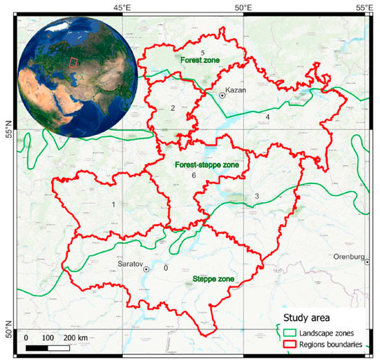
Figure 1.
The study area. The 0—Saratov region, 1—Penza region, 2—Republic of Chuvashia, 3—Samara region, 4—Republic of Tatarstan, 5—Republic of Mari El, and 6—Ulyanovsk region.
The relief of the Middle Volga region has a spotted asymmetry of slopes: the average height—146 m, maximum elevation—316.8 m, and minimum—13.2 m [60]. The region’s climate is moderately continental and continental in the south, varying wildly from region to region. Average annual precipitation ranges from 471 to 549 mm in the north to 264–424 mm in the south.
The steepness of the slopes of the territory, in general, is favorable for agriculture; a quarter of the region is steep to 1 degree, and a significant part of the territory is characterized by steepness in the range of 1–2.5 degrees, rising to 5 degrees in the area of Bugulminsko-Belebeyevskaya upland [60]. Erosion risks are not uniform and vary from region to region [61]. Soil-forming rocks are not homogeneous and are mainly clayey and heavy loam. There are sandy soils and medium-loam in the north of the Republic of Mari El region and light loam in the forest-steppe zone (Penza Oblast). Soils vary; chernozems of various subtypes predominate, mostly leached (Haplic Chernozems), as well as ordinary (Calcic Chernozems), typical (also Haplic Chernozems), and southern (Haplic Chernozems too)(steppe soils). The remaining types have a clearly expressed zonal pattern, where the gray forests (Haplic Greyzems) are typical for the forest territories and north of the forest-steppe zone [60].
3. Materials and Methods
The development and implementation of a methodology for automatic rill erosion recognition involve several interrelated points:
- Selection and preparation of remote sensing data from space;
- Preparation of training and test sets;
- Training the neural network and evaluating the quality of rill recognition;
- Implementation of the neural network for the entire study area and vectorization of recognition results;
- Calculation of rill erosion length as a measure of rill erosion density index in the basins;
- Analysis of the obtained results.
3.1. Remote Sensing Data
Data from the Sentinel-2 satellite constellation was used for recognition. Unlike other sources of multispectral remote sensing data, such as Landsat, MODIS, SPOT, RapidEye and so on, Sentinel-2 imagery provides the best resolution in the target bands (10 m) at no charge. The cloudless composite data of the Sentinel-2 mission for the spring period, April-June, were used as input data to develop the rill erosion recognition technique. Near-infrared images with baseline resolution (10 m) were used for recognition. The composite was created using the Google Earth Engine (GEE) [62], product “Sentinel-2 MSI: MultiSpectral Instrument, Level-2A” (COPERNICUS/S2_SR). GEE allows the processing of big remote sensing data and facilitates some routine operations. A total of 2988 scenes from both S2A and S2B satellites were used to create the composite. To create the composite, the 2018–2019 images were filtered by date, images were cleaned from clouds and shadows, median pixel brightness values were calculated, and imagery was clipped to the boundaries of the study area and reprojected into the WGS 84/Pseudo-Mercator (EPSG:3857) projection coordinate system. A cloud probability raster was used to clear the imagery from the clouds. The S2 cloud probability is created using the sentinel2-cloud-detector library (LightGBM [63]). All bands are upsampled using bilinear interpolation to 10 m resolution before the gradient boost base algorithm is applied. The resulting 0 to 1 floating point probability is scaled to 0–100 and stored as a UINT8. Areas missing any or all of the bands are masked out. Higher values are more likely to be clouds or highly reflective surfaces (e.g., roof tops or snow). A 15% probability of having clouds on the scene was used as the cloud threshold.
3.2. Preparation of the Training Dataset
In the resulting spring composite, an area with visually the densest rill network and the presence of major land-use classes of water, anthropogenic, forest, and agricultural features was selected and clipped. For this area of more than 2500 square kilometers, continuous manual rill erosion recognition was performed to create a set of reference data samples (Ground truth, GT) (Figure 2). Manual recognition was made by QGIS tools using Sentinel-2 data and ultra-high resolution (UHR) images (Bing, Google, and so on, available as a substrate at no charge). The main selection was made on the S2 images. In controversial cases, the UHR images were used. They were also used for the non-selection of permanent gullies. Due to the difficulty of classifying erosion forms on such a vast territory with different natural conditions, the differentiation of erosion forms was not carried out. Ephemeral gullies” and “rills” were defined as all erosion forms that can be interpreted on satellite images but do not belong to permanent gullies. Considering the resolution of the satellite image, rills are the most minor erosion form, which transforms into an ephemeral gully.
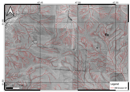
Figure 2.
Fragment of a rill erosion ground truth data (GT).
The resulting sample was rasterized and reduced to the resolution of the satellite image fragment, and then both images were cut into 256 × 256 pixels patches. In total, 10,933 satellite image-binary mask pairs have been obtained this way (Figure 3). The resulting rasters were further randomly transformed to augment the number of rasters by three times artificially. The resulting dataset was divided into training and test sets in the ratio of 1/5.
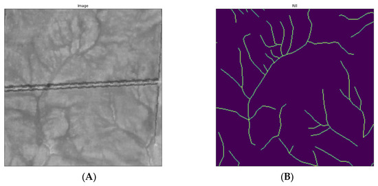
Figure 3.
Example of a satellite image patch (A) and a binary mask (B) of rill erosion.
3.3. Training a Deep Neural Network
A convolutional neural network is a class of artificial neural network that uses convolutional layers to filter inputs for useful information. The convolution operation involves combining input data (feature map) with a convolution kernel (filter) to form a transformed feature map. The filters in the convolutional layers (conv layers) are modified based on learned parameters to extract the most useful information for a specific task. Convolutional networks adjust automatically to find the best feature based on the task. Applications of convolutional neural networks include various image (image recognition, image classification, video labeling, text analysis) and speech (speech recognition, natural language processing, and text classification) processing systems, along with state-of-the-art AI systems, such as robots, virtual assistants, and self-driving cars.
LinkNet (Figure 4), a fully convolutional neural network for semantic image segmentation, was chosen as a neural network architecture [64]. In contrast to the well-known and well-proven U-NET architecture [57], which has been used for semantic segmentation of satellite images in geomorphological studies [65], LinkNet uses residual blocks instead of convolutional blocks in its encoder and decoder networks. The LinkNet deep neural network architecture efficiently exchanges the information received by the encoder with the decoder after each downsampling block. This turns out to be better than using pooling indices in the decoder, or just using fully convolutional networks in the decoder. This feature transfer technique not only gives good accuracy, but also allows a small number of parameters to be used in the decoder.
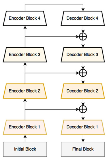
Figure 4.
DNN LinkNet architecture scheme [64].
The initial block contains a convolution layer with a kernel size of 7 × 7 and a stride of 2, then a max-pool layer with a window size of 2 × 2 and a stride of 2. Similarly, the last block performs a full convolution, taking feature maps from 64 to 32, then a 2D convolution. Finally, a full convolution is used as a classifier with a kernel size of 2 × 2. As practice has shown, this allows for better semantic aggregation, including dendro-like constructions (tree-like patterns on the landscape) and rill networks. By trial-and-error method, it became clear that the best results in decoding rills can be achieved using transfer learning, a deep neural network learning method that allows using the knowledge obtained about one deep learning problem and applying it to another, but with a similar problem. The encoders used for DenseNet image classification [66] were used in our case. In contrast to similar models, the features are not summed up but concatenated (channel-wise concatenation) into a single tensor before passing them to the next layer. The model learning and implementation algorithm was performed in the Python 3.7 programming environment using the Tensorflow library. The input of the neural network was a stack of image-mask pairs prepared in the previous step. EarlyStopping monitoring was used to prevent overtraining of the model, and the IOU Score metric, Jaccard’s coefficient, was used to check the model’s learning capability [67].
3.4. Statistical Analysis of the Obtained Results
Further research was conducted to analyze the influence of various natural–anthropogenic factors on the intensity of erosion processes in the study area. Classical correlation, regression analysis, and analysis of variance (AOV) (one-way [68] and multivariate [69]) were used to analyze the relationship between natural and anthropogenic factors on the density of the rill network. The AOV was performed using the Statsmodel package for Python 3. To analyze complex relationships, an analysis based on generalized additive models was used. The generalized additive model (GAM) is a generalized linear model in which a linear predictor depends linearly on unknown smooth functions of some predictor variables, and interest is focused on inference about these smooth functions. GAM uses spline functions, functions that can be combined to approximate arbitrary functions. GAM introduces penalties for the weights so that they remain close to zero, which effectively reduces the flexibility of the splines and reduces the possibility of overfitting. The smoothness parameter, which is normally used to control curve flexibility, is then adjusted using cross-validation. The natural–anthropogenic factors presented in Table 1 [60] were used for the analysis.

Table 1.
Natural–anthropogenic factors of rill erosion selected for analysis [60].
4. Results and Discussion
The trained RECNN (rill erosion convolutional neural network) was tested on an independent test dataset. The recognition accuracy was 0.62, F1-measure was 0.76, and loss-function was 0.27. Qualitatively analyzing the obtained evaluation results (Figure 5), we can note a relatively high level of recognition of the rill erosion network. It is crucial that not a single case of detection of gullies or ground roads, which are abundant in the study area, instead of rills, was recorded.
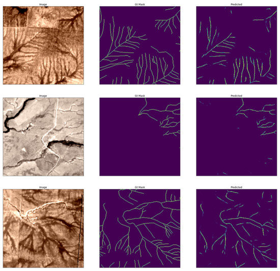
Figure 5.
An example of the results of applying RECNN to a test dataset.
The trained and tested model was decided to apply to the entire study area (Figure 6). For the obtained geometry, the length was calculated, which was aggregated to a grid of basins [60] (Figure 7). Analyzing the obtained maps, the presence of specific clusters becomes evident. The first cluster—the highest density of rill erosion—is located in the left-bank part of the Volga River in the Saratov region. The second cluster—the area of medium erosion—characterizes the right bank of the Volga in the Saratov region and Zakamye of the Republic of Tatarstan. The Republics of Mari El and Chuvashia territories are characterized mainly by low rill erosion, forming the third cluster.
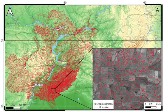
Figure 6.
Results of rill erosion recognition over the entire study area (A) and enlarged area with recognized streams in Sentinel 2 image (B).
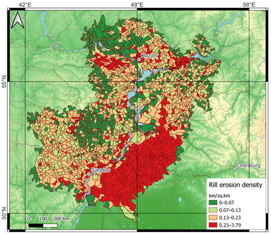
Figure 7.
Map of rill erosion density. Quartiles calculate intervals.
In total, information in the study area is aggregated on 3037 basins with an average area of 117.83 sq. km. The average density of rill erosion over the entire study area is 0.23 km/sq. km, and the maximum density is 3.79 km/sq. km. In general, the distribution of the total length of rill erosion in the study area is lognormal; that is, most of the measurements contain, in general, relatively small values of the total length (Figure 8).
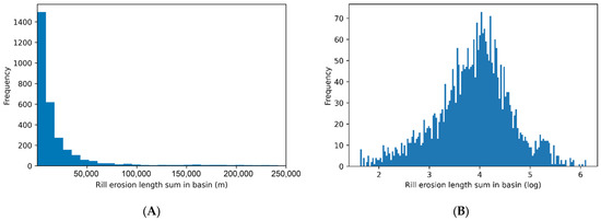
Figure 8.
Distribution of total rill erosion length (m) (A) and normalized distribution of total rill erosion length (B).
For most of the selected factors, no strong correlations were found with the total length of rill erosion. Only some factors revealed statistically significant (p < 0.001) weak relationships (r > |0.3|). For example, an inverse correlation describes the relationship between total rill erosion length and forest cover, hydrothermal coefficient, mean annual precipitation, mean May-August precipitation, and mean warm-season precipitation. The inverse relationship with forest cover is more than obvious and only states a well-known fact—the less forest cover of the territory, the greater the risk of soil and gully erosion. The inverse relationship with the other indicators is not so obvious. Selyaninov’s hydrothermal coefficient of wetness (GTK) is a characteristic of the level of moisture availability of the territory. It is widely used in agronomy for general climate assessment and allocation of zones with different levels of moisture availability to determine the usefulness of the cultivation of various crops. The factor is closely related to the amount of precipitation in the territory. The inverse relationship here is explained not so much by the very nature of the dependence “the more precipitation, the less erosion”, which cannot be, as by the influence of climatic conditions in general. This is partly confirmed by a direct relationship between the total length of the rill network and such factors, such as the sum of active temperatures and the average annual maximum temperature for the year. Apparently, with increasing temperature and climate change due to global warming, the character of precipitation changes—they may fall rarely, but with great intensity [70,71,72,73,74]. Unfortunately, it is impossible to check this hypothesis directly due to the lack of data on mean annual precipitation intensity changes. However, the same conclusions are drawn by other researchers who have worked in the study area [31,32,75,76]. Nevertheless, there is still no clear answer to this question.
Another question is how classical methods of relationship analysis can assess the effect of a single factor on the dependent variable. Linear dependencies are rare in nature, and polynomial dependencies of high degrees are even rarer. The analysis demonstrated poor applicability of classic correlation and regression analysis for revealing the relationships between natural–anthropogenic factors and the length of the erosion network. Some examples (Figure 9, Figure 10 and Figure 11) demonstrate that the dependencies are close to the logistic or exponential type but more complex. Therefore, it was decided to use generalized additive models (GAM) for dependence analysis [77]. These models allow estimating the dependencies in the form of spline functions, which allows one to make better approximations and comprehensively study the dependence of a factor on a variable [24,78].
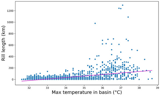
Figure 9.
Linear relation of the total length of rill erosion to maximum air temperatures.
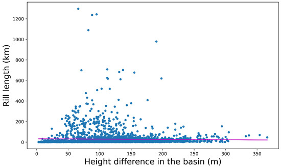
Figure 10.
Linear relation of the total length of rill erosion to the elevation variation in the basin.
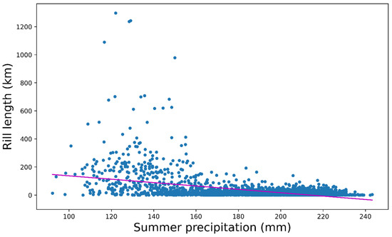
Figure 11.
Linear relation of the total length of rill erosion to mean annual precipitation from May to August.
Modeling of generalized relationships was performed in a package for building generalized additive models in the Python language [79]. During modeling, statistically significant (p < 0.001), stable, and strong relationships were found between the density of rill erosion and such natural factors as mean basin elevation (Figure 12A), mean basin slope (Figure 12B), basin elevation range (Figure 13A), basin forest cover (Figure 13B), average air temperature in January (Figure 14A), average annual long-term maximum temperature (Figure 14B), average warm-season precipitation (Figure 15A), average basin hydrothermal coefficient (Figure 15B), longitude (Figure 16A), and latitude (Figure 16B) of the basin centroid.
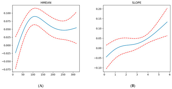
Figure 12.
Dependence of rill erosion density on topography factors—average height (m) (A) and average slope steepness (deg) (B) in the basin.
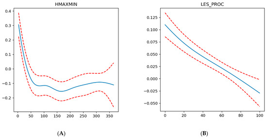
Figure 13.
Dependence of rill erosion density on elevation range (m) (A) and average forest cover (%) (B) in the basin.
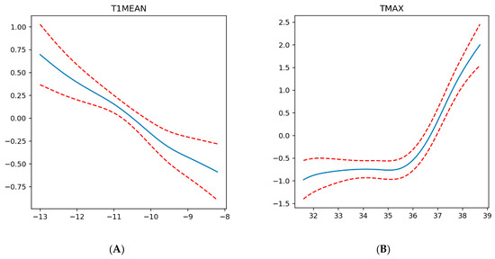
Figure 14.
Dependence of rill erosion density on temperature factors (°C)—mean annual temperature in January (A) and mean annual maximum temperature in the warm season (B).
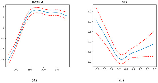
Figure 15.
Dependence of rill erosion density on mean annual precipitation in the warm period (mm) (A) and the value of the hydrothermal coefficient (GTK) (B) in the basin.
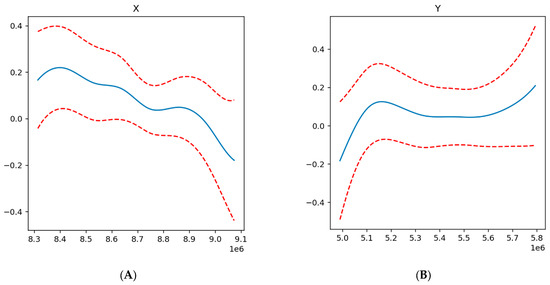
Figure 16.
Dependence of rill erosion density on geographical location: (A)—longitude (m), (B)—latitude (m).
Generalized models confirmed the known relationships between soil erosion and natural factors and revealed complex nonlinear relationships. It is observed that the density of the erosion network is stable with an increase in the average elevation of the basin, but up to 100 m, after which the growth of density is replaced by a decrease in the density and its stabilization (Figure 12A). In our opinion, this dependence should be considered in combination with the effect of average slope steepness on the density of the erosion network. In this case, the relationship is more superficial and closer to a direct linear relationship—the higher the steepness, the greater the density (Figure 12B). However, when analyzing steepness in basins with an average elevation of less than 100 m, a pattern becomes apparent—steepness does not exceed 3 degrees, and the slopes of these basins are well suited for farming, particularly as arable land. Indeed, in these areas, the percentage of the plowed area exceeds 50%.
The effect of relief morphometry is also confirmed by the dependence of the density of rill erosion on the height dispersion index in the basin—the difference between the maximum and minimum heights. In general, the smaller the height difference, the lower the density, but fundamentally, the most significant decrease in rill erosion intensity is observed in basins with a small height difference (up to ~70 m), after which the intensity of density reduction is not as pronounced and essentially remains constant (Figure 13A). The influence of anthropogenic development on the intensity of erosion processes is also confirmed by the inverse relationship between forest cover and the density of the rill network (Figure 13B).
Climatic factors have no less influence on the character of erosion processes in the study area, partly complementing the topographic and economic predisposition of the area to the development of rills. The relationship between the density of rill erosion and the average air temperature in January is interesting—the lower the mean annual temperature in the coldest month of the year, the more intense the process’s pattern is (Figure 14A). It seems to be related to the soil freezing capacity, which ensures the intensity of the erosion processes. However, it is impossible to verify this reliably due to the lack of adequate models of soil freezing in the study area. Temperature influences the character of erosion processes in summer as well—there is a strong direct correlation between the intensity of the process and the maximum air temperature starting from 36 degrees Celsius (Figure 14B). Initially, the authors attributed this to the potentially high evaporation capacity at such temperatures and the possible high precipitation intensity. However, analysis of the dependence of erosion processes on the precipitation layer in the warm season and the zoning map of the study area by the maximum temperature rejected this hypothesis. The maximum air temperatures are associated with erosion processes indirectly through the prevailing soil types, as the conditions for the emergence of one or another type. This is confirmed because the areas with maximum temperatures over 36 degrees are located in the transition zone of semi-deserts and dry-steppes with prevailing chestnut and solonetz soil types. These types of soils are characterized by a large number of cracks reaching a depth of 5–6 cm [80]. Even with an aggregate not large annual precipitation layer, the passing rains create a continuous surface runoff on the dry soils, which erodes the soils along the available cracks, forming stable washouts.
In general, the relationship between the intensity of rill erosion and moisture is direct; there is a steady trend to an increase in the density of the erosion network with increasing precipitation in the warm period up to ~270 mm, after which the role of precipitation decreases while maintaining the rule—“much precipitation—more intense erosion” (Figure 15A). Stabilization of the trend, in this case, is explained by the fact that 270 mm is a kind of boundary between steppe and forest-steppe zones, in which there is a clear seasonality of precipitation. By the time of the most intensive precipitation (summer-autumn period), vegetation with good soil-protective properties develops on these territories [24], which becomes the dominant factor of soil erosion intensification. The influence of moisture factors most clearly shows the relationship between the density of rill erosion and the value of the hydrothermal coefficient of the territory (Figure 15B). The density of the erosion network decreases with increasing GTK up to the value of 0.7—a clear border between arid area and wetted area. The intensity of soil-protecting vegetation increases with the increase of the SCC, but the precipitation becomes sufficient for the vegetation to perform its soil-protecting functions less effectively when moving into the wetted zone.
The analysis of the influence of the geographical location of the basin on the intensity of erosion processes also demonstrated statistically significant relationships. The density of rill erosion decreases linearly as one move to the east of the study area (Figure 16A), which is explained by the fact that the western part of the study area has a higher right bank of the Volga River and, as a result, higher values of slope steepness, which, as shown earlier, directly affect the intensity of the process. The latitudinal pattern is not so linear and more complex (Figure 16B)—with moving from the south to the north up to the zone of typical steppes, there is a systematic increase in the density of rill erosion, after which there is some decrease in the intensity of soil erosion and its stabilization, after which, starting from the northern part of the forest-steppe zone there is another gradual increase in the intensity of erosion activity. The reasons for this, as previously shown, lie in the zonal features of the study area, changes in the degree of moisture, as well as the types of plant communities, including agricultural ones, growing in a particular area.
It is worth separately considering the influence of soil-geological conditions of erosion processes. A one-factor analysis of variance was conducted to analyze the relationship between the prevailing soil type and total rill erosion length (Figure 17).
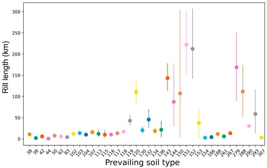
Figure 17.
Dependence of the length of the erosion network on the prevailing soil type. Soil types are given in the Supplementary Materials.
The basic soils of taiga and coniferous-broadleaved forests, as well as hydromorphic soils, are least susceptible to erosion activity. The smallest total length of rills is observed on sod-podzol soils (shallow-podzol and deep-podzol). These taiga soils, as a rule, are covered by mixed forests with a dense canopy and good protection against the formation of surface runoff. Moving southward, there is a slight increase in the total length of the rill network on gray forest soils of various subtypes. These soils are actively involved in agricultural management and have suitable hydrometeorological conditions. Weak susceptibility to erosion of territories with hydromorphic soils is, in our opinion, evident and connected, by and large, with land use on such soils—these are meadows with maximum soil-protective properties. The next group of soils is more affected by erosion processes—steppe soils. These are all kinds of chernozems, starting from leached chernozems. Southern chernozems, which are peculiar “record-breakers” by erosion susceptibility among typical steppes soils, are distinguished. Southern chernozems are in the cluster with the highest density of erosion network (Figure 7). Southern chernozems are spread in the southern part of the steppe zone. They are formed in the conditions of semiarid climate under soddy-cereal medium steppes. Grass cover is sparse, clearly expressed summer semi-rest period for most dominant cereals. Soil-forming rocks are represented mainly by loess and loess-like loams, often containing easily soluble salts, as well as eluvial-deluvial deposits. Water conditions of soils are solid. Agricultural development of southern chernozems is high: in the European part of Russia, it exceeds 50%, while moving to the east, plowing decreases and the number of pastures increases. The main crops grown are cereals (wheat and corn) and legumes; considerable areas are occupied by industrial crops (sugar beet and tobacco), vegetable, and melon crops. Plowed soils are prone to water and wind erosion, structural degradation, and slitization under irrigation. The last group is soils with a maximum total length of erosion network—soils of dry steppes and semi-deserts. These are different subtypes of chestnut soils and solonetz soils, a description of which was given earlier.
The one-factor analysis of variance was also applied to analyze the relationship between erosion activity and the predominant type of soil-forming rocks (Figure 18). In this case, grouping types is problematic due to implicit clustering; however, certain patterns are still observed. The increase in total length of rill erosion directly depends on clay content in the soil-forming rock and—in its water-holding capacity, drainability. The minimum, near-zero erosion network length is observed on weakly erodible shales. Analyzing the rocks on which erosion is observed, the minimum length of the erosion network falls on the group of rocks conditionally united into the so-called “sands”—these are sandy rocks and sandstones. These rocks have the maximum infiltration capacity, not allowing the formation of washout surface runoff and coming to the soils with minimal humus horizons. Slightly better eroded areas are composed of clayey and loamy rocks, underlain by sandy and sandy loam rocks, as well as light loam rocks themselves. Medium loamy rocks and rocks of different textures with a predominance of loam and clay are better eroded. On average, easily erodible chalky rocks—limestone and other carbonate rocks—are even better erodible. They usually form gray forest soils and leached chernozems, heavily involved in agricultural production. The most significant total length of the erosion network is expected to be in water-resistant clay and heavy loam rocks, on which surface runoff is formed, eroding fertile soil layers. Separately, sandy loam rocks, for which we could not find a reliable relationship—these rocks, draining well the surface runoff, can be resistant to erosion processes and, folding typical chernozems, due to active economic activity falls in the area of maximum rill erosion.
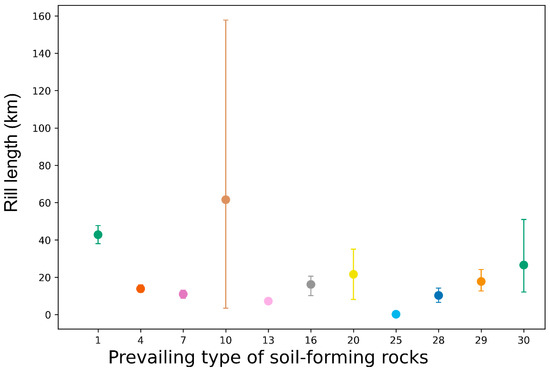
Figure 18.
Dependence of the length of the erosion network on the prevailing type of soil-forming rocks. The rock types are given in the Supplementary Materials.
The analysis of variance was conducted separately by landscape zones, and the result can be observed in Figure 19. The results confirm the earlier conclusions—the zones of dry and typical steppes and semi-deserts are most susceptible to erosion processes.
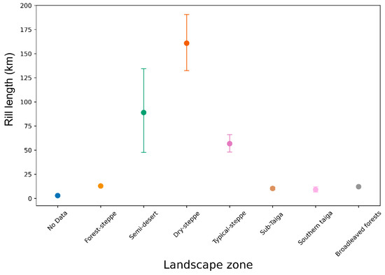
Figure 19.
Relationship between the rill erosion network length and landscape zone.
The analysis of the relationship between erosion processes and anthropogenic load also confirms the previous conclusions (Figure 20). The score of the anthropogenic load is given based on the development of the territory, the presence of settlements, industry, and roads of various types, as well as population density.
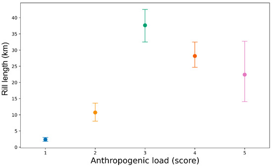
Figure 20.
The dependence of the length of the rill erosion network on the anthropogenic load.
The intensity of erosion processes increases with increasing anthropogenic load, but not linearly. The maximum intensity of erosion is observed under moderate anthropogenic load. Decrease of the total length of erosion forms with further increase of anthropogenic load is related to decrease of the area not occupied by cities, manufactories, and other anthropogenic objects.
The cumulative effect of anthropogenic load, forest cover, prevailing soil type, and soil-forming rocks has the most significant contribution to the development of erosion processes in the study area (Figure 21).
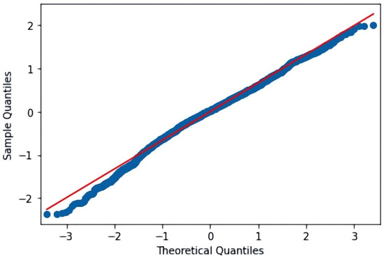
Figure 21.
QQ–plot of MANOVA between rill network and forest cover, anthropogenic load, prevailing soil type, and soil-forming rocks.
5. Conclusions
Deep neural networks can effectively solve geomorphological problems, allowing large-scale mapping of erosion processes. For the first time in the world, a detailed assessment of the density of rill erosion and its relation to the main natural–anthropogenic factors is given. In this case, preparation of the training sample is the most time-consuming stage, taking 2/3 of the whole time of the study. The trained model allows highly efficient and at an acceptable level of recognition of the erosion network on high-resolution images, in our case using Sentinel-2 images. We investigated which Sentinel-2 bands allow the most efficient visual recognition at the preliminary stage. As a result of numerous experiments, the best “readability” of the image was demonstrated by a separate near-infrared band, winning in comparison with RGB-synthesis, synthesis of artificial colors in various combinations, and other channels, separately. Another sensitive point of the research is the choice of neural network architecture for semantic segmentation. Experiments were carried out with the most common architectures for such tasks, including the well-known U-Net architecture, as well as FPN, PSPNet, and LinkNet in combination with the most popular encoder groups, such as VGG, ResNet, SE-ResNet, ResNeXt, SE-ResNeXt, SENet154, DenseNet, Inception, MobileNet, and EfficientNet. The best recognition accuracy on the test set showed the FPN + EfficientNet combination; however, when applying the trained model, the recognition results were poor. The best results in terms of real-world applications were achieved using LinkNet + DenseNet (DenseNet201). In the future, it is planned to use the trained model to recognize the erosion network for 2019–2020 to assess the dynamics of erosion processes in time.
The analysis made it possible to assess the key factors influencing the intensity of rill erosion processes at a high level of confidence. In some cases, existing knowledge about the influence of certain factors on soil erosion was confirmed. Particular interest is the possibility of mapping the territories with the highest risk of erosion processes due to natural–anthropogenic conditions, which will allow producing precise and effective measures to minimize the risks. Under the conditions of intensive agricultural development, no reduction of anthropogenic load can be discussed; however, proper crop rotations, regular sowing of perennial grasses, and proper plowing will reduce the existing risks many times.
The use of generalized additive models (GAM) to analyze dependencies made it possible to describe complex relationships between the density of rill erosion and climate, geomorphological, and other geographic factors. Unfortunately, not all parameters could be used in the analysis; in the future, detailed modeling of the dependence of erosion processes on factors of soil freezing, and the intensity of precipitation, especially changes in intensity in time series, should be conducted.
Supplementary Materials
The following supporting information can be downloaded at: https://www.mdpi.com/article/10.3390/ijgi11030197/s1, Table S1: Prevailing soil type list; Table S2: Prevailing type of soil-forming rocks list.
Funding
This research was funded by grant number MK-2005.2021.1.5.
Institutional Review Board Statement
Not applicable.
Informed Consent Statement
Not applicable.
Data Availability Statement
The data presented in this study are available on request from the corresponding author and partially available on the http://bassepr.kpfu.ru/ accessed on 15 December 2021.
Acknowledgments
The author would like to thank Yandex Cloud (https://cloud.yandex.com/ accessed on 30 December 2021) for providing computing resources for the project within the Yandex Datasphere product. The author would like to thank the reviewers for their helpful comments and suggestions, which improved the manuscript.
Conflicts of Interest
The authors declare no conflict of interest.
References
- Yang, Y.; Shi, Y.; Liang, X.; Huang, T.; Fu, S.; Liu, B. Evaluation of Structure from Motion (SfM) Photogrammetry on the Measurement of Rill and Interrill Erosion in a Typical Loess. Geomorphology 2021, 385, 107734. [Google Scholar] [CrossRef]
- Di Stefano, C.; Ferro, V.; Pampalone, V.; Sanzone, F. Field Investigation of Rill and Ephemeral Gully Erosion in the Sparacia Experimental Area, South Italy. Catena 2013, 101, 226–234. [Google Scholar] [CrossRef]
- Murgatroyd, A.L.; Ternan, J.L. The Impact of Afforestation on Stream Bank Erosion and Channel Form. Earth Surf. Process. Landf. 1983, 8, 357–369. [Google Scholar] [CrossRef]
- Nearing, M.A.; Norton, L.D.; Bulgakov, D.A.; Larionov, G.A.; West, L.T.; Dontsova, K.M. Hydraulics and Erosion in Eroding Rills. Water Resour. Res. 1997, 33, 865–876. [Google Scholar] [CrossRef]
- Yermolaev, O.P.; Gafurov, A.M.; Usmanov, B.M. Evaluation of Erosion Intensity and Dynamics Using Terrestrial Laser Scanning. Eurasian Soil Sci. 2018, 51, 814–826. [Google Scholar] [CrossRef]
- Kociuba, W.; Janicki, G.; Rodzik, J.; Stępniewski, K. Comparison of Volumetric and Remote Sensing Methods (TLS) for Assessing the Development of a Permanent Forested Loess Gully. Nat. Hazards 2015, 79, 139–158. [Google Scholar] [CrossRef]
- Vinci, A.; Brigante, R.; Todisco, F.; Mannocchi, F.; Radicioni, F. Measuring Rill Erosion by Laser Scanning. Catena 2015, 124, 97–108. [Google Scholar] [CrossRef]
- Usmanov, B.; Yermolaev, O.; Gafurov, A. Estimates of Slope Erosion Intensity Utilizing Terrestrial Laser Scanning. Proc. Int. Assoc. Hydrol. Sci. 2015, 367, 59–65. [Google Scholar] [CrossRef]
- Hu, T.; Sun, X.; Su, Y.; Guan, H.; Sun, Q.; Kelly, M.; Guo, Q. Development and Performance Evaluation of a Very Low-Cost UAV-Lidar System for Forestry Applications. Remote Sens. 2021, 13, 77. [Google Scholar] [CrossRef]
- Nex, F.; Remondino, F. UAV for 3D Mapping Applications: A Review. Appl. Geomat. 2014, 6, 1–15. [Google Scholar] [CrossRef]
- Gafurov, A.M. Possible Use of Unmanned Aerial Vehicle for Soil Erosion Assessment. Uchenye Zap. Kazan. Univ. Ser. Estestv. Nauk. 2017, 159, 654–667. [Google Scholar]
- Gafurov, A. The Methodological Aspects of Constructing a High-Resolution DEM of Large Territories Using Low-Cost UAVs on the Example of the Sarycum Aeolian Complex, Dagestan, Russia. Drones 2021, 5, 7. [Google Scholar] [CrossRef]
- Pandey, A.; Himanshu, S.K.; Mishra, S.K.; Singh, V.P. Physically Based Soil Erosion and Sediment Yield Models Revisited. Catena 2016, 147, 595–620. [Google Scholar] [CrossRef]
- Wischmeier, W.H.; Smith, D.D. Predicting Rainfall Erosion Losses-a Guide to Conservation Planning; U.S. Department of Agriculture: Betsville, MD, USA, 1978.
- Renard, K.G.; Foster, G.R.; Weesies, G.A.; Porter, J.P. RUSLE: Revised Universal Soil Loss Equation. J. Soil Water Conserv. 1991, 46, 30–33. [Google Scholar]
- Sadeghi, S.H.R.; Gholami, L.; Darvishan, A.K.; Saeidi, P. A Review of the Application of the MUSLE Model Worldwide. Hydrol. Sci. J. 2014, 59, 365–375. [Google Scholar] [CrossRef] [Green Version]
- Knisel, W.G. CREAMS: A Field Scale Model for Chemicals, Runoff, and Erosion from Agricultural Management Systems; Department of Agriculture, Science and Education Administration: Baltimore, MD, USA, 1980. [Google Scholar]
- De Roo, A.P.J.; Wesseling, C.G.; Jetten, V.G.; Ritsema, C. LISEM: A Physically-Based Hydrological and Soil Erosion Model Incorporated in a GIS. In Application of Geographic Information Systems in Hydrology and Water Resources Management; Kovar, K., Nachtnebel, H.P., Eds.; IAHS: Wallingford, UK, 1996; Volume 235, pp. 395–403. [Google Scholar]
- Flanagan, D.C.; Ascough, J.C.; Nearing, M.A.; Laflen, J.M. The Water Erosion Prediction Project (WEPP) Model. In Landscape Erosion and Evolution Modeling; Harmon, R.S., Doe, W.W., Eds.; Springer: Boston, MA, USA, 2001; pp. 145–199. ISBN 978-1-4615-0575-4. [Google Scholar]
- Favis-Mortlock, D.T.; Boardman, J.; Parsons, A.J.; Lascelles, B. Emergence and Erosion: A Model for Rill Initiation and Development. Hydrol. Process. 2000, 14, 2173–2205. [Google Scholar] [CrossRef]
- Misra, R.K.; Rose, C.W. Application and Sensitivity Analysis of Process-Based Erosion Model GUEST. Eur. J. Soil Sci. 1996, 47, 593–604. [Google Scholar] [CrossRef]
- Mahmoodabadi, M.; Ghadiri, H.; Rose, C.; Yu, B.; Rafahi, H.; Rouhipour, H. Evaluation of GUEST and WEPP with a New Approach for the Determination of Sediment Transport Capacity. J. Hydrol. 2014, 513, 413–421. [Google Scholar] [CrossRef]
- Morgan, R.P.C.; Quinton, J.N.; Smith, R.E.; Govers, G.; Poesen, J.W.A.; Auerswald, K.; Chisci, G.; Torri, D.; Styczen, M.E. The European Soil Erosion Model (EUROSEM): A Dynamic Approach for Predicting Sediment Transport from Fields and Small Catchments. Earth Surf. Process. Landf. 1998, 23, 527–544. [Google Scholar] [CrossRef]
- Mukharamova, S.; Saveliev, A.; Ivanov, M.; Gafurov, A.; Yermolaev, O. Estimating the Soil Erosion Cover-Management Factor at the European Part of Russia. ISPRS Int. J. Geo-Inf. 2021, 10, 645. [Google Scholar] [CrossRef]
- Maltsev, K.A.; Golosov, V.N.; Gafurov, A.M. Digital Elevation Models and Their Use for Assessing Soil Erosion Rates on Arable Lands. Uchenye Zap. Kazan. Universiteta Seriya Estestv. Nauk. 2018, 160, 514–530. [Google Scholar]
- Pielke, R.A.; Cotton, W.R.; Walko, R.L.; Tremback, C.J.; Lyons, W.A.; Grasso, L.D.; Nicholls, M.E.; Moran, M.D.; Wesley, D.A.; Lee, T.J.; et al. A Comprehensive Meteorological Modeling System—RAMS. Meteorol. Atmos. Phys. 1992, 49, 69–91. [Google Scholar] [CrossRef]
- Sheffield, J.; Goteti, G.; Wood, E.F. Development of a 50-Year High-Resolution Global Dataset of Meteorological Forcings for Land Surface Modeling. J. Clim. 2006, 19, 3088–3111. [Google Scholar] [CrossRef] [Green Version]
- Shruthi, R.B.V.; Kerle, N.; Jetten, V. Object-Based Gully Feature Extraction Using High Spatial Resolution Imagery. Geomorphology 2011, 134, 260–268. [Google Scholar] [CrossRef]
- Conoscenti, C.; Angileri, S.; Cappadonia, C.; Rotigliano, E.; Agnesi, V.; Märker, M. Gully Erosion Susceptibility Assessment by Means of GIS-Based Logistic Regression: A Case of Sicily (Italy). Geomorphology 2014, 204, 399–411. [Google Scholar] [CrossRef] [Green Version]
- Conoscenti, C.; Agnesi, V.; Cama, M.; Caraballo-Arias, N.A.; Rotigliano, E. Assessment of Gully Erosion Susceptibility Using Multivariate Adaptive Regression Splines and Accounting for Terrain Connectivity. Land Degrad. Dev. 2018, 29, 724–736. [Google Scholar] [CrossRef]
- Golosov, V.; Gusarov, A.; Sharifillin, A.; Ivanova, N.N.; Gafurov, A.; Yermolaev, O.; Rysin, I. Using Bomb-Derived and Chernobyl-Derived 137Cs for the Assessment of Soil Losses Trends in Different Landscape Zones of the European Russia. In Proceedings of the 14th International Symposium on the Interaction between Sediments and Water, Taormina, Italy, 17–22 June 2017; p. 10. [Google Scholar]
- Gusarov, A.V.; Golosov, V.N.; Sharifullin, A.G.; Gafurov, A.M. Contemporary Trend in Erosion of Arable Southern Chernozems (Haplic Chernozems Pachic) in the West of Orenburg Oblast (Russia). Eurasian Soil Sci. 2018, 51, 561–575. [Google Scholar] [CrossRef]
- Golosov, V.; Koiter, A.; Ivanov, M.; Maltsev, K.; Gusarov, A.; Sharifullin, A.; Radchenko, I. Assessment of Soil Erosion Rate Trends in Two Agricultural Regions of European Russia for the Last 60 Years. J. Soils Sediments 2018, 18, 3388–3403. [Google Scholar] [CrossRef]
- Gafurov, A.M. Using Unmanned Aerial Vehicles for Evaluation of Soil Erosion. Belgorod State Univ. Sci. Bull. Nat. Sci. 2019, 43, 182–190. [Google Scholar] [CrossRef]
- Yermolaev, O.P.; Medvedeva, R.A.; Platoncheva, E.V. Methodological Approaches to Monitoring Erosion of Agricultural Lands in the European Part of Russia by Using Satellite Imagery. Uchenye Zap. Kazan. Univ. Ser. Estestv. Nauk. 2017, 159, 668–680. [Google Scholar]
- Yermolayev, O.; Platoncheva, E.; Essuman-Quainoo, B. Spatial-Temporal Dynamics of the Ephemeral Gully Belt on the Plowed Slopes of River Basins in Natural and Anthropogenic Landscapes of the East of the Russian Plain. Geosciences 2020, 10, 167. [Google Scholar] [CrossRef]
- Seutloali, K.E.; Dube, T.; Mutanga, O. Assessing and Mapping the Severity of Soil Erosion Using the 30-m Landsat Multispectral Satellite Data in the Former South African Homelands of Transkei. Phys. Chem. Earth Parts A/B/C 2017, 100, 296–304. [Google Scholar] [CrossRef]
- Saadat, H.; Adamowski, J.; Tayefi, V.; Namdar, M.; Sharifi, F.; Ale-Ebrahim, S. A New Approach for Regional Scale Interrill and Rill Erosion Intensity Mapping Using Brightness Index Assessments from Medium Resolution Satellite Images. Catena 2014, 113, 306–313. [Google Scholar] [CrossRef]
- Desprats, J.F.; Raclot, D.; Rousseau, M.; Cerdan, O.; Garcin, M.; Le Bissonnais, Y.; Ben Slimane, A.; Fouche, J.; Monfort-Climent, D. Mapping Linear Erosion Features Using High and Very High Resolution Satellite Imagery. Land Degrad. Dev. 2013, 24, 22–32. [Google Scholar] [CrossRef]
- Fiorucci, F.; Ardizzone, F.; Rossi, M.; Torri, D. The Use of Stereoscopic Satellite Images to Map Rills and Ephemeral Gullies. Remote Sens. 2015, 7, 14151–14178. [Google Scholar] [CrossRef] [Green Version]
- Kashtanov, A.N.; Vernyuk, Y.I.; Savin, I.Y.; Shchepot’ev, V.V.; Dokukin, P.A.; Sharychev, D.V.; Li, K.A. Mapping of Rill Erosion of Arable Soils Based on Unmanned Aerial Vehicles Survey. Eurasian Soil Sci. 2018, 51, 479–484. [Google Scholar] [CrossRef]
- Karydas, C.; Bouarour, O.; Zdruli, P. Mapping Spatio-Temporal Soil Erosion Patterns in the Candelaro River Basin, Italy, Using the G2 Model with Sentinel2 Imagery. Geosciences 2020, 10, 89. [Google Scholar] [CrossRef] [Green Version]
- Walter, V. Object-Based Classification of Remote Sensing Data for Change Detection. ISPRS J. Photogramm. Remote Sens. 2004, 58, 225–238. [Google Scholar] [CrossRef]
- Zhang, F.; Li, J.; Zhang, B.; Shen, Q.; Ye, H.; Wang, S.; Lu, Z. A Simple Automated Dynamic Threshold Extraction Method for the Classification of Large Water Bodies from Landsat-8 OLI Water Index Images. Int. J. Remote Sens. 2018, 39, 3429–3451. [Google Scholar] [CrossRef]
- Ghosh, A.; Maiti, R. Soil Erosion Susceptibility Assessment Using Logistic Regression, Decision Tree and Random Forest: Study on the Mayurakshi River Basin of Eastern India. Environ. Earth Sci. 2021, 80, 328. [Google Scholar] [CrossRef]
- Dinh, T.V.; Nguyen, H.; Tran, X.-L.; Hoang, N.-D. Predicting Rainfall-Induced Soil Erosion Based on a Hybridization of Adaptive Differential Evolution and Support Vector Machine Classification. Math. Probl. Eng. 2021, 2021, e6647829. [Google Scholar] [CrossRef]
- Liu, Y.; Zhou, J.; Qi, W.; Li, X.; Gross, L.; Shao, Q.; Zhao, Z.; Ni, L.; Fan, X.; Li, Z. ARC-Net: An Efficient Network for Building Extraction from High-Resolution Aerial Images. IEEE Access 2020, 8, 154997–155010. [Google Scholar] [CrossRef]
- Cai, J.; Chen, Y. MHA-Net: Multipath Hybrid Attention Network for Building Footprint Extraction from High-Resolution Remote Sensing Imagery. IEEE J. Sel. Top. Appl. Earth Obs. Remote Sens. 2021, 14, 5807–5817. [Google Scholar] [CrossRef]
- Luo, L.; Li, P.; Yan, X. Deep Learning-Based Building Extraction from Remote Sensing Images: A Comprehensive Review. Energies 2021, 14, 7982. [Google Scholar] [CrossRef]
- Blais, M.-A.; Akhloufi, M.A. Deep Learning for Low Altitude Coastline Segmentation; Online Only; SPIE: Orlando, FL, USA, 2021; Volume 11752. [Google Scholar]
- Aryal, B.; Escarzaga, S.M.; Vargas Zesati, S.A.; Velez-Reyes, M.; Fuentes, O.; Tweedie, C. Semi-Automated Semantic Segmentation of Arctic Shorelines Using Very High-Resolution Airborne Imagery, Spectral Indices and Weakly Supervised Machine Learning Approaches. Remote Sens. 2021, 13, 4572. [Google Scholar] [CrossRef]
- Garg, R.; Kumar, A.; Bansal, N.; Prateek, M.; Kumar, S. Semantic Segmentation of PolSAR Image Data Using Advanced Deep Learning Model. Sci. Rep. 2021, 11, 15365. [Google Scholar] [CrossRef]
- Dong, Y.; Li, F.; Hong, W.; Zhou, X.; Ren, H. Land Cover Semantic Segmentation of Port Area with High Resolution SAR Images Based on SegNet. In 2021 SAR in Big Data Era (BIGSARDATA); Institute of Electrical and Electronics Engineers (IEEE): Piscataway, NJ, USA, 2021; pp. 1–4. [Google Scholar] [CrossRef]
- Wei, H.; Xu, X.; Ou, N.; Zhang, X.; Dai, Y. Deanet: Dual Encoder with Attention Network for Semantic Segmentation of Remote Sensing Imagery. Remote Sens. 2021, 13, 3900. [Google Scholar] [CrossRef]
- Illarionova, S.; Trekin, A.; Ignatiev, V.; Oseledets, I. Tree Species Mapping on Sentinel-2 Satellite Imagery with Weakly Supervised Classification and Object-Wise Sampling. Forests 2021, 12, 1413. [Google Scholar] [CrossRef]
- Song, G.; Wu, S.; Lee, C.K.F.; Serbin, S.P.; Wolfe, B.T.; Ng, M.K.; Ely, K.S.; Bogonovich, M.; Wang, J.; Lin, Z.; et al. Monitoring Leaf Phenology in Moist Tropical Forests by Applying a Superpixel-Based Deep Learning Method to Time-Series Images of Tree Canopies. ISPRS J. Photogramm. Remote Sens. 2022, 183, 19–33. [Google Scholar] [CrossRef]
- Gafurov, A.M.; Yermolayev, O.P. Automatic Gully Detection: Neural Networks and Computer Vision. Remote Sens. 2020, 12, 1743. [Google Scholar] [CrossRef]
- Du, B.; Zhao, Z.; Hu, X.; Wu, G.; Han, L.; Sun, L.; Gao, Q. Landslide Susceptibility Prediction Based on Image Semantic Segmentation. Comput. Geosci. 2021, 155, 104860. [Google Scholar] [CrossRef]
- Yermolaev, O.; Usmanov, B.; Gafurov, A.; Poesen, J.; Vedeneeva, E.; Lisetskii, F.; Nicu, I.C. Assessment of Shoreline Transformation Rates and Landslide Monitoring on the Bank of Kuibyshev Reservoir (Russia) Using Multi-Source Data. Remote Sens. 2021, 13, 4214. [Google Scholar] [CrossRef]
- Yermolaev, O.P.; Mukharamova, S.S.; Maltsev, K.A.; Ivanov, M.A.; Ermolaeva, P.O.; Gayazov, A.I.; Mozzherin, V.V.; Kharchenko, S.V.; Marinina, O.A.; Lisetskii, F.N. Geographic Information System and Geoportal «River Basins of the European Russia». IOP Conf. Ser. Earth Environ. Sci. 2018, 107, 012108. [Google Scholar] [CrossRef]
- Gafurov, A.M.; Rysin, I.I.; Golosov, V.N.; Grigoryev, I.I.; Sharifullin, A.G. Estimation of the recent rate of gully head retreat on the southern megaslope of the East European Plain using a set of instrumental methods. Vestn. Mosk. Univ. Seriya 5 Geogr. 2018, 2018, 61–71. [Google Scholar]
- Gorelick, N.; Hancher, M.; Dixon, M.; Ilyushchenko, S.; Thau, D.; Moore, R. Google Earth Engine: Planetary-Scale Geospatial Analysis for Everyone. Remote Sens. Environ. 2017, 202, 18–27. [Google Scholar] [CrossRef]
- Ke, G.; Meng, Q.; Finley, T.; Wang, T.; Chen, W.; Ma, W.; Ye, Q.; Liu, T.-Y. LightGBM: A Highly Efficient Gradient Boosting Decision Tree. In Advances in Neural Information Processing Systems 30 (NIPS 2017); Curran Associates, Inc.: Long Beach, CA, USA, 2017; Volume 30. [Google Scholar]
- Chaurasia, A.; Culurciello, E. LinkNet: Exploiting Encoder Representations for Efficient Semantic Segmentation. In Proceedings of the 2017 IEEE Visual Communications and Image Processing (VCIP), St. Petersburg, FL, USA, 10–13 December 2017; pp. 1–4. [Google Scholar]
- Ronneberger, O.; Fischer, P.; Brox, T. U-Net: Convolutional Networks for Biomedical Image Segmentation. arXiv 2015, arXiv:1505.04597. [Google Scholar]
- Iandola, F.; Moskewicz, M.; Karayev, S.; Girshick, R.; Darrell, T.; Keutzer, K. DenseNet: Implementing Efficient ConvNet Descriptor Pyramids. arXiv 2014, arXiv:1404.1869. [Google Scholar]
- Jaccard, P. The Distribution of the Flora in the Alpine Zone. New Phytol. 1912, 11, 37–50. [Google Scholar] [CrossRef]
- Miller, R.G., Jr. Beyond ANOVA: Basics of Applied Statistics; CRC Press: Boca Raton, FL, USA, 1997; ISBN 978-0-412-07011-2. [Google Scholar]
- Huberty, C.J.; Olejnik, S. Applied MANOVA and Discriminant Analysis; John Wiley & Sons: Hoboken, NJ, USA, 2006; ISBN 978-0-471-78946-8. [Google Scholar]
- Groisman, P.Y.A.; Karl, T.R.; Easterling, D.R.; Knight, R.W.; Jamason, P.F.; Hennessy, K.J.; Suppiah, R.; Page, C.M.; Wibig, J.; Fortuniak, K.; et al. Changes in the probability of heavy precipitation: Important indicators of climatic change. In Weather and Climate Extremes; Karl, T.R., Nicholls, N., Ghazi, A., Eds.; Springer: Dordrecht, The Netherlands, 1999; pp. 243–283. ISBN 978-90-481-5223-0. [Google Scholar]
- Dore, M.H.I. Climate Change and Changes in Global Precipitation Patterns: What Do We Know? Environ. Int. 2005, 31, 1167–1181. [Google Scholar] [CrossRef]
- Zolina, O.; Simmer, C.; Gulev, S.K.; Kollet, S. Changing Structure of European Precipitation: Longer Wet Periods Leading to More Abundant Rainfalls: Changing Structure of European Rainfall. Geophys. Res. Lett. 2010, 37, 1–5. [Google Scholar] [CrossRef]
- Olchev, A.; Novenko, E.; Popov, V.; Pampura, T.; Meili, M. Evidence of Temperature and Precipitation Change over the Past 100 Years in a High-Resolution Pollen Record from the Boreal Forest of Central European Russia. Holocene 2017, 27, 740–751. [Google Scholar] [CrossRef]
- Zolotokrylin, A.; Cherenkova, E. Seasonal Changes in Precipitation Extremes in Russia for the Last Several Decades and Their Impact on Vital Activities of the Human Population. Geogr. Environ. Sustain. 2017, 10, 69–82. [Google Scholar] [CrossRef] [Green Version]
- Golosov, V.; Gusarov, A.; Litvin, L.; Yermolaev, O.; Chizhikova, N.; Safina, G.; Kiryukhina, Z. Evaluation of Soil Erosion Rates in the Southern Half of the Russian Plain: Methodology and Initial Results. Proc. Int. Assoc. Hydrol. Sci. 2017, 375, 23–27. [Google Scholar] [CrossRef]
- Sharifullin, A.; Gusarov, A.; Gafurov, A.; Essuman-Quainoo, B. Preliminary Estimating the Contemporary Sedimentation Trend in Dry Valley Bottoms of First-Order Catchments of Different Landscape Zones of the Russian Plain Using the 137CS as a Chronomarker. IOP Conf. Ser. Earth Environ. Sci. 2018, 107, 012022. [Google Scholar] [CrossRef]
- Hastie, T.; Tibshirani, R. Generalized Additive Models; Chapman & Hall/CRC: Boca Raton, FL, USA, 1999; ISBN 978-0-412-34390-2. [Google Scholar]
- Yermolaev, O.; Mukharamova, S.; Vedeneeva, E. River Runoff Modeling in the European Territory of Russia. Catena 2021, 203, 105327. [Google Scholar] [CrossRef]
- Servén, D.; Brummitt, C.; Abedi, H. Hlink Dswah/Pygam: V0.8.0; Zenodo: Genève, Switzerland, 2018. [Google Scholar]
- Babayan, L.A.; Protopopov, V.M. The Fertility of Light Chestnut Soils on Different Elements of Watershed Topography. Eurasian Soil Sci. 1997, 30, 1113–1116. [Google Scholar]
Publisher’s Note: MDPI stays neutral with regard to jurisdictional claims in published maps and institutional affiliations. |
© 2022 by the author. Licensee MDPI, Basel, Switzerland. This article is an open access article distributed under the terms and conditions of the Creative Commons Attribution (CC BY) license (https://creativecommons.org/licenses/by/4.0/).