Modeling the Spatial and Temporal Spread of COVID-19 in Poland Based on a Spatial Interaction Model

Abstract

This article describes an original methodology for integrating global SIR-like epidemic models with spatial interaction models, which enables the forecasting of COVID-19 dynamics in Poland through time and space. Mobility level, estimated by the regional population density and distances among inhabitants, was the determining variable in the spatial interaction model. The spatiotemporal diffusion model, which allows the temporal prediction of case counts and the possibility of determining their spatial distribution, made it possible to forecast the dynamics of the COVID-19 pandemic at a regional level in Poland. This model was used to predict incidence in 380 counties in Poland, which represents a much more detailed modeling than NUTS 3 according to the widely used geocoding standard Nomenclature of Territorial Units for Statistics. The research covered the entire territory of Poland in seven weeks of early 2021, just before the start of vaccination in Poland. The results were verified using official epidemiological data collected by sanitary and epidemiological stations. As the conducted analyses show, the application of the approach proposed in the article, integrating epidemiological models with spatial interaction models, especially unconstrained gravity models and destination (attraction) constrained models, leads to obtaining almost 90% of the coefficient of determination, which reflects the quality of the model’s fit with the spatiotemporal distribution of the validation data.

1. Introduction

COVID-19 is an infectious disease caused by the newly discovered coronavirus, SARS-CoV-2. The virus was first discovered in Wuhan, China, and has quickly spread all around the world, infecting populations in most countries. The spread of COVID-19 is inherently a spatial process; therefore, attempts to combat its spread would benefit from modeling spatial interactions. This article expands on a previous study using gravity models to model the spatial development of the COVID-19 pandemic in Poland [1]. The present study describes the parameterization method of epidemiological models, and the development of spatial interaction models to simulate the pandemic development and determine the spatial (and temporal) distribution of the number of cases in Poland. Reference data on the number of cases in individual powiats (county-level administrative districts) provided by sanitary and epidemiological stations have confirmed the reliability of the prediction. However, the complexity of factors influencing the dissemination of SARS-CoV-2 poses a challenge, as it is extremely difficult to understand the relationships between individual variables and the outcomes being measured. Despite similarities to past respiratory viral illnesses such as SARS and MERS, as well as to annual seasonal influenza, COVID-19 has specific characteristics including heightened transmissibility [2,3]. It should also be noted that international traffic and tourism strongly increased the spread of the disease, globally, when compared with the viral diseases mentioned above. The relatively high infectivity and long incubation period, and the long viral shedding period, have contributed to a high number of transmissions, many of which have occurred through human-to-human contact with individuals showing no or mild symptoms [4,5,6]. These features of COVID-19 make it more difficult to model its spread simultaneously in different spatial locations than to calculate the number of cases for the whole country.

Classical approaches to mathematical modeling of the spread of diseases, from the Kermack-McKendrick epidemic (compartmental) model to newer network models, as well as the family of stochastic models [7], assume mixing across the entire population without considering its diversity, variegation, and substratification. On the other hand, the literature on epidemic research presents numerous methods and models concerning morbidity and the spatial aspects of diseases. Frequentist approaches use cellular automata and multiagent simulations ([multi-]agent-based modeling), which appropriately reflect direct contacts among people. However, these approaches involve modeling each individual and are limited by computational burden. It is clear that concentrating on spatially distributed subpopulations may allow for more accurate modeling than perfect mixing models, while incurring a lower computational burden than, for instance, multiagent models.

Wilson [8] originally formulated a group of spatial interaction models in the context of urban and regional systems, but also proved their suitability as models of epidemics in complex spatial systems with mutual interactions [9]. The family of gravity models also became used in infectious disease epidemiology [10,11,12].

Whereas the gravity model concerns a pair of points, Stewart [13] introduced the notion of potential that encompasses the influence of all other points on a particular point [14]. The potential is a measure of the influence of the population size, referred to elsewhere in the paper as the mass m, located at some point (e.g., in the middle of a certain city/region) within a distance d from this point. The notion of population potential was used as a measure of the number of contacts between people [15], additionally taking into account the ‘first law of geography’ [16]. This approach is also used to model infectious diseases and epidemics [17]. Wilson [9] introduced the concept of the probability of such contacts into spatial interaction modeling, taking into account the spatial dimension (distance or its functional measure, e.g., time). This approach also uses the entropy measure, which is used to assess the quality of the model fit. In recent literature, several spatiotemporal models have been proposed for COVID-19. In most of them [18,19,20], interactions between countries are related to fluxes of people moving between locations. This leads to asymmetries that cannot be directly explained with the physical distance between two places. One such successful approach for modeling COVID-19 has been the SIDARTHE model [21].

Construed spatial global, national, and regional models of the pandemic have aimed to identify and monitor spatial and temporal patterns and trends, and further, to reach a better understanding of the relationship between different potential variables (environmental, socioeconomic, demographic, etc.), among other goals. Geographical information systems (GIS) play a pivotal role in understanding the spatial clustering, transmission trend, and mapping the spread of infectious diseases. Different GIS techniques have been fundamental to decision-making by authorities during the COVID-19 pandemic. They may also contribute significantly to organizational security in the post-pandemic period. A range of GIS models and applications for tracking the COVID-19 epidemic and factors influencing the spread of COVID-19 have been developed to date [22,23,24,25,26,27].

Despite similarities to other respiratory virus outbreaks, COVID-19 stands out in terms of its global scale and high infection rate. A comparison between the SARS outbreak in 2003 in China, caused by a similar coronavirus, and COVID-19, highlighted that COVID-19 is far more transmissible, spreading from a single city to the entire country in just 30 days [28]. The causes of this difference are thought to be manifold and may include social and demographic factors, local government containment strategies, and differences in the dynamics of transmission between these two coronaviruses [29]. There have been many attempts to build multivariate regression models to explain the number of cases in each county in ongoing studies. Population density, road network density, industrial and residential buildings, have been among the independent variables studied in such models. Typically, three groups of risk factors that shape the volume, intensity and spatial dispersion of diseases are taken into account when creating models: individual risk, natural environment (climatic) risk, and social and demographic risk. However, there is no convincing evidence regarding the rank-order of which factors are most important.

The aim of this study was to construct a model of the geographic dissemination of COVID-19 in Poland based on spatial interaction models. We put forward the research hypothesis that it is possible to achieve a good-quality model, assuming a single independent variable: the mass of the population in administrative units. This approach allows for synergies between the models, enabling the time forecast of case counts (e.g., the classical SIR epidemiological model) and models of spatial interactions. The combined application of these approaches enables a reliable prediction of the number of infected people in administrative divisions. Our model is intended as a support tool that includes a geographic spread to the conceptualization of disease spread. It could be used as an a priori tool for estimating the spatial locations of infection outbreaks, as well as a way of evaluating future infection rates. An important advantage of the constructed model is its spatial aspect; i.e., it enables the evaluation of the potential spatial differentiation of the infected number of people within the set of observed spatial units (for instance, counties in Poland), which is especially important in the case of COVID-19 and similar diseases.

This approach provides useful insights simulating spatial networks in a flexible way, reducing the burden of individual simulations and predictions for each individual–level observation. While it represents a simplification of the spatial spread of the infection of pandemics, it nevertheless provides the possibility to extend into metapopulation models and spatial numerical simulations of epidemics in complex networks [30,31]. In this way, models can include distances. All types of pre-existing mathematical models can be expanded to be solved, maximized, or estimated using the adopted spatial analysis approach, reducing the uncertainty of empirical data [32].

2. Methods

2.1. SIR and SIR-F Models

Well-known deterministic compartment susceptible–infected–recovered [33] epidemic models based on viral transmission (in this case SARS-CoV-2) within a population (N) have been used since the beginning of the 20th century, and are described using a set of ODE (ordinary differential) equations:

$$\frac{dS}{dt}=-\beta SI,\hspace{1em}\hspace{1em}\frac{dI}{dt}=\beta SI-\gamma I,\hspace{1em}\hspace{1em}\frac{dR}{dt}=\gamma I$$

(1)

S + I + R = N   for all t

(2)

where S, I, and R are the numbers of susceptible, infected, and recovered individuals, respectively; N is the size of the population; $\beta$ is the contact rate capturing the ‘interaction frequency’, the rate of flow from susceptible to infected; $\gamma$ is the recovery rate, the rate of flow from infected to recovered or dead; and t denotes time [34]. There are several variations of models derived from the basic SIR model. In this paper, we apply the SIR-F model, which partitions the R (recovered) population into recovered and failed (deceased) subpopulations.

2.2. Gravity Model

The general formula of population gravity between two certain points is described as T_ij = f (O_i,D_j, d_ij), where T_ij is the volume of interactions (contacts), O_i is the flow emanating from the origin i and representing the push factor (e.g., emissiveness), D_j is the flow terminating at the destination point j and representing the pull factor (e.g., attraction), and d_ij is the distance between i and j representing the spatial separation (e.g., the Euclidean or road distance, time or cost function). Given one county, summing the individual gravity volumes over all columns or rows gives the population potential for the origin or destination, respectively (

Table 1. Spatial interaction models (summary).

O\D	Reg. 1	…	Reg. n	∑O	O\D	Reg. 1	…	Reg. n	∑O	O\D	Reg. 1	…	Reg. n	∑O	O\D	Reg. 1	…	Reg. n	∑O
Reg. 1	…	…	…		Reg. 1	…	…	…	∑O1	Reg. 1	…	…	…		Reg. 1	…	…	…	∑O1
…	…	…	…		…	…	…	…	…	…	…	…	…		…	…	…	…	…
Reg. n	…	…	…		Reg. n	…	…	…	∑On	Reg. n	…	…	…		Reg. n	…	…	…	∑On
∑D				∑∑	∑D				∑∑	∑D	∑D1	…	∑Dn	∑∑	∑D	∑D1	…	∑Dn	∑∑
I. Unconstrained gravity					II. Production (origin) constrained					III. Destination (attraction) constrained					IV. Doubly constrained

, O: origins of contacts, D: destination of contacts).

Additional parameters, such as the distance decay function (d_ij^β, where β is the exponent) between the origin (A) and destination (B), serve to optimize gravity models. Considering these parameters and the entropy-maximizing framework allows one to arrive at the following formulas defining the influence of independent variables on “emissiveness” (V) and attractiveness (W) (Equations (3)–(6) [35]):

Unconstrained gravity model:

$$T_{ij}=V_i^{\mu }{W}_j^{\alpha }/d_{ij}^{\beta }$$

(3)

Production (origin) constrained model:

$$T_{ij}=A_i{O}_i{W}_j^{\alpha }/d_{ij}^{\beta } ,\mathrm{where}{A}_i=1/\left({{\displaystyle \sum }}_j^{}{W}_j^{\alpha }/d_{ij}^{\beta }\right)$$

(4)

Destination (attraction) constrained model:

$$T_{ij}=B_j{D}_j{V}_j^{\mu }/d_{ij}^{\beta } ,\mathrm{where}{B}_j=1/\left({{\displaystyle \sum }}_i^{}{V}_i^{\mu }/d_{ij}^{\beta }\right)$$

(5)

Doubly constrained model:

$$T_{ij}=A_i{B}_j{O}_i{D}_j/d_{ij}^{\beta } ,\mathrm{where}{A}_i=1/\left({{\displaystyle \sum }}_j^{}{B}_j{D}_j/d_{ij}^{\beta }\right)\mathrm{and}{B}_j=1/\left({{\displaystyle \sum }}_i^{}{A}_i{O}_i/d_{ij}^{\beta }\right)$$

(6)

The formula must be calibrated based on the interplay coefficients resulting from the gravity concept. For each pair of counties i and j, we determined the interplay coefficient I_ij as follows:

$$I_{ij}=\frac{V_i{V}_j}{d_{ij}^2} \forall i,j:i\ne j$$

(7)

$$I_{ii}=\frac{V_i^2}{r_i^2} \forall i$$

(8)

While Equation (7) is the typical gravity equation assuming two counties located at distance d_ij, in Equation (8), we assumed that the interplay coefficient I_ii is the number of inhabitants divided by the square of the radius of a circle with an area equal to the area of the county.

Spatial interaction model fit statistics utilize a replacement of the coefficient of determination (pseudo R²) based on the likelihood function and its counterpart and an adjusted coefficient of determination (adjusted pseudo R²), which can be interpreted similarly—a maximum value close to 1 denotes better model fit [36]. Model complexity is assessed using the Akaike [37] information criterion (AIC), derived for information theory. Lower AIC values indicate better model fit as an evaluation of the volume of information lost [37]. The typically utilized statistical parameter is the standardized root-mean-square error (SRMSE) of the observed and simulated volume of interactions (in this case, infections). A higher value of SRMSE indicates decreased model assessment (starting from zero as the best fit). The SpInt library utilizes the Sorensen similarity index (SSI) in a similar way to the SRMSE. The values of the SSI can reach a maximum of one, denoting perfect model fit, while values close to zero are the worst [35].

To automate the calculation process, an authorial Python script was developed, which enabled all calculations to be performed for 380 counties in Poland.

The open-source PySal SpInt Python library [38] and official registered COVID-19 data were used within the framework of the proposed approach to trace the COVID-19 pandemic at the county level in Poland [39].

The operationalization allows for any spatial resolution and temporal resolution, as well as demographic stratification.

2.3. The Adopted Methodology

Classic epidemic models, such as SIR, SIR-F, and SEIR, enable the reliable forecasting of the number of susceptible individuals, infected individuals, and recovered individuals, at specific time intervals and predetermined model parameters (the key parameter is the basic reproductive rate). However, the assumptions and limitations of SIR-type epidemic models are well known [7]. While they enable the reliable estimation of temporal changes, SIR-type models do not allow for the analysis of the spatial distribution of the number of cases, deaths, or severe cases.

The COVID-19 pandemic outbreak can be studied using methods of spatial diffusion, as well as potential models (spatial interaction modelling) and visualizing using geographic information systems software, due to the following statistical characteristics to be analyzed: population, metapopulation models, spatial distances, and interactions (contacts) [40,41,42]. The inventor of spatial interaction modeling (A. Wilson) also introduced, as independent variables, the probability of contacts and spatial dimension (distance or its functional measure) [43].

The spatial interaction model that we apply may be regarded as an analogy to Newton’s theory of gravitational interaction. In the “gravitational” approach, two administrative units interact directly, proportional to the product of their “masses”, and inversely proportional to the square of their “distances.” However, the concepts of “mass” and “distance” are abstract and require clarification in the context of epidemic models. In general, the distance can be interpreted as a road distance or time distance that considers various methods of transportation (car, bus, train) and different road qualities or speed limits on roads or tracks. For the purpose of this work, we assume that the “distance” between counties is defined by the length of the segment connecting the centroids (centers of gravity) of counties in Poland. Similarly, there are many ways to interpret the concept of the “mass” of individual administrative units. We tested several measures of “mass”, including population density, relative population size, and economic attractiveness expressed as the number of jobs or the budget of individual administrative units. However, it has become apparent that the population volume of a county is the variable resulting in the highest coefficient of determination for the quality of the holistic model, explaining the spatiotemporal distribution of the number of COVID-19 cases in individual counties.

Based on the gravity concept, we determined the interplay coefficient of each pair of counties as the product of their population numbers divided by the square of the distance between them. The data used encompassed 380 counties and their populations according to the Statistical Yearbook issued by Statistics Poland, which results in 72,390 (triangular matrix with diagonal) distances between the centroids of individual populations and corresponding interplay coefficients. The collection and initial processing of data, including the calculation of interplay coefficients, was implemented using Python in the ArcGIS environment.

Then, analogous to the notion of contingency tables in statistics, we estimated the table of probabilities of new cases occurring in county j, due to interactions with county i for elements in row i and column j of the table. In general, such a table is unknown, and the aim of model calibration is to recreate the contingency table based on available statistics. Depending on the available historical data used for model calibration, two possible cases can be considered: (1) only the total number of cases in the country is available and (2) the number of cases in each county is known. These two cases correspond to special cases of spatial interaction models, a so-called unconstrained gravity model and a production (destination) attraction model, respectively. We considered both cases in calibrating two models, again based on the statistical data gathered by sanitary and epidemiological stations in 380 counties. We applied the calibration framework SpInt in the PySal python library.

First, we verified the hypothesis that the population size in each county is a proper explanatory variable. For this purpose, we calibrated the destination-constrained model that utilizes detailed data for each county. Since such detailed data may not be known, in the next step, we calibrated an unconstrained model that involves only a cumulative number of cases.

We applied the SIR-F epidemic model to forecast the course of the epidemic at the country level. The SIR-F model was calibrated and tested on the basis of data gathered by sanitary and epidemiological stations, and published on government websites [30]. The calibration of the SIR-F and spatial interaction models was performed for data from the 11th week of 2020 to the 6th week of 2021, inclusively. Then, we applied the resulting models to obtain the temporal and spatial prediction of the number of susceptible individuals, infected individuals, and recovered individuals in the 6th and 7th weeks of 2021.

3. Data, Experiments and Results

3.1. Data

The sources of the number of registered infections, recoveries and deaths are three sets of data collected by the Polish Ministry of Health. The cumulative numbers of infections (stacked) by county in Poland from weeks 11 to 41 of 2020 are presented on the chart and maps (Figure 1, Figure 2 and Figure 3; map classification using geometrical interval).

These figures provide some spatial trends of COVID-19 diffusion during the observed time. Social events such as presidential elections, holidays for students and children, etc., could locally influence the rate of infections in different counties. Moreover, the study period used in this research was marked by major changes in intervention measures and testing strategies. Data analysis reveals changes in the number of cases over time and spatial trends, illustrating the government’s policy on introducing restrictions and limitations. Data showing the government’s measures are available on the Ministry of Health’s website and Twitter [44].

Figure 3 shows changes in the epidemic in Poland in weeks 48–52 (the so-called second wave). The concentration of the number of cases in large cities (capitals of voivodeships and powiats) is visible; thus, the spatial differentiation of the development of the COVID-19 pandemic in Poland is evident.

Figure 2 presents the starting time (March 2020) and first (Spring) wave of the COVID-19 pandemic in Poland. Starting from patient 0 in Poland (the county Słubice, Western Poland, near German–Polish border), the pandemic spread to the most densely populated areas of Silesia and Lesser Poland (Małopolska), as well as in the largest cities and almost all counties with border crossings. During the summer holiday months, the pandemic slowed down modestly (see Figure 1), and people generally understated the hazard of the virus and were more mobile, behaving as they usually would during summer, i.e., visiting the north of Poland, its lake districts, and the beaches on the Baltic Sea. Figure 3 presents the situation during the second wave (Autumn 2020). All urbanized regions and suburban areas of cities were foci of pandemic outbreaks and, moreover, Northern areas of Poland, although less populated, but wetter and cooler, are also touched by the spread of COVID-19. Other social and political phenomena (anti- and pro-abortion demonstrations) also likely influenced the disease dynamics in Poland’s largest cities in October and November 2020, despite the official “DDM” policies (distance, disinfection, masks).

Modeling pandemic spread required the collection of spatial data (administrative divisions of the country) and demographic data, characterizing the population and the level of population mobility. These data were obtained from the Head Office of Geodesy and Cartography [45] and Statistics Poland [46]. Both standard GIS tools (ArcGIS Pro, QGIS) and dedicated programming libraries developed in Python were used for data analysis.

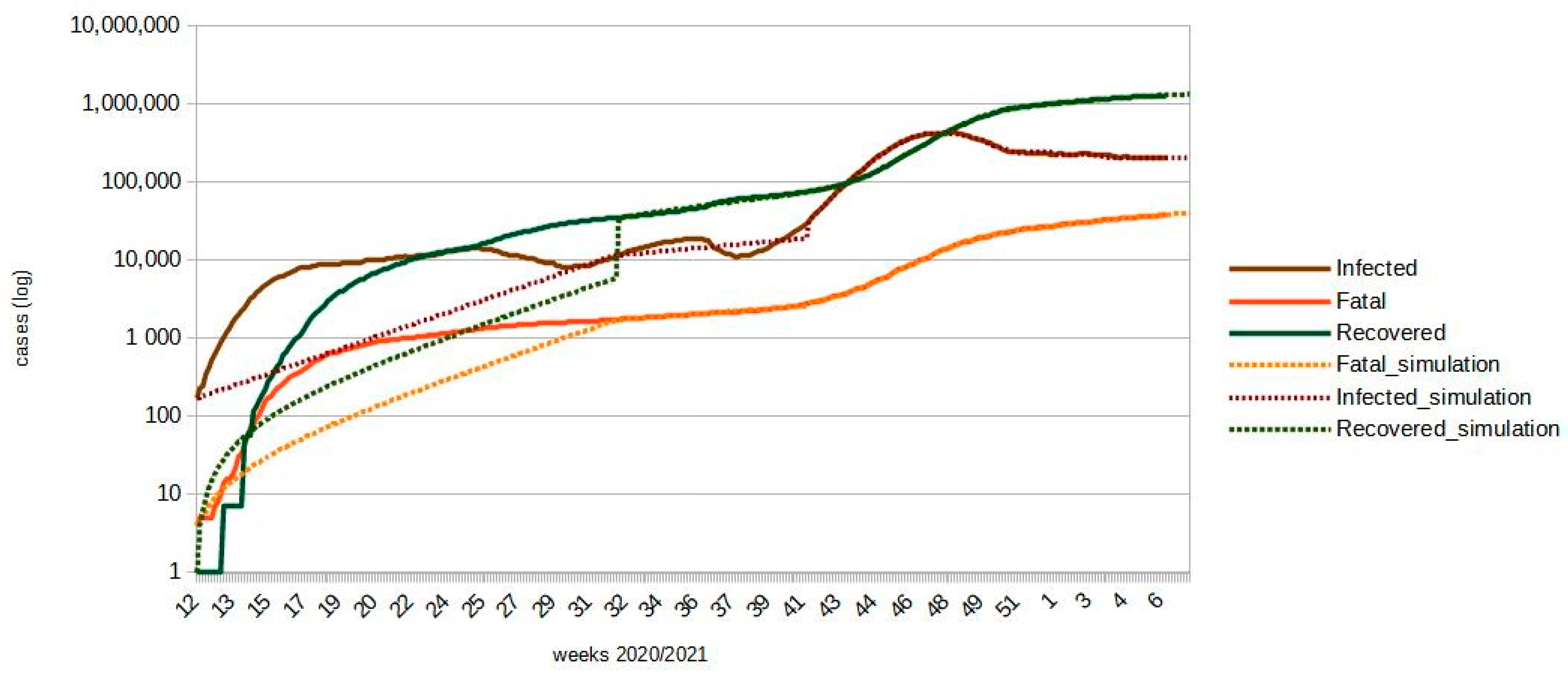
3.2. SIR-F Model Calibration

Using COVID-19 data from Poland in subsequent weeks, which were made available on government websites and in the CovsirPhy library [47,48], the values of the parameters of the SIR-F epidemiological model were estimated [49,50]. Information on the number of COVID-19 cases in Poland at the national level is presented in Figure 4.

It should be noted that data concerning the infected population involve only a fraction of the whole infected population, and only the registered fraction of the tested population is disclosed statistically. According to an officially published daily report (as of 7 February 2021), a total of 204,007 people were actually infected (1,550,255 since 4 March 2020), 1,307,161 recovered, and 39,087 failed (died, Figure 5).

Example simulation results obtained from the calibrated SIR-F model are presented in Figure 5 and Figure 6.

Figure 5 demonstrates that actual and projected values of the SIR-F model from week 40 onward are almost fitted (in logarithmic scale). In fact, there was a complete reorganization of acquisition and sharing of the COVID-19 data from the beginning of October 2020. The data before 40 weeks are burdened with uncertainty, and contain gaps.

3.3. Model Calibration–Spatial Interaction

The general spatial interaction models used in this article were calibrated by determining parameters based on the analysis of data made available by district (powiat) sanitary and epidemiological stations. The conducted analyses have shown a reliable (in a statistical sense) correlation between the number of inhabitants of individual powiats and the number of cases.

The spatial interaction models were calibrated using the generalized linear model, obtaining the logarithmic Poisson model. The authors compared the results with reference data, i.e., the number of cases in individual weeks in individual powiats in Poland. With this approach, it was possible to assess the reliability of the regression model parameters. The authors followed a similar procedure for the unconstrained gravity (Table 1, model I in

Table 2. Spatial interaction model fit statistics (* spatial verification; ** spatial prediction).

Model	Unconstrained Gravity Model (I)					Destination (Attraction) Constrained Model (III)
Week No. 2020/2021	Pseudo R2	adj. pseudo R2	AIC	SRMSE	SSI	Pseudo R2	Adj. Pseudo R2	AIC	SRMSE	SSI
15 (2020)	0.208	0. 208	557,871.6	2.69	0.25	0.74	0.74	182,944.1	1.067	0.37
20	0.197	0.197	1.72 × 106	2.14	0.31	0.82	0.82	3.89 × 105	0.74	0.47
25	0.162	0.162	4.59 × 106	4.13	0.196	0.90	0.90	5.34 × 105	1.38	0.34
28	0.162	0.162	4.795 × 106	3.50	0.22	0.899	0.899	5.75 × 105	1.22	0.38
30	0.164	0.164	3.15 × 106	3.66	0.25	0.88	0.88	4.44 × 105	1.28	0.42
33	0.235	0.235	2.55 × 106	2.57	0.32	0.86	0.86	4.80 × 105	0.99	0.51
35	0.34	0.34	3.13 × 106	2.04	0.42	0.87	0.87	6.31 × 105	0.86	0.60
36	0.44	0.44	5.17 × 106	1.63	0.44	0.89	0.89	9.72 × 105	0.81	0.63
40	0.50	0.50	3.41 × 106	2.08	0.45	0.89	0.89	7.31 × 105	1.28	0.62
48	0.78	0.78	240,549.3	23.93	0.001	0.85	0.85	167,863	19.12	0.001
49	0.77	0.77	2.25 × 105	24.69	0.001	0.845	0.844	1.55 × 105	19.79	0.002
50	0.78	0.78	205,945.5	26.42	0.001	0.849	0.848	140,473.2	20.68	0.001
51	0.77	0.77	193,757.6	27.53	0.001	0.849	0.849	130,010.9	21.87	0.001
52	0.77	0.77	91,125.6	29.32	0.001	0.851	0.849	59,741.23	22.68	0.001
1 (2021)	0.772	0.772	178,070.68	28.05	0.001	0.85	0.85	118,350.50	22.97	0.002
2	0.77	0.77	194,127.08	27.60	0.001	0.85	0.85	129,449.48	22.53	0.002
3	0.767	0.767	147,442.42	27.19	0.001	0.849	0.848	96,156.31	21.10	0.001
4	0.772	0.771	115,513.18	26.98	0.001	0.847	0.845	78,254.32	21.39	0.001
5	0.776	0.776	107,080.50	26.92	0.001	0.848	0.847	73,356.91	21.15	0.002
6 *	0.778	0.778	103,959.48	27.32	0.001	0.848	0.847	71,851.31	21.05	0.001
7 *	0.774	0.774	112,247.09	28.04	0.001	0.847	0.846	76,803.60	21.47	0.001
7 **
Charts/sparkline/for certain weeks	adj. determination coefficient		AIC	SRMSE		adj. determination coefficient		AIC	SRMSE

) and destination (Table 1, attraction model III in Table 2) models, using the population statistics as the explanatory variables for a sequence of randomly chosen weeks in 2020.

3.4. Model Verification

A verification of the destination-constrained spatial interaction models was performed for the 6th and 7th weeks of 2021 (1–7 February) using the acquired empirical aggregated data of COVID-19 infections by county. The general formula of the destination-constrained model (III) for 6th and 7th weeks of 2021 (Equations (9) and (10)):

$$T_{ij}=exp\left(-9.64087617+0.62338838 ln ln \left(V_i\right)-0.12427341-\left(-0.11015654\right) ln\left(d_{ij}\right)\right)$$

(9)

$$T_{ij}=exp\left(-9.71866096+0.63624388 ln ln \left(V_i\right)-0.12195776-\left(-0.1101434\right) ln\left(d_{ij}\right)\right)$$

(10)

where T_ij is the modeled number of infections in count j due to interaction with county i, V_i is the population of county i, and d_ij is the distance between county i and j; for the county itself, the distance taken into account was the radius of a circle of equal area to the county area.

The coefficient of determination R2 equaled 0.85, meaning that the developed model explains 85% of the variance of the phenomenon and the actual number of cases. Based on the resultant model, the authors developed a map of the residuals of regression (Figure 7a–d indicating a proportion of the number of cases not explained by the model. Table 2 provides data on the quality of the model’s fit. The determined parameter β = −0.11 shows that, in a given powiat, the average increase in the incidence will amount to 10.4%, with a population increase per unit of distance (per 1 km).

The results (Figure 7a) indicate that the developed model underestimates the actual number of infections. However, the obtained statistical data indicate the similar reliability estimates of unconstrained gravity and destination-constrained spatial interaction models.

These models fit the statistics for different time intervals, to prove that the outbreak of the COVID-19 pandemic targeted the most populated areas over time. These values are more reliable than the data concerning one-week intervals (

Table 3. Spatial interaction model fit statistics (for different time intervals in the early stages of the outbreak).

Model	Unconstrained Gravity Model					Destination (Attraction) Constrained Model
Week No. 2020	Pseudo R2	Adj. Pseudo R2	AIC	SRMSE	SSI	Pseudo R2	Adj. Pseudo R2	AIC	SRMSE	SSI
10–22/sum/	0.122	0.122	1.75 × 107	2.203	0.391	0.609	0.609	7.777 × 106	2.018	0.573
10–42/sum/	0.484	0.484	3.23 × 107	1.607	0.576	0.947	0.947	3.33 × 106	0.822	0.777
1–7 (2021)/sum/	0. 779	0. 779	925,496.67	27.18	0.001	0.851	0.851	624,561.11	21.49	0.002
1–7 (2021) sum *	0.781	0.781	915,074.37	25.19	0.001	0.864	0.864	569,191.85	18.24	0.002

* modeling using the population and commuters for counties as explanatory variables.

).

3.5. Simulation

Our model can be combined with the SIR-F model for spatial predictions. The approach is to forecast the total number of cases and then disaggregate the total number of cases to obtain the spatial distribution. This leads us to the new concept of combining the classic epidemic models with spatial interaction models proposed and developed by O’Kelly [47] and Oshan [35]. The authors used the results of the predictive simulation obtained by applying the SIR-F model to the territory of Poland to estimate the number of infections in individual powiats. Due to the unknown spatial differentiation of infections within powiats, the authors used the unconstrained gravity model for this analysis The total numbers of simulated (absolute) susceptible, infected, failed, and recovered cases in Poland from the SIR-F model are presented in

Table 4. Simulation of the SIR-F model in the sixth week of 2021.

Date	Confirmed Cases	Fatal Cases	Infected Cases	Recovered Cases	Diff. Confirmed	Diff. Fatal	Diff. Infected	Diff. Recovered
8 February 2021	1,553,164	39,478	203,234	1,310,452	6060	274	225	6011
9 February 2021	1,558,463	39,754	202,915	1,315,794	6051	274	227	6004
10 February 2021	1,563,753	40,030	202,595	1,321,128	6044	273	226	5997
11 February 2021	1,569,035	40,305	202,276	1,326,454	6036	273	228	5991
12 February 2021	1,574,307	40,580	201,956	1,331,771	6029	273	228	5984
13 February 2021	1,579,571	40,855	201,636	1,337,080	6020	272	229	5977
14 February 2021	1,603,175	41,034	203,706	1,358,435	6013	272	230	5971
Total					42,206	1909	1598	41,895

. The simulation of the SIR-F model was performed on 7 February 2021; the estimation of the unconstrained gravity model was completed at the end of the week.

The unconstrained gravity models took different forms for the first weeks (sixth and seventh weeks of 2021, Equations (11) and (12) and for the seven weeks ahead (Equation (13)). The modeling results are presented in the maps (Figure 8a–d).

$$T_{ij}=exp\left(-9.64087617+0.62260227 ln \left(V_i\right)+0.62260227 ln ln \left( W_j\right)-\left(-0.11015654\right) ln ln \left(d_{ij}\right) \right)$$

(11)

$$T_{ij}=exp\left(-9.71866096+0.62811812 ln \left(V_i\right)+0.62811812 ln ln \left( W_j\right)-\left(-0.1101434\right) ln ln \left(d_{ij}\right) \right)$$

(12)

$$T_{ij}=exp\left(-6.87909269+0.60225244 ln \left(V_i\right)+0.60225244 ln ln \left( W_j\right)-\left(-0.11531647\right) ln ln \left(d_{ij}\right) \right)$$

(13)

where T_ij is the modeled number of infections, V_i is the population of county i, W_j is the population of county j, and d_ij is the distance between counties i and j; for the county itself, the distance taken into account was the radius of a circle of area equal to the county area.

4. Discussion

The article aimed to develop a spatial interaction model using the “gravitational” approach, and test whether it adequately estimates the COVID-19 pandemic spread in Poland. The gravity model assumed the population size of individual powiats and their mutual distance as explanatory variables. The model that we developed has the advantage of combining the epidemic SIR model with the model of spatial interactions. Classical epidemic models such as SIR models provide a reliable estimate of changes over time, but do not allow for the spatial analysis of morbidity, death, or severe cases.

The results indicate that the unconstrained gravity model enables the prediction of the actual number of infections, as confirmed by the analysis carried out for the seventh week of 2021. The values obtained in the prediction are much higher than the official reports provided by district sanitary and epidemiological stations. This suggests that the actual number of cases is several times (even ten times) higher than the number of officially reported cases. The Interdisciplinary Center for Mathematical and Computational Modeling of the University of Warsaw (ICM UW) has obtained similar results [50].

Thus, the model presented in this study was calibrated in proportion to the estimated values obtained using the SIR-F model with proven reliability, while maintaining the spatial differentiation provided by the unconstrained gravity model.

Of note, the expected total number of infections in Poland was 42,206 cases (Table 4, Figure 8d) in the seventh week of 2020. The model calibrated using official data from the Ministry of Health was less reliable (Equation (13), Figure 8a,b), as it assumed that the epidemiological situation in Poland in the analyzed period was not changing rapidly.

There are at least two ways to verify the prediction of the number of infections in individual powiats. The SIR or SIR-F models were used at both the national and the district (powiat) levels, and the results were verified using a destination-constrained spatial interaction model at the district level, and an unconstrained gravity model at the national level. The promising results of this combined approach permit the hypothesis that the number of cured cases and the number of vaccinated cases should be considered additional variables in further studies. Taking these values into account would make it possible to reduce the study population susceptible to infection by the number of partially or permanently immunized. It is also possible to consider other social and demographic variables, such as age groups, employment status, and the occupational mobility of residents, among others. Including occupational mobility may be particularly crucial as it indicates the number of work-related contacts between individual administrative units. It would also be useful to consider more extended time series and to assess the credibility of the official epidemiological data provided by district sanitary and epidemiological stations to improve the prediction’s quality and credibility. One limitation of this study is that the model does not include pre-existing health problems, such as cardiovascular disease or diabetes, both of which are linked to COVID-19 infections, and in particular, to the worst outcomes. Incorporating such risk factors into COVID-19 research could be beneficial [51,52].

Moreover, the implementation of our model allows the assessment of the actual number of infections, and therefore, it can be used to predict future COVID-19 infection volumes, which provides good forecasts of an overview of future pandemic conditions [53,54]. In particular, the model can be used by central and local government administration to plan and manage efficient activities to counter the spread of COVID-19 infections. It can help with decision-making and public health resource allocation by evaluating and visualizing spatial data on infection outbreaks.

5. Conclusions

Our study has shown that spatial interaction models are an adequate tool for modeling the spatial-temporal diffusion of the COVID-19 pandemic in Poland, and for determining the number of infections. The results can also be compared with research conducted in other countries. Moreover, numerical simulations have shown that, to determine the degree of mutual influence among administrative districts in terms of pandemic spread, data on the number of inhabitants and the distances between these units are sufficient. The model developed on the basis of these assumptions explains almost 90% of the temporal and spatial variability of the phenomenon.

The data set of COVID-19 infections used included the first year of the pandemic in Poland (12 months, i.e., from March 2020 to February 2021), and there was no additional information differentiating variants of SARS-CoV-2 virus infections. The modeling was aimed only at the confirmation of the simple heuristic empirical evidence of the association between the potential (maximized, simulated) number of possible contacts and the revealed number of infections. To our knowledge, this was the first systematic approach aimed only at finding the spatial regularities of the COVID-19 pandemic in Poland. The confirmation of tested spatial trends will make it possible to introduce additional dependent (mortality or recoveries) and independent variables (e.g., mean radiative temperatures, MRT). It seems that, the shorter the period of the simulation, the greater the fit of dependent variables simulated. On the other hand, as mentioned above, some variables, such as MRT, reveal their impact during longer simulations, and there is no significance for the spatial heterogeneity of infections for short-time simulations in Poland (in fact, MRT is a confounding variable in these short periods).

Our model includes a spatial component, which allowed for the assessment of the potential spatial differentiation of the infected number of persons within a set of observed spatial units (for example, counties in Poland), which is essential in the case of COVID-19 surveillance. Hence, our model could help to assess the spatial locations of infection outbreaks, and determine the regularity of the spatial and temporal evolution of the pandemic. Therefore, the model we lay out here could be valuable to policymakers who need the geographic predictions of disease spread to make policy decisions. For example, the knowledge may provide a basis for implementing restrictions limited to specific geographic areas, based on the forecasts made with the model.

In future work, the authors aim to include the vaccination policy model as well as data on the occupational mobility of residents during the pandemic.

References

1. Werner, P. Tracing and modeling of the COVID-19 pandemic infections in Poland using spatial interactions models. In Computational Science and Its Applications—ICCSA 2021; Springer: Cham, Switzerland, 2021. [Google Scholar]
2. Rader, B.; Scarpino, S.V.; Nande, A.; Hill, A.L.; Adlam, B.; Reiner, R.C.; Pigott, D.M.; Gutierrez, B.; Zarebski, A.E.; Shrestha, M.; et al. Crowding and the shape of COVID-19 epidemics. Nat. Med. 2020, 26, 1829–1834. [Google Scholar] [CrossRef] [PubMed]
3. Petersen, E.; Koopmans, M.; Go, U.; Hamer, D.H.; Petrosillo, N.; Castelli, F.; Storgaard, M.; Al Khalili, S.; Simonsen, L. Comparing SARS-CoV-2 with SARS-CoV and influenza pandemics. Lancet Infect. Dis. 2020, 20, e238–e244. [Google Scholar] [CrossRef]
4. Huang, C.; Wang, Y.; Li, X.; Ren, L.; Zhao, J.; Hu, Y.; Zhang, L.; Fan, G.; Xu, J.; Gu, X.; et al. Clinical features of patients infected with 2019 novel coronavirus in Wuhan, China. Lancet 2020, 395, 497–506. [Google Scholar] [CrossRef] [Green Version]
5. Zhou, F.; Yu, T.; Du, R.; Fan, G.; Liu, Y.; Liu, Z.; Xiang, J.; Wang, Y.; Song, B.; Gu, X.; et al. Clinical course and risk factors for mortality of adult inpatients with COVID-19 in Wuhan, China: A retrospective cohort study. Lancet 2020, 395, 1054–1062. [Google Scholar] [CrossRef]
6. Chan, J.F.-W.; Yuan, S.; Kok, K.-H.; To, K.K.W.; Chu, H.; Yang, J.; Xing, F.; BNurs, J.L.; Yip, C.C.-Y.; Poon, R.W.-S.; et al. A familial cluster of pneumonia associated with the 2019 novel coronavirus indicating person-to-person transmission: A study of a family cluster. Lancet 2020, 395, 514–523. [Google Scholar] [CrossRef] [Green Version]
7. Grassly, N.C.; Fraser, C. Mathematical models of infectious disease transmission. Nat. Rev. Microbiol. 2008, 6, 477–487. [Google Scholar] [CrossRef] [PubMed]
8. Wilson, A.G. Entropy in Urban and Regional Modelling; Wilson, A.G., Ed.; Pion: London, UK, 1970. [Google Scholar]
9. Wilson, A. Epidemic models with geography. arXiv 2020, arXiv:2005.07673v1. Available online: https://arxiv.org/abs/2005.07673v1 (accessed on 4 December 2021).
10. Marshall, J.M.; Wu, S.L.; Sanchez, S.M.; Kiware, S.S.; Ndhlovu, M.; Ouédraogo, A.L.; Touré, M.B.; Sturrock, H.J.; Ghani, A.C.; Ferguson, N.M. Mathematical models of human mobility of relevance to malaria transmission in Africa. Sci. Rep. 2018, 8, 7713. [Google Scholar] [CrossRef] [PubMed]
11. Xia, Y.; Bjornstad, O.N.; Grenfell, B.T. Measles metapopulation dynamics: A gravity model for epidemiological coupling and dynamics. Am. Nat. 2004, 164, 267–281. [Google Scholar] [CrossRef]
12. Yan, X.-Y.; Zhou, T. Destination choice game: A spatial interaction theory on human mobility. Sci. Rep. 2019, 9, 9466. [Google Scholar] [CrossRef]
13. Stewart, J.Q. Empirical mathematical rules concerning the distribution and equilibrium of population. Geogr. Rev. 1947, 37, 461–485. [Google Scholar] [CrossRef]
14. Gregory, D.; Johnston, R.; Pratt, G.; Watts, M.; Whatmore, S. (Eds.) The Dictionary of Human Geography, 5th ed.; Wiley-Blackwell: Hoboken, NJ, USA, 2009. [Google Scholar]
15. Werner, P. Simulating of accessibility of ICT infrastructure in Poland using geographical potential models. In Proceedings of the 16th International Conference on System Science, Banff, AB, Canada, 8–12 May 2007; pp. 261–269. [Google Scholar]
16. Tobler, W.R. Cellular Geography. In Philosophy in Geography; Gale, S., Olsson, G., Eds.; Springer: Dordrecht, The Netherlands, 1979; pp. 379–386. [Google Scholar]
17. Riley, S.; Eames, K.; Isham, V.; Mollison, D.; Trapman, P. Five challenges for spatial epidemic models. Epidemics 2015, 10, 68–71. [Google Scholar] [CrossRef] [PubMed] [Green Version]
18. Rossa, F.D.; Salzano, D.; Dimeglio, A.; Bernardo, M.D.; De Lellis, M.; Coraggio, M.; Calabrese, C.; Guarino, A.; Cardona-Rivera, R.; De Lellis, P.; et al. A network model of Italy shows that intermittent regional strategies can alleviate the COVID-19 epidemic. Nat. Commun. 2020, 11, 5106. [Google Scholar] [CrossRef]
19. Parino, F.; Zino, L.; Porfiri, M.; Rizzo, A. Modeling and predicting the effect of social distancing and travel restrictions on COVID-19 spreading. JRS Interface 2021, 18, 175. [Google Scholar]
20. Gosgens, M.; Hendriks, T.; Boon, M.; Steenbakkers, W.; Heesterbeek, H.; Van der Hofstad, R.; Litvak, N. Trade-offs between mobility restrictions and transmission of SARS-CoV-2. JRS Interface 2021, 18, 175. [Google Scholar] [CrossRef]
21. Giordano, G.; Blanchini, F.; Bruno, R.; Colaneri, P.; Di Filippo, A.; Di Matteo, A.; Colaneri, M. Modelling the COVID-19 epidemic and implementation of population-wide interventions in Italy. Nat. Med. 2020, 26, 855–860. [Google Scholar] [CrossRef] [PubMed]
22. Dangermond, J.; De Vito, C.; Pesaresi, C. Using GIS in the Time of the COVID-19 Crisis, casting a glance at the future. A joint discussion. J-READING J. Res. Didat. Geogr. 2020, 1, 195–205. [Google Scholar]
23. Boulos, M.N.; Geraghty, E.M. Geographical tracking and mapping of coronavirus disease COVID-19/severe acute respiratory syndrome coronavirus 2 (SARS-CoV-2) epidemic and associated events around the world: How 21st century GIS technologies are supporting the global fight against outbreaks and epidemics. Int. J. Health Geogr. 2020, 19, 8. [Google Scholar]
24. Esaresi, C.; Pavia, D.; De Vito, C.; Barbara, A.; Cerabona, V.; Di Rosa, E. Dynamic space-time diffusion simulator in a GIS environment to tackle the Covid-19 emergency. Testing a geotechnological application in rome. Geogr. Tech. 2021, 16, 82–99. [Google Scholar]
25. Franch-Pardo, I.; Napoletano, B.M.; Rosete-Verges, F.; Billa, L. Spatial analysis and GIS in the study of COVID-19. A review. Sci. Total Environ. 2020, 739, 140033. [Google Scholar] [CrossRef] [PubMed]
26. Hohl, A.; Delmelle, E.M.; Desjardins, M.R.; Lan, Y. Daily surveillance of COVID-19 using the prospective space-time scan statistic in the United States. Spat. Spatio-Temporal Epidemiol. 2020, 34, 100354. [Google Scholar] [CrossRef] [PubMed]
27. Ahasan, R.; Hossain, M.M. Leveraging GIS and spatial analysis for informed decision-making in COVID-19 pandemic. Health Policy Technol. 2021, 10, 7. [Google Scholar] [CrossRef] [PubMed]
28. Wu, Z.; McGoogan, J.M. Characteristics of and Important Lessons from the Coronavirus Disease 2019 (COVID-19) Outbreak in China: Summary of a Report of 72 314 Cases from the Chinese Center for Disease Control and Prevention. JAMA 2020, 323, 1239–1242. [Google Scholar] [CrossRef] [PubMed]
29. Zhang, X.; Rao, H.; Wu, Y.; Huang, Y.; Dai, H. Comparison of spatiotemporal characteristics of the COVID-19 and SARS outbreaks in mainland China. BMC Infect Dis. 2020, 20, 805. [Google Scholar] [CrossRef] [PubMed]
30. Brauer, F.; Castillo-Chavez, C. Mathematical Models in Population Biology and Epidemiology; Texts in Applied Mathematics; Springer: New York, NY, USA, 2012; Volume 40, ISBN 978-1-4614-1685-2. [Google Scholar]
31. Duan, W.; Fan, Z.; Zhang, P.; Guo, G.; Qiu, X. Mathematical and Computational Approaches to Epidemic Modeling: A Comprehensive Review. Front. Comput. Sci. 2015, 9, 806–826. [Google Scholar] [CrossRef] [PubMed]
32. Casetti, E. Expansion Method, Dependency, and Multimodeling. In Handbook of Applied Spatial Analysis; Fischer, M.M., Getis, A., Eds.; Springer: Berlin/Heidelberg, Germany, 2010; pp. 487–505. ISBN 978-3-642-03646-0. [Google Scholar]
33. Kermack, W.O.; McKendric, A.G. A contribution to the mathematical theory of epidemics. Proc. R. Soc. Lond. Ser. A Contain. Pap. A Math. Phys. Character 1927, 115, 700–721. [Google Scholar] [CrossRef] [Green Version]
34. Abadie, A.; Bertolotti, P.; Deaner, B.; Shah, D. Epidemic Modeling and Estimation. 2020. Available online: https://idss.mit.edu/wp-content/uploads/2020/04/04.28.2020Epidemic_Modeling_A_Memo.pdf (accessed on 4 December 2021).
35. Oshan, T.M. A primer for working with the Spatial Interaction modeling (SpInt) module in the python spatial analysis library (PySAL). Region 2016, 3, R11–R23. [Google Scholar] [CrossRef]
36. McFadden, D. Conditional logit analysis of qualitative choice behaviour. In Frontiers in Econometrics; Zarembka, P., Ed.; Academic Press: New York, NY, USA, 1974; pp. 105–142. [Google Scholar]
37. Akaike, H. A new look at the statistical model identification. IEEE Trans. Autom. Control 1974, 19, 716–723. [Google Scholar] [CrossRef]
38. Rey, S.J.; Anselin, L. PySAL: A Python library of spatial analytical methods. Rev. Reg. Stud. 2007, 37, 5–27. [Google Scholar] [CrossRef]
39. Raport Zakażeń Koronawirusem (SARS-CoV-2). 2021. Available online: https://www.gov.pl/web/koronawirus/wykaz-zarazen-koronawirusem-sars-cov-2 (accessed on 6 December 2021).
40. Morrill, R.; Gaile, G.; Thrall, G. Spatial Diffusion. In Web Book of Regional Science; West Virginia University: Morgantown, WV, USA, 2020. [Google Scholar]
41. Wilson, A.G. Complex Spatial Systems: The Modelling Foundations of Urban and Regional Analysis; Pearson Education: London, UK, 2000. [Google Scholar]
42. O’Kelly, M.E. Spatial Interaction Models. In International Encyclopedia of Human Geography; Kitchin, R., Thrift, N., Eds.; Elsevier: Amsterdam, The Netherlands, 2009; pp. 365–368. [Google Scholar]
43. Coronavirus: Information and recommendations. Temporary Limitations. 2021. Available online: https://www.gov.pl/web/coronavirus/temporary-limitations (accessed on 6 December 2021).
44. Government Data Shared on Twitter. Available online: https://twitter.com/MZ_GOV_PL (accessed on 8 December 2021).
45. Główny Urząd Geodezji i Kartografii. 2021. Available online: http://www.gugik.gov.pl/pzgik/inne-dane-udostepniane-bezplatnie (accessed on 4 December 2021).
46. Bank Danych Lokalnych GUS. 2021. Available online: https://bdl.stat.gov.pl/BDL/start (accessed on 4 December 2021).
47. CovsirPhy Development Team. CovsirPhy, Python Package for COVID-19 Analysis with SIR-Derived ODE Models. 2020. Available online: https://github.com/lisphilar/covid19-sir (accessed on 4 December 2021).
48. Guidotti, E.; Ardia, D. COVID-19 Data Hub. J. Open Source Softw. 2020, 5, 2376. [Google Scholar] [CrossRef]
49. Fotheringham, A.S.; O’Kelly, M.E. Spatial Interaction Models: Formulations and Applications; Kluwer Academic Publishers: Alphen aan Den Rijn, The Netherlands, 1989. [Google Scholar]
50. ICM UW Model Description—COVID. Available online: https://covid-19.icm.edu.pl/ (accessed on 4 December 2021).
51. Zhu, D.; Ye, X.; Manson, S. Revealing the spatial shifting pattern of COVID-19 pandemic in the United States. Sci. Rep. 2021, 11, 8396. [Google Scholar] [CrossRef] [PubMed]
52. Mhango, M.; Dzobo, M.; Chitungo, I.; Dzinamarira, T. COVID-19 risk factors among health workers: A rapid review. Saf. Health Work 2020, 11, 262–265. [Google Scholar] [CrossRef] [PubMed]
53. Tahmasebi, P.; Shokri-Kuehni, S.M.; Sahimi, M.; Shokri, N. How do environmental, economic and health factors influence regional vulnerability to COVID-19? MedRxiv 2020. Available online: https://www.medrxiv.org/content/10.1101/2020.04.09.20059659v1 (accessed on 23 November 2021).
54. Werner, P.A.; Skrynyk, O.; Porczek, M.; Szczepankowska-Bednarek, U.; Olszewski, R.; Kęsik-Brodacka, M. The Effects of Climate and Bioclimate on COVID-19 Cases in Poland. Remote Sens. 2021, 13, 4946. [Google Scholar] [CrossRef]
Figure 1. Stacked, cumulative number of infections by county in Poland per week (from March 2020 to July 2021; Study Period from weeks 11 to 41 of 2020); data source: Ministry of Health, Poland (counties are identified by statistical numbers, four-digit TERYT strings).
Ijgi 11 00195 g001
Figure 2. Total number of infections by county in Poland (from weeks 11 to 42 of 2020); our study was based on data from the Ministry of Health, Poland.
Ijgi 11 00195 g002
Figure 3. Total number of infections by county in Poland (from weeks 48 to 52 of 2020); our study was based on data from the Ministry of Health, Poland.
Ijgi 11 00195 g003
Figure 4. Poland, COVID-19: Cases over time with monotonically increasing complemented recovered data (as of 7 February 2021; results: CovsirPhy Python Application).
Ijgi 11 00195 g004
Figure 5. Poland, COVID-19: Simulation of cases over time (as of 13 February 2021; results: CovsirPhy Python Application).
Ijgi 11 00195 g005
Figure 6. Poland COVID-19: reproduction number over time (as of 13 February 2021; results: CovsirPhy Python Application).
Ijgi 11 00195 g006
Figure 7. Destination-constrained model: COVID-19 infections in Poland by county; sixth week of 2021—map of the modeled values (a) and residuals ((b), modeled—real value); seventh week of 2021—map of modeled values (c) and residuals (d).
Ijgi 11 00195 g007aIjgi 11 00195 g007bIjgi 11 00195 g007cIjgi 11 00195 g007d
Figure 8. Simulation of COVID-19-infected cases in Poland; (a) model of infected cases—seven weeks of 2021; aggregated unconstrained gravity model; (b) Residuals of infected cases—seven weeks of 2021; aggregated unconstrained gravity model; (c) Simulation of infected cases based on seven weeks of 2021; aggregated unconstrained gravity model calibrated using SIR-F models; (d) Simulation of infected cases—seventh week of 2021; aggregated unconstrained gravity model calibrated using SIR-F models.
Ijgi 11 00195 g008