
Point Event Cluster Detection via the Bayesian Generalized Fused Lasso


Abstract
:1. Introduction
2. Sparse-Modeling-Based Cluster Detection
2.1. Fused Lasso and Generalized Fused Lasso
2.2. Sparse-Modeling-Based Cluster Detection
3. Previous Studies on Sparsity-Inducing Priors
3.1. Bayesian Lasso
3.2. Bayesian Generalized Fused Lasso
4. Proposed Method
4.1. Likelihood and Prior Distributions
4.2. Tuning Hyperparameters with the Watanabe–Akaike Information Criterion
5. Evaluation
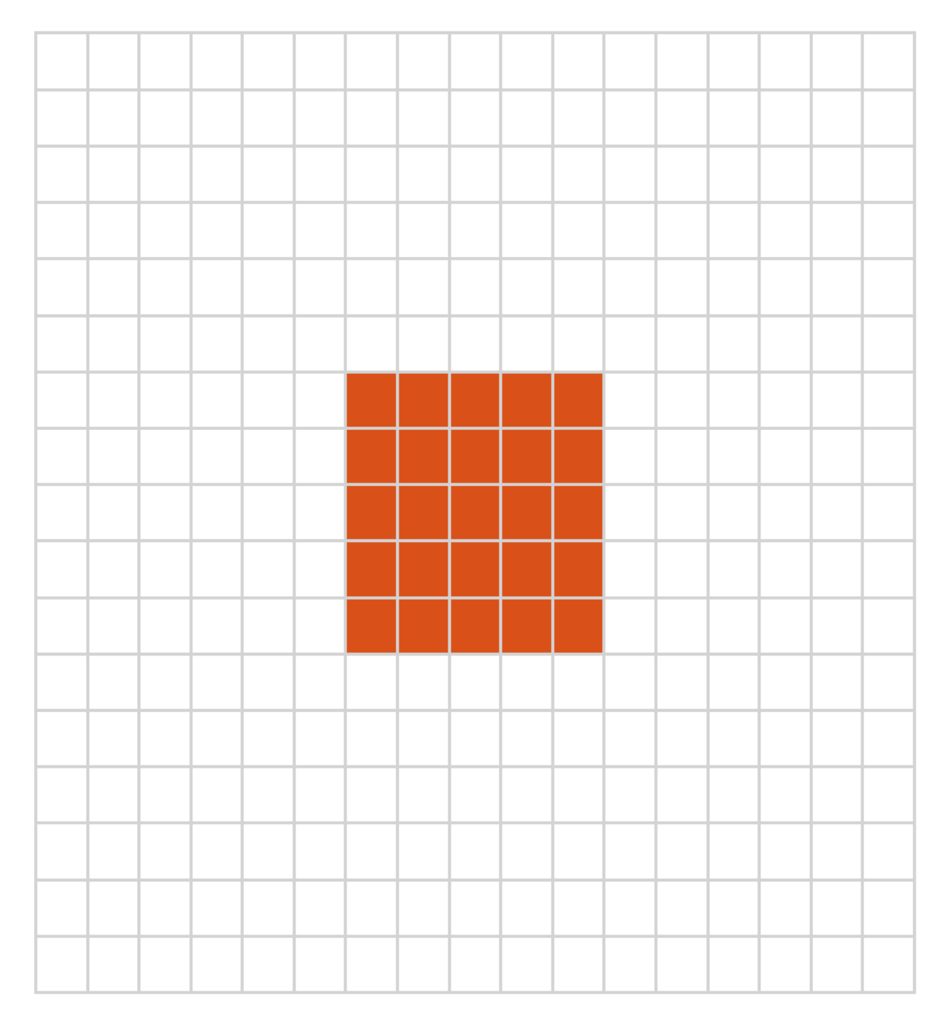
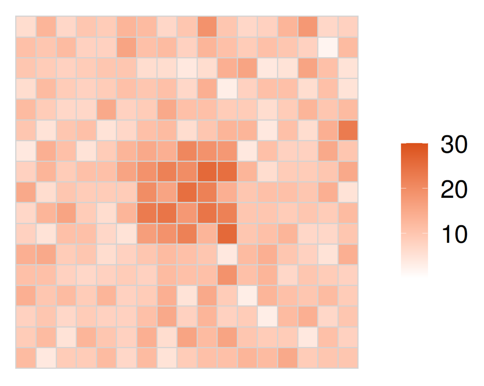
5.1. Evaluations with Simulated Distributions
5.1.1. Overview
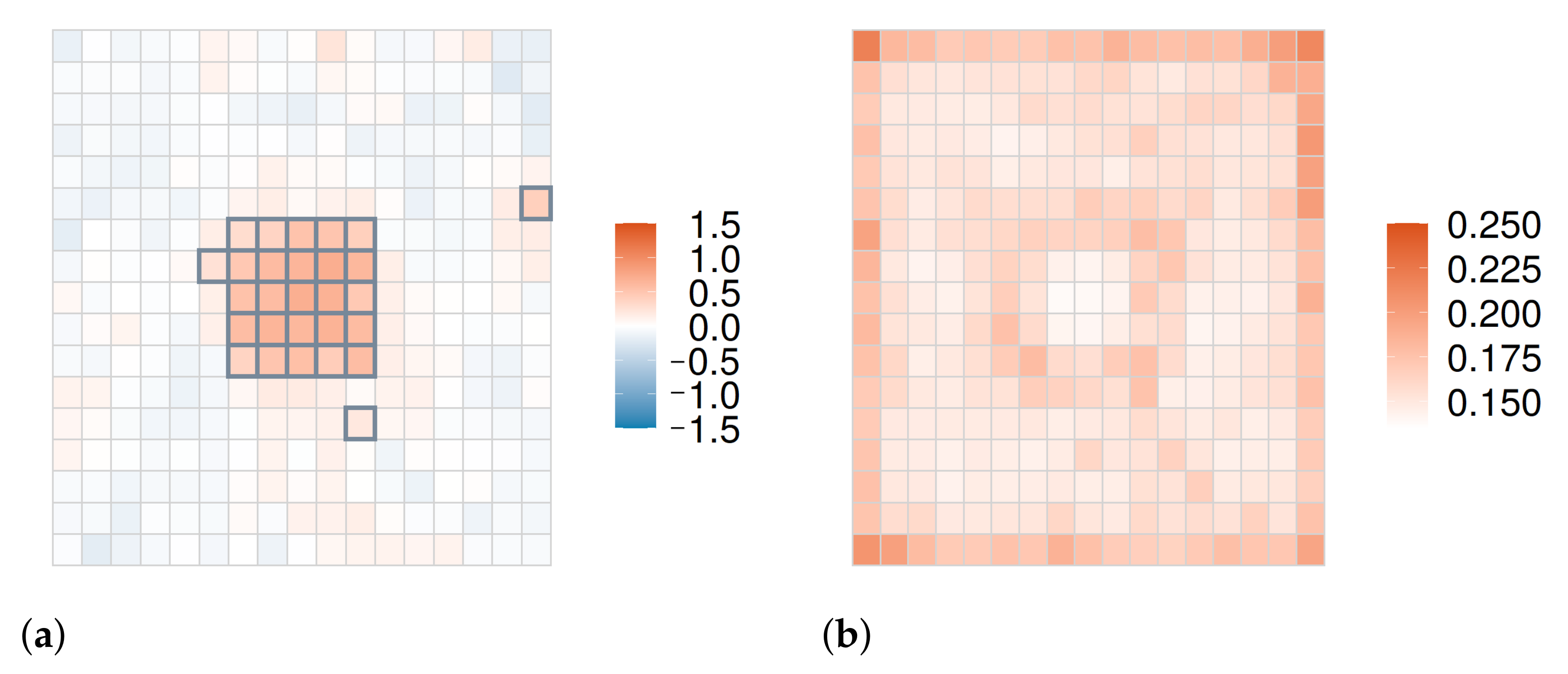
5.1.2. Results
5.2. Evaluations with Real-World Data
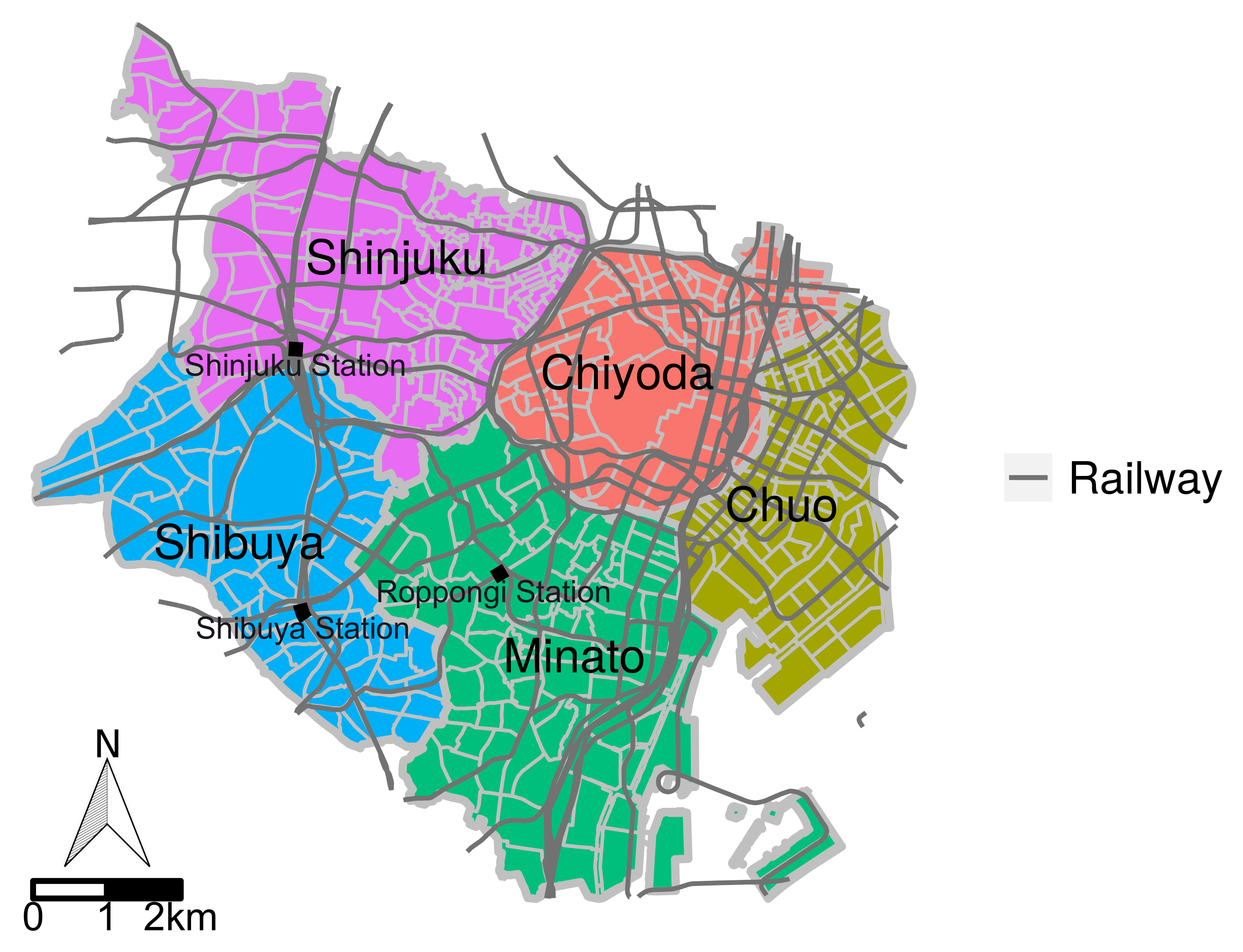
5.2.1. Target Area and Data Description
5.2.2. Estimation Settings
5.2.3. Results
5.3. Discussion
6. Conclusions
Author Contributions
Funding
Data Availability Statement
Conflicts of Interest
References
- Getis, A.; Ord, J.K. The analysis of spatial association by use of distance statistics. Geogr. Anal. 1992, 24, 189–206. [Google Scholar] [CrossRef]
- Anselin, L. Local indicators of spatial association—LISA. Geogr. Anal. 1995, 27, 93–115. [Google Scholar] [CrossRef]
- Kulldorff, M.; Nagarwalla, N. Spatial disease clusters: Detection and inference. Stat. Med. 1995, 14, 799–810. [Google Scholar] [CrossRef] [PubMed]
- Kulldorff, M. SaTScan v10.0.2: Software for the Spatial, Temporal, and Space-Time Scan Statistics. 2022. Available online: https://www.satscan.org/ (accessed on 25 February 2022).
- Huang, L.; Kulldorff, M.; Gregorio, D. A spatial scan statistic for survival data. Biometrics 2007, 63, 109–118. [Google Scholar] [CrossRef] [PubMed] [Green Version]
- Jung, I. Spatial scan statistics for matched case–control data. PLoS ONE 2019, 14, e0221225. [Google Scholar] [CrossRef]
- Takahashi, K.; Shimadzu, H. Detecting multiple spatial disease clusters: Information criterion and scan statistic approach. Int. J. Health Geogr. 2020, 19, 1–11. [Google Scholar] [CrossRef]
- Duczmal, L.; Assuncao, R. A simulated annealing strategy for the detection of arbitrarily shaped spatial clusters. Comput. Stat. Data Anal. 2004, 45, 269–286. [Google Scholar] [CrossRef]
- Duczmal, L.; Cançado, A.L.; Takahashi, R.H.; Bessegato, L.F. A genetic algorithm for irregularly shaped spatial scan statistics. Comput. Stat. Data Anal. 2007, 52, 43–52. [Google Scholar] [CrossRef]
- Caldas de Castro, M.; Singer, B.H. Controlling the false discovery rate: A new application to account for multiple and dependent tests in local statistics of spatial association. Geogr. Anal. 2006, 38, 180–208. [Google Scholar] [CrossRef]
- Brunsdon, C.; Charlton, M. An assessment of the effectiveness of multiple hypothesis testing for geographical anomaly detection. Environ. Plan. Plan. Des. 2011, 38, 216–230. [Google Scholar] [CrossRef]
- Choi, H.; Song, E.; Hwang, S.S.; Lee, W. A modified generalized lasso algorithm to detect local spatial clusters for count data. AStA Adv. Stat. Anal. 2018, 102, 537–563. [Google Scholar] [CrossRef]
- Tibshirani, R.J.; Taylor, J. The solution path of the generalized lasso. Ann. Stat. 2011, 39, 1335–1371. [Google Scholar] [CrossRef] [Green Version]
- Hunter, D.R.; Li, R. Variable selection using MM algorithms. Ann. Stat. 2005, 33, 1617–1642. [Google Scholar] [CrossRef] [PubMed] [Green Version]
- Tibshirani, R.J. Regression shrinkage and selection via the lasso. J. R. Stat. Soc. Ser. B (Methodol.) 1996, 58, 267–288. [Google Scholar] [CrossRef]
- Park, T.; Casella, G. The Bayesian lasso. J. Am. Stat. Assoc. 2008, 103, 681–686. [Google Scholar] [CrossRef]
- Kyung, M.; Gill, J.; Ghosh, M.; Casella, G. Penalized regression, standard errors, and Bayesian lassos. Bayesian Anal. 2010, 5, 369–411. [Google Scholar]
- Tibshirani, R.; Saunders, M.; Rosset, S.; Zhu, J.; Knight, K. Sparsity and smoothness via the fused lasso. J. R. Stat. Soc. Ser. B (Stat. Methodol.) 2005, 67, 91–108. [Google Scholar] [CrossRef] [Green Version]
- Inoue, R.; Ishiyama, R.; Sugiura, A. Identification of geographical segmentation of the rental housing market in the Tokyo metropolitan area by generalized fused lasso. J. Jpn. Soc. Civ. Eng. Ser. D3 (Infrastruct. Plan. Manag.) 2020, 76, 251–263. (In Japanese) [Google Scholar] [CrossRef]
- Inoue, R.; Ishiyama, R.; Sugiura, A. Identifying local differences with fused-MCP: An apartment rental market case study on geographical segmentation detection. Jpn. J. Stat. Data Sci. 2020, 3, 183–214. [Google Scholar] [CrossRef] [Green Version]
- Akaike, H. A new look at the statistical model identification. IEEE Trans. Autom. Control. 1974, 19, 716–723. [Google Scholar] [CrossRef]
- Schwarz, G. Estimating the dimension of a model. Ann. Stat. 1978, 6, 461–464. [Google Scholar] [CrossRef]
- Watanabe, S. Asymptotic equivalence of Bayes cross validation and widely applicable information criterion in singular learning theory. J. Mach. Learn. Res. 2010, 11, 3571–3594. [Google Scholar]
- Gelman, A.; Hwang, J.; Vehtari, A. Understanding predictive information criteria for Bayesian models. Stat. Comput. 2014, 24, 997–1016. [Google Scholar] [CrossRef]
- Duane, S.; Kennedy, A.D.; Pendleton, B.J.; Roweth, D. Hybrid monte carlo. Phys. Lett. B 1987, 195, 216–222. [Google Scholar] [CrossRef]
- Gelman, A.; Rubin, D.B. Inference from iterative simulation using multiple sequences. Stat. Sci. 1992, 7, 457–472. [Google Scholar] [CrossRef]
- Shiode, S. Street-level spatial scan statistic and STAC for analysing street crime concentrations. Trans. GIS 2011, 15, 365–383. [Google Scholar] [CrossRef]
- Fan, J.; Li, R. Variable selection via nonconcave penalized likelihood and its oracle properties. J. Am. Stat. Assoc. 2001, 96, 1348–1360. [Google Scholar] [CrossRef]
- Griffin, J.E.; Brown, P.J. Bayesian hyper-lassos with non-convex penalization. Aust. N. Z. J. Stat. 2011, 53, 423–442. [Google Scholar] [CrossRef]
- Carvalho, C.M.; Polson, N.G.; Scott, J.G. Handling sparsity via the horseshoe. J. Mach. Learn. Res. 2009, 5, 73–80. [Google Scholar]
- Carvalho, C.M.; Polson, N.G.; Scott, J.G. The horseshoe estimator for sparse signals. Biometrika 2010, 97, 465–480. [Google Scholar] [CrossRef] [Green Version]

| Hyperparameters (Equation (13)) | Candidate Values |
|---|---|
| (Unnecessary because this evaluation introduces no covariates.) |
| Hyperparameters (Equation (7)) | Candidate Values |
|---|---|
| (Unnecessary because this evaluation introduces no covariates.) |
| Method | Expected Points Outside a Cluster | Point Density Ratio | ||||
|---|---|---|---|---|---|---|
| 1.25 | 1.5 | 2.0 | 2.5 | 3.0 | ||
| Choi’s method | 10 | 0.035 | 0.733 | 0.997 | 1.000 | 1.000 |
| 20 | 0.096 | 0.927 | 0.999 | 1.000 | 1.000 | |
| 30 | 0.153 | 0.994 | 1.000 | 1.000 | 1.000 | |
| Proposed method | 10 | 0.071 | 0.599 | 0.964 | 0.998 | 1.000 |
| 20 | 0.258 | 0.882 | 0.998 | 1.000 | 1.000 | |
| 30 | 0.470 | 0.942 | 1.000 | 1.000 | 1.000 | |
| Method | Expected Points Outside a Cluster | Point Density Ratio | ||||
|---|---|---|---|---|---|---|
| 1.25 | 1.5 | 2.0 | 2.5 | 3.0 | ||
| Choi’s method | 10 | 0.003 | 0.018 | 0.020 | 0.026 | 0.013 |
| 20 | 0.003 | 0.011 | 0.006 | 0.003 | 0.001 | |
| 30 | 0.006 | 0.009 | 0.008 | 0.008 | 0.012 | |
| Proposed method | 10 | 0.005 | 0.009 | 0.018 | 0.020 | 0.017 |
| 20 | 0.006 | 0.012 | 0.015 | 0.014 | 0.014 | |
| 30 | 0.009 | 0.018 | 0.018 | 0.017 | 0.019 | |
| Hyperparameters (in Equation (13)) | Candidate Values |
|---|---|
Publisher’s Note: MDPI stays neutral with regard to jurisdictional claims in published maps and institutional affiliations. |
© 2022 by the authors. Licensee MDPI, Basel, Switzerland. This article is an open access article distributed under the terms and conditions of the Creative Commons Attribution (CC BY) license (https://creativecommons.org/licenses/by/4.0/).
Share and Cite
Masuda, R.; Inoue, R. Point Event Cluster Detection via the Bayesian Generalized Fused Lasso. ISPRS Int. J. Geo-Inf. 2022, 11, 187. https://doi.org/10.3390/ijgi11030187
Masuda R, Inoue R. Point Event Cluster Detection via the Bayesian Generalized Fused Lasso. ISPRS International Journal of Geo-Information. 2022; 11(3):187. https://doi.org/10.3390/ijgi11030187
Chicago/Turabian StyleMasuda, Ryo, and Ryo Inoue. 2022. "Point Event Cluster Detection via the Bayesian Generalized Fused Lasso" ISPRS International Journal of Geo-Information 11, no. 3: 187. https://doi.org/10.3390/ijgi11030187
APA StyleMasuda, R., & Inoue, R. (2022). Point Event Cluster Detection via the Bayesian Generalized Fused Lasso. ISPRS International Journal of Geo-Information, 11(3), 187. https://doi.org/10.3390/ijgi11030187