
Multi-Resolution Transformer Network for Building and Road Segmentation of Remote Sensing Image


Abstract
:1. Introduction
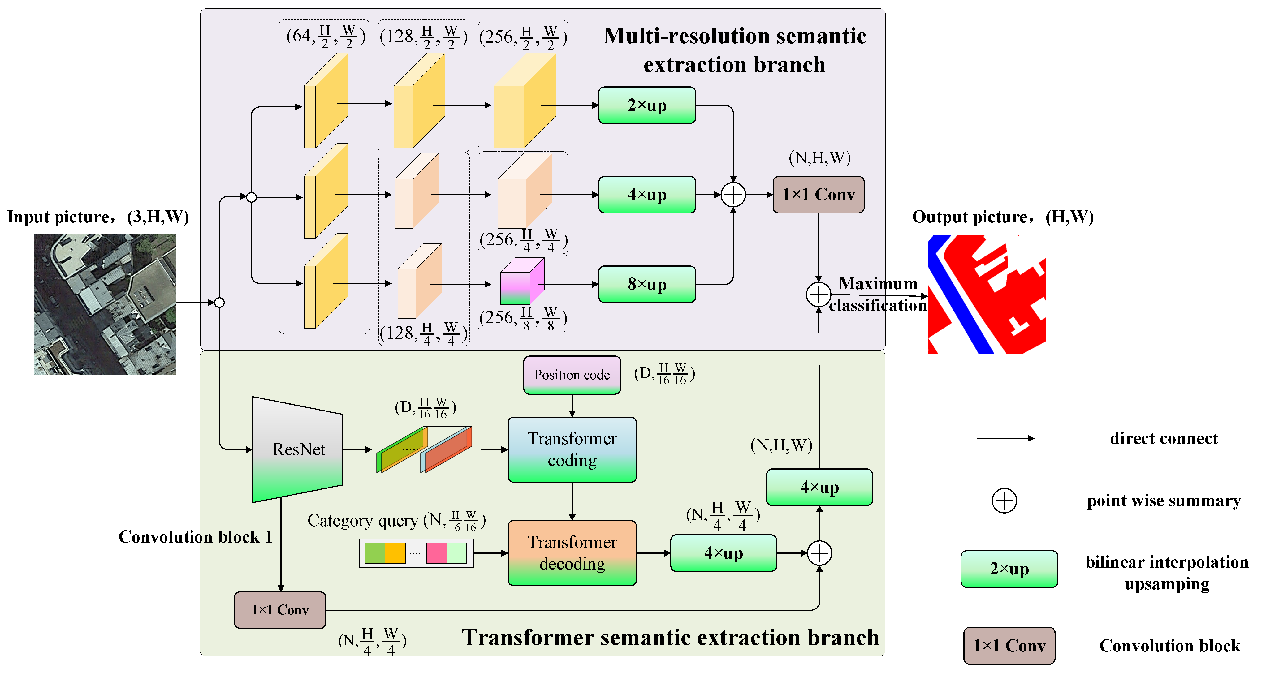
2. Methodology
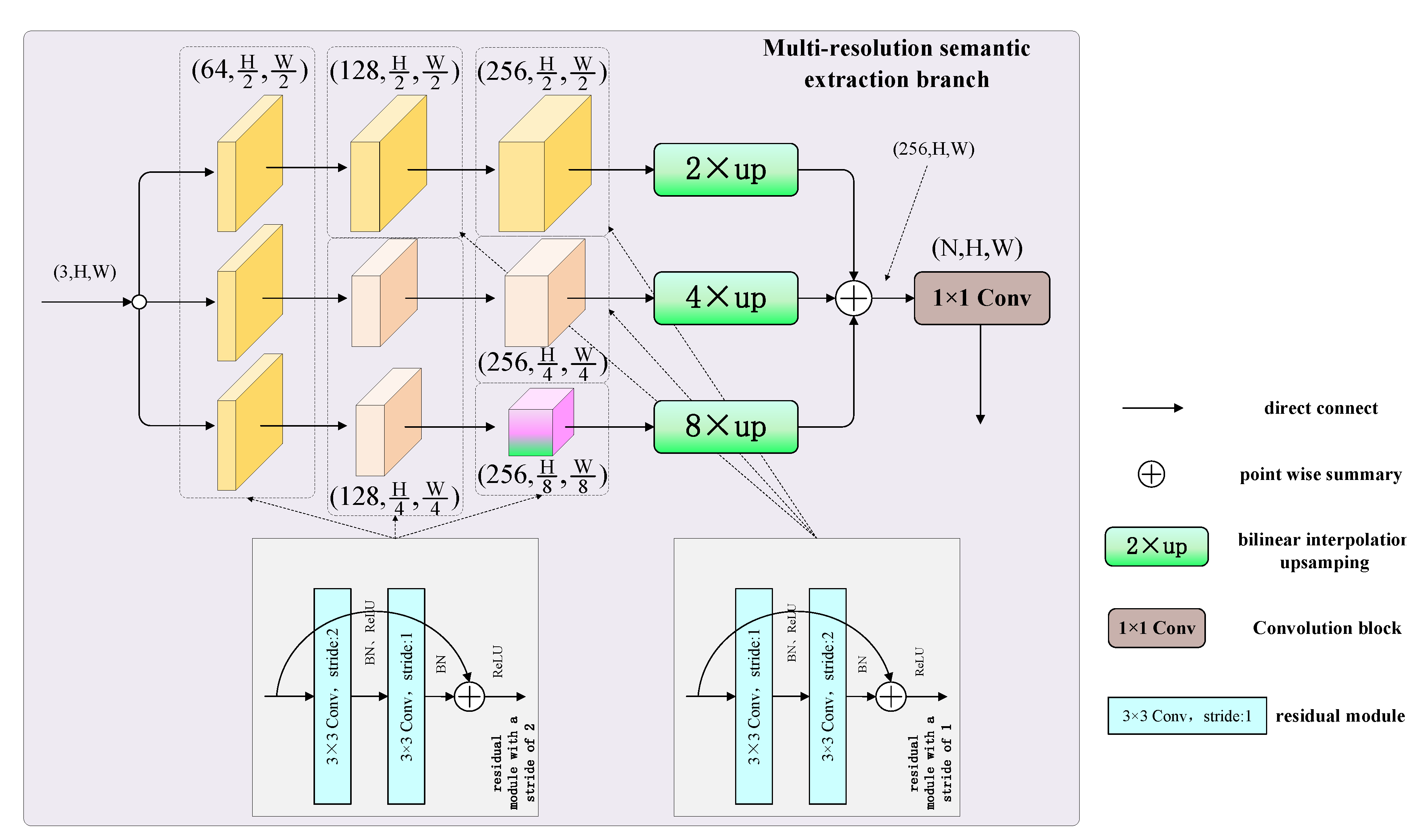
2.1. Multi-Resolution Semantic Extraction Branch
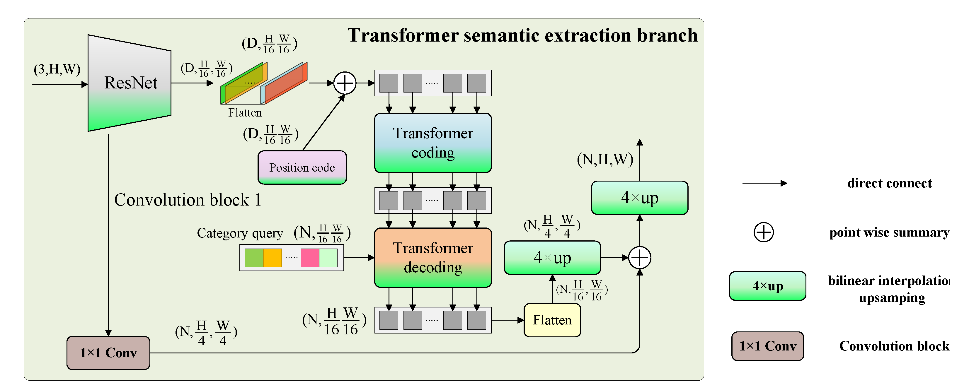
2.2. Transformer Semantic Extraction Branch
2.2.1. The Overall Framework of Transformer Semantic Extraction Branch
2.2.2. The Feature Extraction of Backbone Network
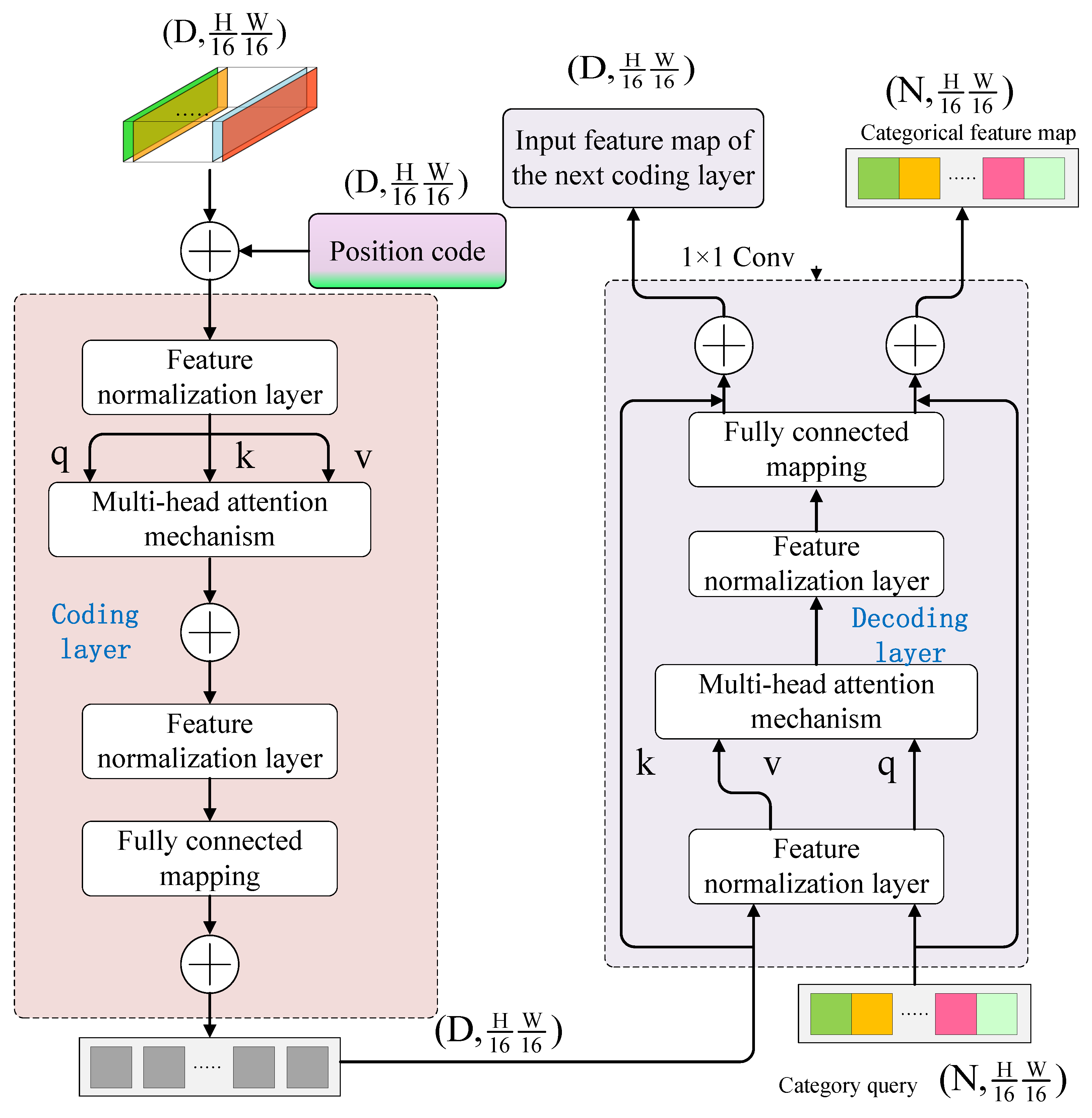
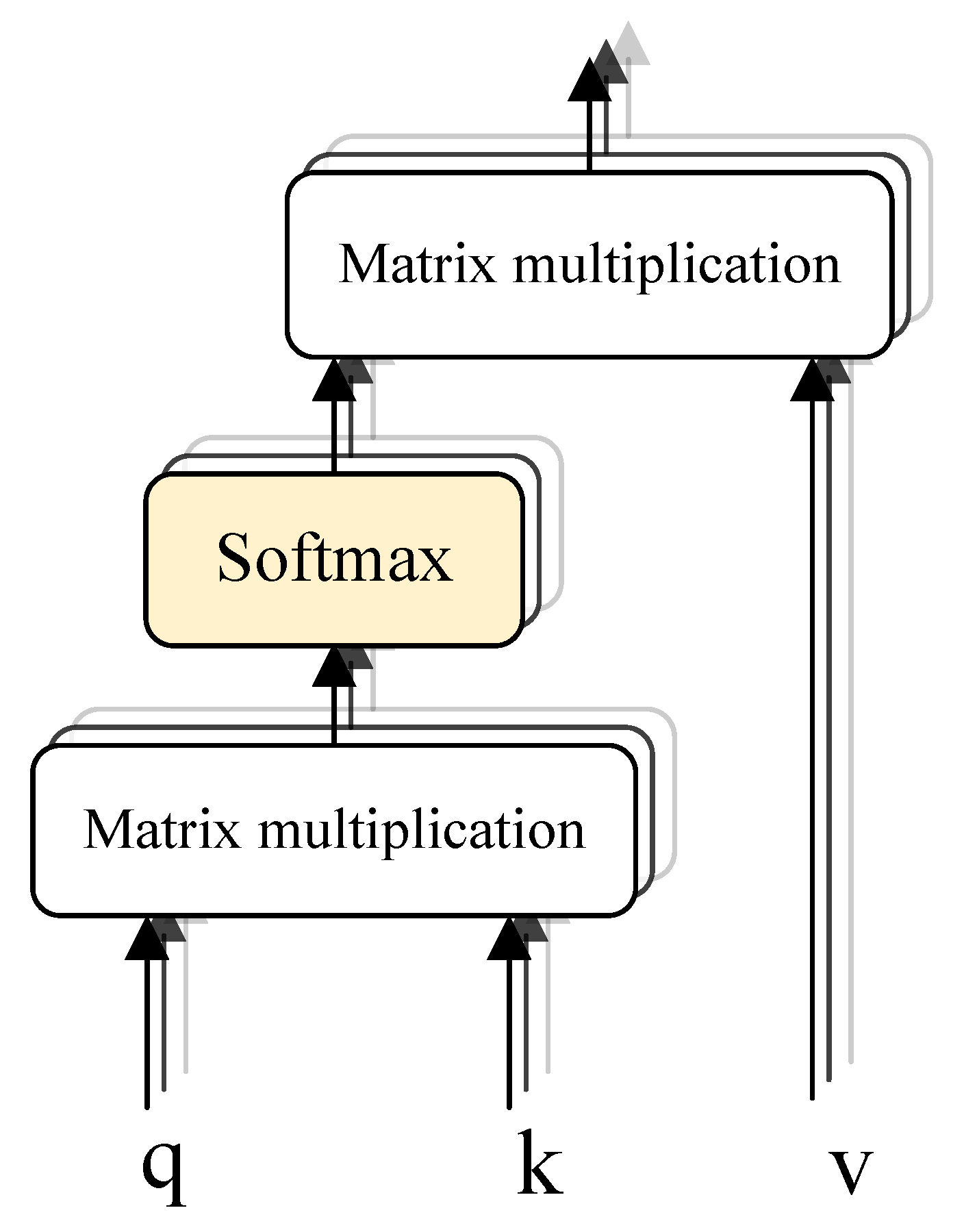
2.2.3. Transformer Encoding and Decoding
3. Experiment and Result Analysis
3.1. Datasets
3.1.1. AISD Dataset
3.1.2. ISPRS Dataset
3.2. Implementation Details
3.3. Analysis of Results
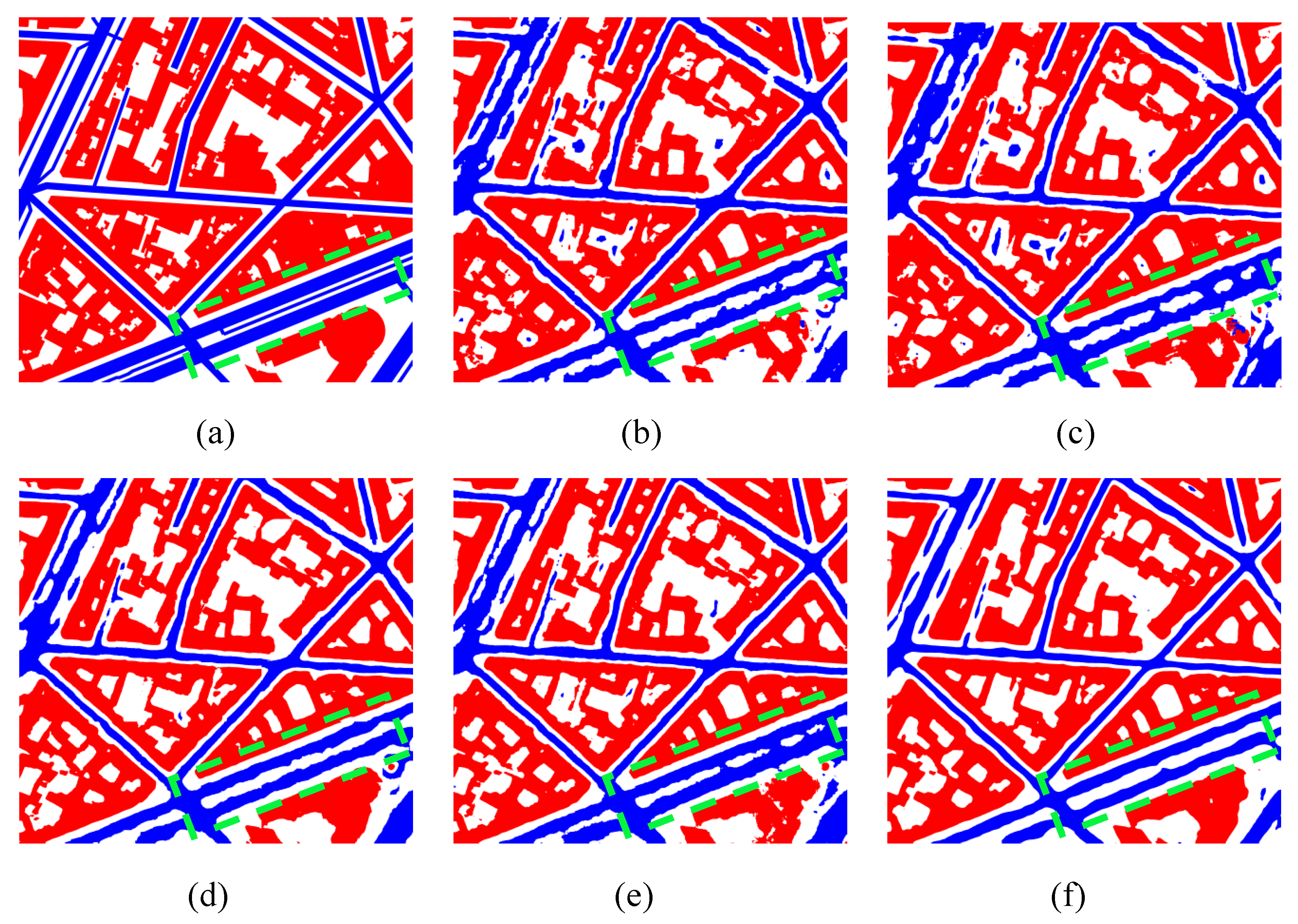
3.3.1. Evaluation Metrics and Prediction Effect
- (1)
- Main experiment
- (2)
- Generalization experimental
3.3.2. Quantitative Analysis of Model Prediction Results Promotion Strategy
4. Conclusions
Author Contributions
Funding
Institutional Review Board Statement
Informed Consent Statement
Data Availability Statement
Conflicts of Interest
References
- Pham, H.M.; Yamaguchi, Y.; Bui, T.Q. A case study on the relation between city planning and urban growth using remote sensing and spatial metrics. Landsc. Urban Plan. 2011, 100, 223–230. [Google Scholar] [CrossRef]
- Song, L.; Xia, M.; Jin, J.; Qian, M.; Zhang, Y. SUACDNet: Attentional change detection network based on siamese U-shaped structure. Int. J. Appl. Earth Obs. Geoinf. 2021, 105, 102597. [Google Scholar] [CrossRef]
- Xia, M.; Qu, Y.; Lin, H. PADANet: Parallel asymmetric double attention network for clouds and its shadow detection. J. Appl. Remote Sens. 2021, 15, 046512. [Google Scholar] [CrossRef]
- Wen, Q.; Jiang, K.; Wang, W.; Liu, Q.; Guo, Q.; Li, L.; Wang, P. Automatic building extraction from google earth images under complex backgrounds based on deep instance segmentation network. Sensors 2019, 19, 333. [Google Scholar] [CrossRef] [PubMed] [Green Version]
- Behera, M.D.; Gupta, A.K.; Barik, S.K.; Das, P.; Panda, R.M. Use of satellite remote sensing as a monitoring tool for land and water resources development activities in an Indian tropical site. Environ. Monit. Assess. 2018, 190, 401. [Google Scholar] [CrossRef]
- Qu, Y.; Xia, M.; Zhang, Y. Strip pooling channel spatial attention network for the segmentation of cloud and cloud shadow. Comput. Geosci. 2021, 157, 104940. [Google Scholar] [CrossRef]
- Yuan, J.; Wang, D.; Li, R. Remote sensing image segmentation by combining spectral and texture features. IEEE Trans. Geosci. Remote Sens. 2013, 52, 16–24. [Google Scholar] [CrossRef]
- Li, D.; Zhang, G.; Wu, Z.; Yi, L. An edge embedded marker-based watershed algorithm for high spatial resolution remote sensing image segmentation. IEEE Trans. Image Process. 2010, 19, 2781–2787. [Google Scholar] [PubMed]
- Fan, J.; Han, M.; Wang, J. Single point iterative weighted fuzzy C-means clustering algorithm for remote sensing image segmentation. Pattern Recognit. 2009, 42, 2527–2540. [Google Scholar] [CrossRef]
- Panboonyuen, T.; Vateekul, P.; Jitkajornwanich, K.; Lawawirojwong, S. An enhanced deep convolutional encoder-decoder network for road segmentation on aerial imagery. In Proceedings of the International Conference on Computing and Information Technology 2017, Helsinki, Finland, 21–23 August 2017; pp. 191–201. [Google Scholar] [CrossRef]
- Clevert, D.A.; Unterthiner, T.; Hochreiter, S. Fast and accurate deep network learning by exponential linear units (elus). arXiv 2015, arXiv:1511.07289. [Google Scholar]
- Badrinarayanan, V.; Kendall, A.; Cipolla, R. Segnet: A deep convolutional encoder-decoder architecture for image segmentation. IEEE Trans. Pattern Anal. Mach. Intell. 2017, 39, 2481–2495. [Google Scholar] [CrossRef] [PubMed]
- Sun, W.; Wang, R. Fully convolutional networks for semantic segmentation of very high resolution remotely sensed images combined with DSM. IEEE Geosci. Remote Sens. Lett. 2018, 15, 474–478. [Google Scholar] [CrossRef]
- Liu, W.; Zhang, Y.; Fan, H.; Zou, Y.; Cui, Z. A New Multi-Channel Deep Convolutional Neural Network for Semantic Segmentation of Remote Sensing Image. IEEE Access 2020, 8, 131814–131825. [Google Scholar] [CrossRef]
- Qi, X.; Li, K.; Liu, P.; Zhou, X.; Sun, M. Deep Attention and Multi-Scale Networks for Accurate Remote Sensing Image Segmentation. IEEE Access 2020, 8, 146627–146639. [Google Scholar] [CrossRef]
- Li, J.; Xiu, J.; Yang, Z.; Liu, C. Dual Path Attention Net for Remote Sensing Semantic Image Segmentation. ISPRS Int. J. Geo-Inf. 2020, 9, 571. [Google Scholar] [CrossRef]
- Lan, M.; Zhang, Y.; Zhang, L.; Du, B. Global Context based Automatic Road Segmentation via Dilated Convolutional Neural Network. Inf. Sci. 2020, 535, 156–171. [Google Scholar] [CrossRef]
- He, N.; Fang, L.; Plaza, A. Hybrid first and second order attention Unet for building segmentation in remote sensing images. Inf. Sci. 2020, 63, 140305. [Google Scholar] [CrossRef]
- Xia, M.; Zhang, X.; Liu, W.; Weng, L.; Xu, Y. Multi-stage Feature Constraints Learning for Age Estimation. IEEE Trans. Inf. Forensics Secur. 2020, 15, 2417–2428. [Google Scholar] [CrossRef]
- Wang, P.; Chen, P.; Yuan, Y.; Liu, D.; Huang, Z.; Hou, X.; Cottrell, G. Understanding convolution for semantic segmentation. In Proceedings of the 2018 IEEE Winter Conference on Applications of Computer Vision (WACV), Lake Tahoe, NV, USA, 12–15 March 2018; pp. 1451–1460. [Google Scholar] [CrossRef] [Green Version]
- He, K.; Zhang, X.; Ren, S.; Sun, J. Deep residual learning for image recognition. In Proceedings of the IEEE Conference on Computer Vision and Pattern Recognition (CVPR), Las Vegas, NV, USA, 27–30 June 2016; pp. 770–778. [Google Scholar]
- Simonyan, K.; Zisserman, A. Very deep convolutional networks for large-scale image recognition. arXiv 2014, arXiv:1409.1556. [Google Scholar]
- Szegedy, C.; Liu, W.; Jia, Y.; Sermanet, P.; Reed, S.; Anguelov, D.; Erhan, D.; Vanhoucke, V.; Rabinovich, A. Going deeper with convolutions. In Proceedings of the IEEE Conference on Computer Vision and Pattern Recognition (CVPR), Boston, MA, USA, 7–12 June 2015; pp. 1–9. [Google Scholar]
- Xia, M.; Wang, K.; Song, W.; Chen, C.; Li, Y. Non-intrusive load disaggregation based on composite deep long short-term memory network. Expert Syst. Appl. 2020, 160, 113669. [Google Scholar] [CrossRef]
- Xie, E.; Wang, W.; Wang, W.; Sun, P.; Xu, H.; Liang, D.; Luo, P. Segmenting transparent object in the wild with transformer. arXiv 2021, arXiv:2101.08461. [Google Scholar]
- Dosovitskiy, A.; Beyer, L.; Kolesnikov, A.; Weissenborn, D.; Zhai, X.; Unterthiner, T.; Dehghani, M.; Minderer, M.; Heigold, G.; Gelly, S.; et al. An image is worth 16x16 words: Transformers for image recognition at scale. arXiv 2020, arXiv:2010.11929. [Google Scholar]
- Carion, N.; Massa, F.; Synnaeve, G.; Usunier, N.; Kirillov, A.; Zagoruyko, S. End-to-end object detection with transformers. In Proceedings of the European Conference on Computer Vision, Glasgow, UK, 23–28 August 2020; pp. 213–229. [Google Scholar] [CrossRef]
- Zheng, S.; Lu, J.; Zhao, H.; Zhu, X.; Luo, Z.; Wang, Y.; Fu, Y.; Feng, J.; Xiang, T.; Torr, P.H.S.; et al. Rethinking Semantic Segmentation from a Sequence-to-Sequence Perspective with Transformers. arXiv 2020, arXiv:2012.15840. [Google Scholar]
- Vaswani, A.; Shazeer, N.; Parmar, N. Attention is all you need. In Advances in Neural Information Processing Systems; Curran Associates Inc.: Red Hook, NY, USA, 2017; pp. 5998–6008. [Google Scholar]
- Kaiser, P.; Wegner, J.D.; Lucchi, A.; Jaggi, M.; Hofmann, T.; Schindler, K. Learning aerial image segmentation from online maps. IEEE Trans. Geosci. Remote Sens. 2017, 55, 6054–6068. [Google Scholar] [CrossRef]
- Rottensteiner, F.; Sohn, G.; Gerke, M.; Wegner, J.D. ISPRS Semantic Labeling Contest. ISPRS 2014, 1, 4. [Google Scholar]
- Long, J.; Shelhamer, E.; Darrell, T. Fully convolutional networks for semantic segmentation. In Proceedings of the IEEE Conference on Computer Vision and Pattern Recognition (CVPR), Boston, MA, USA, 7–12 June 2015; pp. 3431–3440. [Google Scholar]
- Ronneberger, O.; Fischer, P.; Brox, T. U-net: Convolutional networks for biomedical image segmentation. In Proceedings of the International Conference on Medical Image Computing and Computer-Assisted Intervention, Munich, Germany, 5–9 October 2015; Springer: Berlin/Heidelberg, Germany, 2015; pp. 234–241. [Google Scholar]
- Zhao, H.; Shi, J.; Qi, X.; Wang, X.; Jia, J. Pyramid scene parsing network. In Proceedings of the IEEE Conference on Computer Vision and Pattern Recognition(ECCV), Honolulu, HI, USA, 21–26 July 2017; pp. 2881–2890. [Google Scholar]
- Chen, L.C.; Zhu, Y.; Papandreou, G.; Schroff, F.; Adam, H. Encoder-decoder with atrous separable convolution for semantic image segmentation. In Proceedings of the European Conference on Computer Vision (ECCV), Munich, Germany, 8–14 September 2018; pp. 801–818. [Google Scholar]


| Stages | Number of Channels | 2 Times Down-Sampling Branch | 4 Times Down-Sampling Branch | 8 Times Down-Sampling Branch |
|---|---|---|---|---|
| Input | 3 | 3 × H × W | ||
| The first stage | 64 | Convolution stride: 2 | Convolution stride: 2 | Convolution stride: 2 |
| The second stage | 128 | Convolution stride: 1 | Convolution stride: 2 | Convolution stride: 2 |
| The third stage | 256 | Convolution stride: 1 | Convolution stride: 1 | Convolution stride: 2 |
| Feature convergence | 256 | 2 times up-sampling | 4 times up-sampling | 8 times up-sampling |
| N | 1 × 1 convolution changes the number of channels | |||
| Output | N | Accumulate to obtain the feature maps of N × H × W size | ||
| Modules | The Size of the Feature Map | ResNet-18 |
|---|---|---|
| Input | 512 × 512 | - |
| convolution block 1 | 256 × 256 | 7 × 7, Number of channels: 64, Stride: 2, padding |
| 3 × 3, Maximum pooling layer, Stride: 2 | ||
| convolution block 2 | 128 × 128 | 3 × 3, Number of channels: 64, Stride: 2 |
| 3 × 3, Number of channels: 64, Stride: 1 | ||
| convolution block 3 | 64 × 64 | 3 × 3, Number of channels: 128, Stride: 2 |
| 3 × 3, Number of channels: 128, Stride: 1 | ||
| convolution block 4 | 32 × 32 | 3 × 3, Number of channels: 256, Stride: 2 |
| 3 × 3, Number of channels: 128, Stride: 1 | ||
| convolution block 5 | 32 × 32 | 3 × 3, Number of channels: 256, Stride: 1 |
| , Number of channels: 128, Stride: 1 |
| Methods | Backbone | Recall (%) ↑ | F1 (%) ↑ | OA (%) ↑ | MIoU (%) ↑ |
|---|---|---|---|---|---|
| FCN-8S | VGG16 | 79.99 | 80.93 | 83.09 | 68.55 |
| U-Net | - | 82.63 | 82.94 | 84.49 | 71.28 |
| PSPNet | ResNet-50 | 83.02 | 83.57 | 84.54 | 72.09 |
| DeeplabV3+ | ResNet-50 | 83.90 | 84.05 | 85.07 | 72.82 |
| HMRT-1 | - | 85.17 | 85.14 | 85.80 | 73.75 |
| HMRT | - | 85.32 | 84.88 | 85.99 | 74.19 |
| Methods | Backbone | Background (%) ↑ | Road (%) ↑ | Building (%) ↑ | MIoU (%) ↑ |
|---|---|---|---|---|---|
| FCN-8S | VGG16 | 59.18 | 64.10 | 82.36 | 68.55 |
| U-Net | - | 62.29 | 68.64 | 82.91 | 71.28 |
| PSPNet | ResNet-50 | 63.34 | 71.73 | 81.21 | 72.09 |
| DeeplabV3+ | ResNet-50 | 64.15 | 71.65 | 82.65 | 72.82 |
| HMRT-1 | - | 65.00 | 72.54 | 83.71 | 73.75 |
| HMRT | - | 65.21 | 73.15 | 84.21 | 74.19 |
| Methods | Backbone | Recall (%) ↑ | F1 (%) ↑ | OA (%) ↑ | MIoU(%) ↑ |
|---|---|---|---|---|---|
| FCN-8S | VGG16 | 86.31 | 85.48 | 86.86 | 78.43 |
| U-Net | - | 87.74 | 87.41 | 88.51 | 80.87 |
| PSPNet | ResNet-50 | 88.74 | 88.34 | 88.59 | 81.02 |
| DeeplabV3+ | ResNet-50 | 88.95 | 87.73 | 88.48 | 81.55 |
| HMRT | - | 91.29 | 90.41 | 91.32 | 84.00 |
| Methods | Multi-Scale | Sliding Stitching (%) ↑ | F1 (%) ↑ | OA (%) ↑ | MIoU(%) ↑ |
|---|---|---|---|---|---|
| FCN-8S | - | - | 80.93 | 83.09 | 68.55 |
| √ | - | 81.05 | 83.15 | 68.69 | |
| - | √ | 81.13 | 83.18 | 68.97 | |
| √ | √ | 81.41 | 83.35 | 69.22 | |
| U-Net | - | - | 82.94 | 84.54 | 71.28 |
| √ | - | 83.06 | 84.63 | 71.44 | |
| - | √ | 83.15 | 84.71 | 71.51 | |
| √ | √ | 83.25 | 84.90 | 71.73 | |
| PSPNet | - | - | 83.57 | 84.49 | 72.09 |
| √ | - | 83.62 | 84.53 | 72.18 | |
| - | √ | 83.71 | 84.61 | 72.25 | |
| √ | √ | 84.04 | 85.04 | 72.78 | |
| DeeplabV3+ | - | - | 84.05 | 85.17 | 72.82 |
| √ | - | 84.12 | 85.21 | 72.91 | |
| - | √ | 84.18 | 85.25 | 72.97 | |
| √ | √ | 84.30 | 85.36 | 73.18 | |
| HMRT | - | - | 84.88 | 85.58 | 74.19 |
| √ | - | 85.40 | 86.55 | 74.82 | |
| - | √ | 85.48 | 86.31 | 74.90 | |
| √ | √ | 85.79 | 86.85 | 75.39 |
Publisher’s Note: MDPI stays neutral with regard to jurisdictional claims in published maps and institutional affiliations. |
© 2022 by the authors. Licensee MDPI, Basel, Switzerland. This article is an open access article distributed under the terms and conditions of the Creative Commons Attribution (CC BY) license (https://creativecommons.org/licenses/by/4.0/).
Share and Cite
Sun, Z.; Zhou, W.; Ding, C.; Xia, M. Multi-Resolution Transformer Network for Building and Road Segmentation of Remote Sensing Image. ISPRS Int. J. Geo-Inf. 2022, 11, 165. https://doi.org/10.3390/ijgi11030165
Sun Z, Zhou W, Ding C, Xia M. Multi-Resolution Transformer Network for Building and Road Segmentation of Remote Sensing Image. ISPRS International Journal of Geo-Information. 2022; 11(3):165. https://doi.org/10.3390/ijgi11030165
Chicago/Turabian StyleSun, Zhongyu, Wangping Zhou, Chen Ding, and Min Xia. 2022. "Multi-Resolution Transformer Network for Building and Road Segmentation of Remote Sensing Image" ISPRS International Journal of Geo-Information 11, no. 3: 165. https://doi.org/10.3390/ijgi11030165
APA StyleSun, Z., Zhou, W., Ding, C., & Xia, M. (2022). Multi-Resolution Transformer Network for Building and Road Segmentation of Remote Sensing Image. ISPRS International Journal of Geo-Information, 11(3), 165. https://doi.org/10.3390/ijgi11030165