Article

Detecting People on the Street and the Streetscape Physical Environment from Baidu Street View Images and Their Effects on Community-Level Street Crime in a Chinese City

1
Center of GeoInformatics for Public Security, School of Geography and Remote Sensing, Guangzhou University, Guangzhou 510006, China
2
Department of Geography, University of Cincinnati, Cincinnati, OH 45221, USA
*
Author to whom correspondence should be addressed.
ISPRS Int. J. Geo-Inf. 2022, 11(3), 151; https://doi.org/10.3390/ijgi11030151
Submission received: 11 January 2022 / Revised: 16 February 2022 / Accepted: 21 February 2022 / Published: 22 February 2022
(This article belongs to the Special Issue Artificial Intelligence for Multisource Geospatial Information)

Abstract

:
The occurrence of street crime is affected by socioeconomic and demographic characteristics and is also influenced by streetscape conditions. Understanding how the spatial distribution of street crime is associated with different streetscape features is significant for establishing crime prevention and city management strategies. Conventional data sources that quantify people on the street and streetscape characteristics, such as questionnaires, field surveys, or manual audits, are labor-intensive, time-consuming, and unable to cover a large area with a sufficient spatial resolution. Emerging cell phone and social media data have been used to measure ambient population, but they cannot distinguish between the street and indoor populations. This study addresses these limitations by combining Baidu Street View (BSV) images, deep learning algorithms, and spatial statistical regression models to examine the influences of people on the street and in the streetscape physical environment on street crime in a large Chinese city. First, we collected fine-grained street view images from the Baidu Map website. Then, we constructed a Faster R-CNN network to detect discrete elements with distinct outlines (such as persons) in each image. From this, we counted the number of people on the street in every BSV image and finally obtained the community-level total amounts. Additionally, the PSPNet network was developed for pixel-wise semantic segmentation to determine the proportions of other streetscape features such as buildings in each BSV image, based on which we obtained their community-level averages. The quantitative measurement of people on the street and a set of streetscape features that had potential influences on crime were finally derived by combining the outputs of two deep learning networks. To account for the spatial autocorrelation effect and distributional characteristics of crime data, we constructed a set of spatial lag negative binomial regression models to investigate how three types of street crime (i.e., total crime, property crime, and violent crime) were affected by the number of people on the street and the streetscape-built conditions. The models also controlled the effect of socioeconomic and demographic factors, land use features, the formal surveillance level, and transportation facilities. The models with people on the street and streetscape environment features had noticeable performance improvements, demonstrating the necessity for accounting for the effect of these factors when understanding street crime. Specifically, the number of people on the street had significantly positive impacts on the total street crime and street property crime. However, no statistically significant impact was found on street violent crime. The average proportions of the paths, buildings, and trees were associated with significantly lower street crime among physical streetscape features. Additionally, the statistical significances of most control variables conformed to previous research findings. This study is the first to combine Street View images and deep learning algorithms to retrieve the number of people on the street and the features of the visual streetscape environment to understand street crime.

1. Introduction

According to environmental criminology, the physical context creates necessary conditions for the confluence of motivated offenders, suitable targets, and the absence of qualified guardians, which leads to crime occurrence [1,2]. Environmental characteristics are of great significance for understanding the spatial aggregation of crime. Therefore, researchers emphasize the understanding of crime formation mechanisms from geography. They claim it is valuable to reveal crime patterns and provide references for constructing crime prevention and control strategies [3].
While the significant role of the urban environment in crime has been widely accepted, data sources applied by previous studies to quantify streetscape characteristics are defective in some respects. Traditional data-gathering methods including questionnaire surveys [4], field surveys, and human auditing [5,6] are time-consuming and labor-intensive. These limitations make them only suitable for conducting studies at several scattered places and not applicable to large-scale research. Satellite remote sensing images are popular data used to extract built environment characteristics [7,8,9]. This kind of data could be applied to studying a large geographical area. However, these images capture information from a bird’s eye view and cannot obtain street-level information from the perspective of human eyes. The low accessibility of large-scale detailed data limits our ability to systematically measure the urban environment in a quantitative way, finally leaving the influence mechanism of the visual streetscape context on crime not understood so well.
As a kind of geo-referenced big data, the emerging street view images (SVIs) offer an excellent chance for diving into a more in-depth look at the associations between the urban street context and crime. The most significant advantage of SVIs over other data is that they are captured by cameras set on top of cars driving along streets. Therefore, SVIs can be adopted to extract street environment features from pedestrians’ views, and they have the potential to help reveal the most direct connection between streetscape conditions and crime. In addition, this type of data covers most major cities and is usually open accessed. SVIs are increasingly mentioned and used by many authors [5,10,11,12,13,14]. However, most existing research just used SVIs to detect basic physical elements such as roads, buildings, and vegetation. Based on the extracted information, researchers investigated how the built environment can help explain crime aggregations [10], whether the street-level visual environment can be used to classify locations with high-crime and lower-crime activities [11], and the environmental mechanisms behind crime diversity [12].
Combining SVIs and deep learning algorithms, this study investigates the effect of people on the street and streetscape features on street crime in a large Chinese city. SVIs are utilized to extract both physical elements (through a semantic segmentation network) and the number of people on the street (through an object detection network). The primary purposes of this study are then (1) how to extract and measure the number of people on the street, which is an important variable affecting the occurrence of street crime, (2) how to extract other streetscape environment elements using SVIs, and (3) what the associations between street crime and people on the street and streetscape conditions is.
We selected street crimes such as snatching and robbery as our crimes of interest because they are significant threats to people’s property and personal safety. Additionally, most of the time, they occur in public spaces. They are more likely to be affected by human activities and environmental features in immediate regions.

2. Literature Review

2.1. Street Crime and People on the Street

The spatial aggregation of crime is a common phenomenon, and it has a sufficient theoretical and empirical basis. The routine activity theory suggests that the confluence of motivated offenders, appropriate targets, and lack of competent guardians results in crimes [1]. Additionally, the convergence of these three elements is significantly influenced by the spatiotemporal pattern of people’s routine activities, such as traveling for work, school, and leisure [1].
People’s daily activities, such as when, where, and what to do in a day, usually have regular rhythms. An individual stays more often in some areas, such as residences, workplaces, and favorite shops, while he or she has less chance of staying in other places. The regularity of people’s behaviors results in various crowd gathering levels in space and time [15]. Business districts, for example, are densely populated during the day because people work there. However, these places are less crowded in the evening as people return home for sleep. Typical residential areas, however, usually have opposite patterns. They are less crowded during the day but highly crowded in the evening. The routine activity theory acknowledges that such different human activities result in different crime opportunities in different places and at different times. This phenomenon could be explained by the core insight of routine activity theory; that is, there is more significant potential for people to be victimized or to victimize others when they spend more time away from the protective environment of their households and families, whether for work, leisure, or shopping [16]. Researchers have been particularly concerned about the facilities that attract people in regard to interpersonal crimes. The ambient population attracted by such facilities enhances the likelihood of the encounter of offenders and victims. Previous crime research has investigated facilities like bars, subway stations, and parks. For example, Roncek and Bell analyzed the relationship between bars and block-level crimes. Controlling the influence of other factors, they found that blocks with bars experienced more crimes than those without bars [17]. One piece of research by McCord et al. showed that street robberies tended to occur around subway stations [18]. Groff and McCord analyzed the spatial correlations between parks and crimes and found that parks attracted crimes [19]. Kubrin et al. pointed out a tight association between lending agencies and property and violent crimes [20]. These facilities are not necessarily criminogenic by nature; the cluster of people in these areas leads to high crime rates [21]. Thus, the disparity of crime patterns in space and time is due to human activity differences [22].
A series of research has proved the significant association between the presence of people and crime, but the effect is inconclusive. For example, Boivin adopted a transportation telephone survey to examine the influence of the ambient population on crime in the Toronto region [23]. Respondents were asked about their visited locations on a typical weekday. Based on this, researchers inferred respondents’ trip purposes (such as home, school, shop, work, and others). They then estimated daily population flows between different purposes. Their results demonstrated that the population size was positively associated with crime in some areas; however, the opposite effects were found in other regions which received visits mainly for shopping, school, and work. Vomfell et al. combined different sources of population activity (such as social media and taxi flow data) to predict crime at the census tract level [24]. After accounting for demographic factors, they found that dynamic population variables had stronger influences on the prediction of property crime than violent crime.
As noted above, studies have not yet concluded whether an increased human presence in a given area is associated with an increase or decrease in crime. Boivin explained that the effect of human presence on crime is greatly determined by the nature of the crime [23]. The simple presence of people is just enough to restrain some types of crime by their guardianship effect [25]. However, other research demonstrated that the ambient population provides targets for offenders; thus, people’s presence will increase criminal chances [26].

2.2. Street Crime and Streetscape Physical Environment

According to environmental criminology, human activities (including criminal activities) are affected by the physical environment. Environmental characteristics are of great significance for understanding the spatial aggregation of crime [1]. Crime is caused by characteristics in the location and surrounding areas [27]. These characteristics create opportunities for potential offenders. When an offender finds an opportunity, and adequate monitoring is absent, he or she will commit a crime. Crime pattern theory also explains the spatial aggregation of crime. Both theories emphasize the impact of crime opportunities in places [28]. From this point of view, different places have different crime opportunities in the city. Some places can provide affluent crime opportunities. In comparison, some places have few crime opportunities, leading to the spatial heterogeneity of crime.
A series of empirical studies has proven the significant role of built environments having on crime. For example, regions with detached houses were attractive to burglars because the offenders could easily invade and escape from these houses through doors and windows [29]. In addition, high-rise residential buildings are also prone to burglary because these buildings are usually equipped with convenient access channels such as elevators and corridors. At the same time, their architectural structures are often complex, providing hiding conditions for perpetrators. Moreover, many residents living here create rich crime opportunities [30]. Yue et al. analyzed the spatial colocations between different POI types and burglary, electric bicycle theft, and robbery in Wuhan, China [31]. Their results demonstrated that e-bike thefts were most likely to occur around stores. Hotels and primary and secondary schools were less attractive for e-bike thefts. There were many robberies near banks and stores. In addition, bus stops were also attractive for robberies.
Many studies examined the association between street configurations and crime risks based on space syntax theory. For example, a study conducted by Jones demonstrated that when controlling for the effect of demographic factors, isolated and less accessible streets were more likely to suffer from crimes. At the same time, regions with high permeability were safer [32]. Other researchers confirmed these results, such as Shu [33] and Yue [34]. Hillier claimed that permeable urban design elements of regular road network structures (such as liner and well-integrated streets) were safer than closed and impermeable street layouts (such as cul-de-sacs) [35].
Easy accessibility, inadequate place management, and the presence of people could create opportunities for crime in a place. Additionally, the presence of physical disorder elements such as abandoned cars, vacant or dilapidated buildings, litter, and graffiti can also boost offenders’ motivation to commit crimes [36,37,38]. Similarly, gangs, begging, loiterers, prostitution, unruly and rowdy teenagers, public drunkenness, and public drug use or dealing are disruptive behaviors that indicate social disorder. Signs of social disorder in a location could also raise crime levels in the immediate areas [39].

2.3. Data Sources and Methods Used in Related Research

Various types of data have been applied in previous research to analyze how the distribution of street crime varies with the volume of people on the street and the streetscape’s physical conditions. Basic demographic information extracted from census data is a typical measurement of potential population exposure to crime in a region. Other similar data sources include daily travel surveys, activity surveys, and workday census surveys. These data sources have an apparent drawback: they are time-consuming and labor-intensive to collect. Survey data usually covers a small region, so it is not applicable for large-area studies. Additionally, the quality of the survey data also suffers from sample bias. Some studies also adopted human auditing to collect data for street scenes. Specifically, some researchers gathered information by on-the-spot investigation, while some researchers conducted online audits with the help of electronic maps. Researchers can collect information in as much detail as possible. However, this has low efficiency, limiting its use. Additionally, human auditing has an unavoidable subjectivity issue.
The emergence of various big data compensates for the defect of traditional data sources. In recent years, mobile phone data have been a typical measurement of ambient population, which is a proxy of the baseline population or population at risk of crime [40]. Mobile phone data usually cover a large area such as an entire city and have high time resolution. Therefore, they have been adopted by many researchers to explore the spatiotemporal patterns of human activity and social behaviors such as crime [41]. However, mobile phone data usually have a low spatial resolution, making them unable to differentiate the local population diversity. They cannot measure the actual baseline population, leading to unreliable research findings [42]. Additionally, mobile phone data are of low availability because telecommunication operators usually own them. Geotagged social media data have also been utilized to evaluate the relationship between human activity and crime. For example, Hipp et al. used Twitter posts (one tweet per Twitter user per spatiotemporal unit) to determine the ambient population. They found that the number of Twitter users was associated with crime, controlling for the guardianship level [43]. Routine activities of social media users allow researchers to capture population movement directly. However, social media has drawbacks, as only a tiny proportion of the population is on Twitter [44]. Metro smart card data, taxi trajectory data, and bicycle trajectory data also provide excellent opportunities for measuring the mobility of people [45,46,47]. However, they are incapable of capturing the movement of pedestrians, which is the main component of the ambient population.
Previous research has used data such as satellite remote sensing images to measure the characteristics of the built environment. For example, Patino et al. used remote sensing images to examine whether a neighborhood’s design elements (such as land cover, structure, and texture descriptors) were associated with the homicide rate in Medellin, Colombia. Their results revealed that urban layouts in areas with higher homicide rates tended to be more crowded and cluttered [9]. Algahtany and Kumar utilized satellite images to evaluate urban expansion over a decade in Saudi Arabia, based on which they explored the associations between such expansion and crime. The results demonstrated a significant relationship between urban expansion and crime. Additionally, the associations were more remarkable in places with more significant urban growth [48]. Although remote sensing images usually cover large regions, their most significant limitation is that they are captured by satellites observing cities from the top view. Therefore, they cannot quantify the vertical dimensions of the street environment (such as the vertical surface of high buildings and street canyons). People perceive their surroundings from a horizontal view, while remote sensing images cannot accurately and comprehensively measure the streetscape composition complying with people’s real scene perception. Therefore, remote sensing images are insufficient for digging for the profound influence of streetscape elements on criminal behaviors.
SVIs have a unique advantage in that they are taken by cameras set upon cars driving along streets. Therefore, they have the potential to capture systematic and fine-grained urban landscapes from pedestrians’ points of view. Compared with traditional data sources, SVIs contain more information, including artificial elements like buildings and roads and natural elements like trees and the sky [49]. In recent years, SVIs have been used to evaluate the streetscape environments’ effect on offenders’ decisions about whether, where, and when to commit crimes. For instance, He et al. measured the associations between the physical features of the urban residential environment and violent crimes based on Google Street View (GSV) images [5]. Using an environmental audit tool developed based on GSV images, they collected environmental factors like physical incivility (e.g., property damage and abandoned buildings), territorial functioning features (e.g., yard decorations), and defensible space features. The results demonstrated that the relationship between the residential built environment and violent crime was significant and GSV images were reliable for capturing many aspects of the built environment. Hipp et al. used machine learning methods to extract environment features from GSV images [10]. The results demonstrated that measuring the built environment through GSV images was effective. Specifically, auto-oriented elements like vehicles and pavements were positively related to crime, defensible space elements like the presence of walls had negative associations with crime, and green space elements like vegetation had positive effects on crime. Khorshidi used a deep learning service to extract objects from GSV images. Based on this, they computed census block-level object diversities and modeled crime diversity as a function of environmental diversity, population diversity, and population size [12]. The results revealed that environmental diversity extracted from GSV images was more predictive of crime diversity than commonly used census measures.
The applicability of SVIs to crime research owes a great deal to the development of artificial intelligence technology. Modern image processing techniques such as deep learning networks can fetch precise and detailed elements from the urban space [50]. Fieldwork cannot obtain many elements. For example, it is hard for people to calculate the proportion of roads in a place [13]. SVIs are not only usable for extracting physical elements but are also applicable for measuring collective pedestrian volumes [51]. For example, Chen et al. conducted a large-scale empirical validation study. They found that pedestrian volumes estimated using SVIs can provide acceptable (Cronbach’s alpha ≥ 0.70) or good (Cronbach’s alpha ≥ 0.80) levels of accuracy compared with field observation [52]. Other studies also validated SVIs as an efficient and reliable data source for estimating street-level pedestrian volumes [52,53].

3. Study Area, Data, and Method

3.1. Study Area

This study took place in ZG city. (Under the terms of the confidentiality agreement, we cannot reveal the city’s true name.) ZG city is located on the southern coast of China, and it is one of the most developed cities in China. There are 2643 communities in this city, and 737 of them are within the Outer Ring Expressway Area. These were selected as the research communities in this study.

3.2. Data

3.2.1. Crime Data

Three years (2017–2019) of official crime data were sourced from the public security bureau of ZG. We aggregated three crime types, including snatching, pickpocketing, and theft from the person, to form a general street property crime type. We aggregated robbery, intentional injury, and assault to form a general street violent crime type. Additionally, we aggregated street property crime and street violent crime to form a total street crime type. Figure 1 presents the spatial distributions of the number of total street crimes (Figure 1a), street property crimes (Figure 1b), and street violent crimes (Figure 1c).

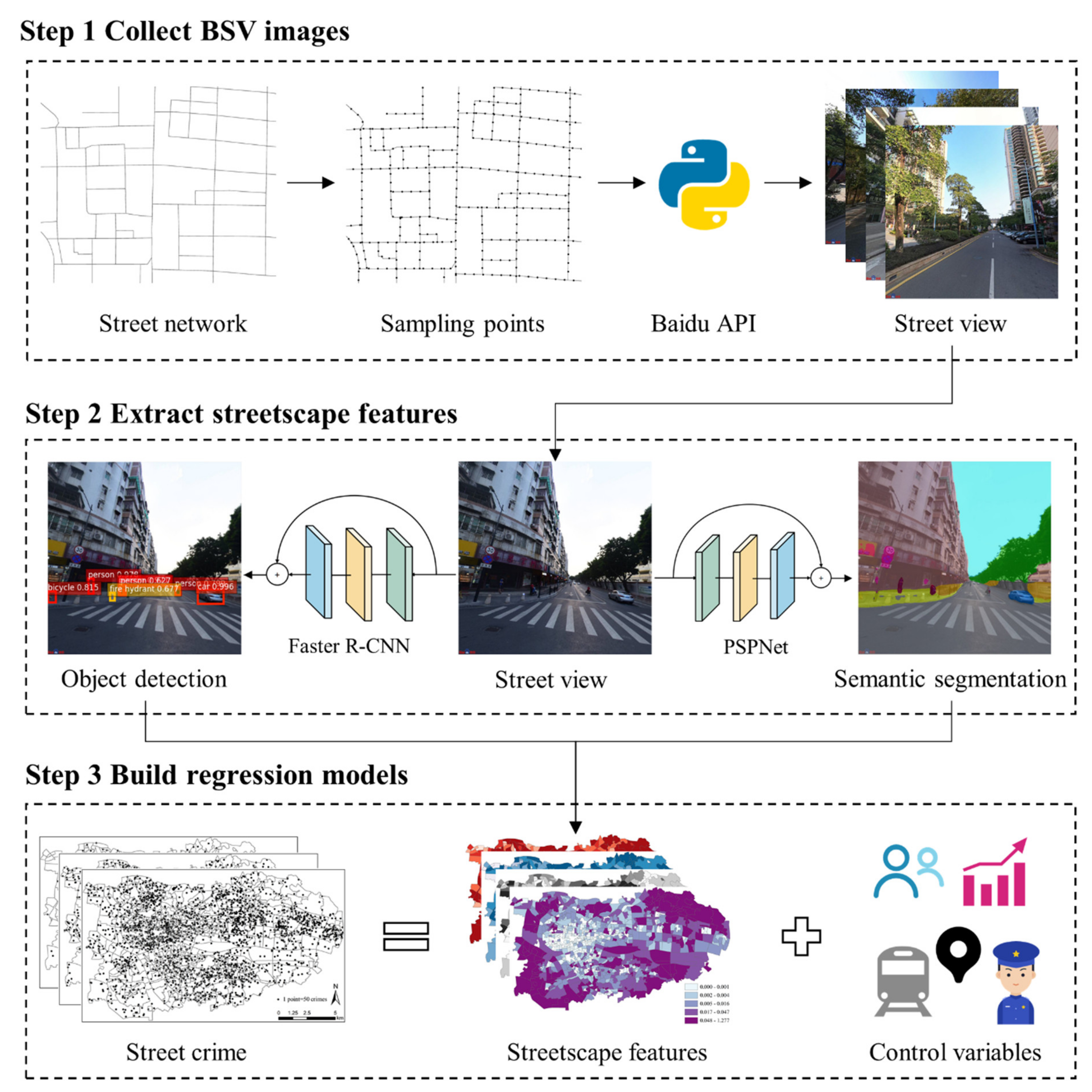
3.2.2. Collect BSV Images and Extract Streetscape Features

Compared with the human audit approach of obtaining streetscape characteristics from SVIs [5,54], emerging computer vision technologies are time-efficient and objective. We first collected fine-grained BSV images from the Baidu Map website. Then, we combined two deep learning networks to extract both people on the street and other built environment elements from BSVs and included these measures into statistical models.
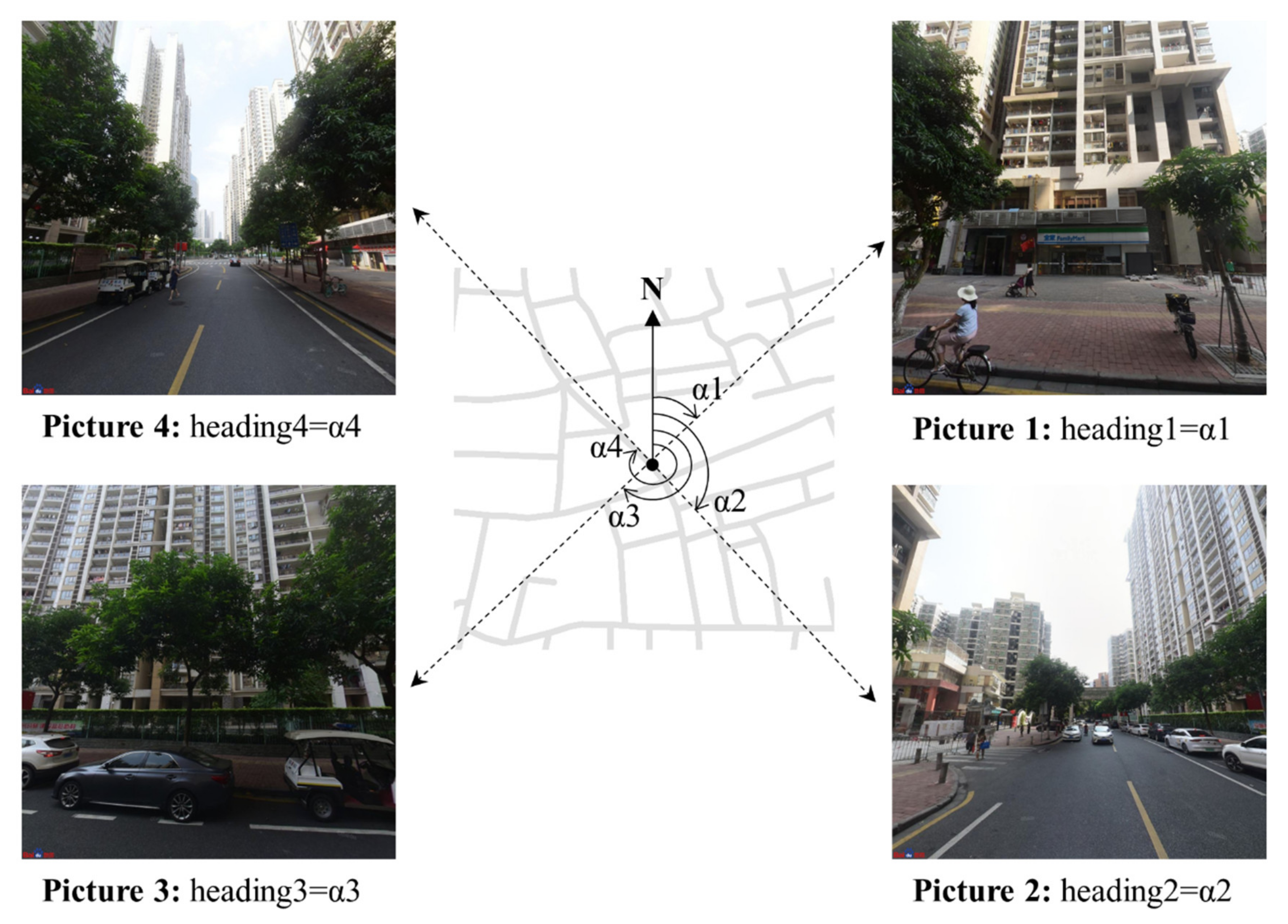
  • Fetch BSVs from the Baidu Map Website
Baidu Street View (BSV) is a map service website providing visual information on streets in more than 600 cities in China. BSV images were captured by street view cars. The key components of a street view car are a GPS and fisheye lens. The GPS is used to record geographic locations when the car is driving on the street, and the fisheye lenses are used to collect 360° street view images. The most significant advantage of street view images over other data is that they are captured by cameras set on top of cars driving along streets. Therefore, street view images can be adopted to extract street environment features from pedestrians’ views, and they have the potential to help reveal the most direct connection between streetscape conditions and crime.
We took BSV images as a proxy of the streetscape environment. Some basic information is required to collect the BSVs at a position, including the coordinates (longitude and latitude), azimuth angle (commonly called the heading angle), and pitch angle. We first generated sampling points along the street at a uniform interval of 20 m. Based on their coordinates, we collected fine-grained BSV images. There were 215,760 sample sites in the study region.
To be consistent with pedestrians’ directions of eyesight, we collected BSV images in four horizontal directions at each sample site. Two directions were parallel to the street, and two directions were vertical to the street, as demonstrated in Figure 2. The pitch angle of each image was set to 0° to meet the way people experience the street environment. We then downloaded the BSV images through the Baidu Street View API (see Baidu Developer Platform). Finally, we collected a total of 863,040 images in the study region. The metadata show that they were all captured between 2017 and 2019, consistent with the crime time. As an urbanized region, the built environment in the study area did not changed dramatically during this short period, so the time differences of the BSV images were negligible. Each BSV image had a field of view of 90°, so four images together could capture the panorama of a site.
This study translated the BSV images into meaningful factors and then incorporated them into regression models. The urban streetscape is a complex system containing components of diverse shapes and sizes. Therefore, we combined two deep learning networks to extract different and complementary information from each BSV image.
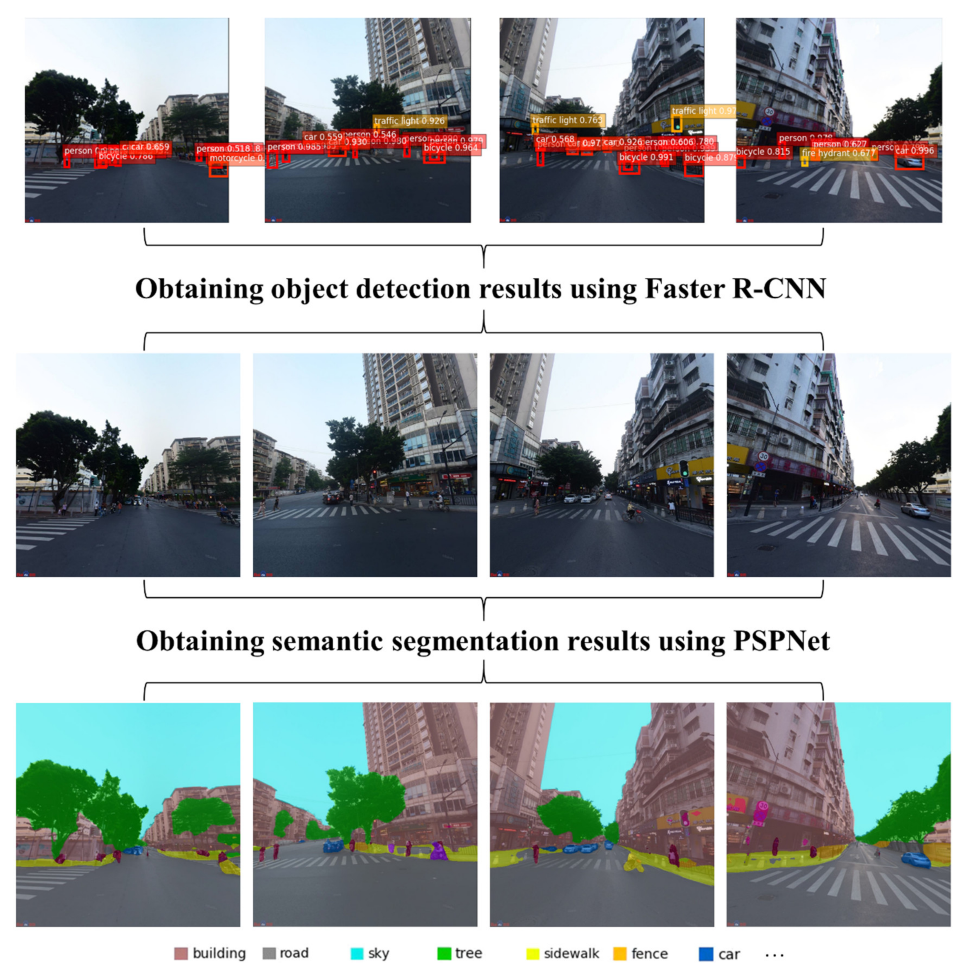
  • Object Detection Using the Faster R-CNN Network
Some objects like persons and cars are discrete elements with relatively fixed shapes and distinct outlines in an image. Therefore, it is practical to measure the count of identifiable objects. Faces and license plates are blurred in the Baidu Street View images; therefore, this study had no privacy or ethical issues. This study applied a pretrained Faster R-CNN network [55] to perform object detection for BSV images. This network was chosen because it reached a good balance between prediction accuracy and operational efficiency as a state-of-the-art deep learning network. Additionally, it was perfectly compatible with the high resolution of BSV images collected in this study (1024 × 1024 pixels).
The outputs of a Faster R-CNN network were a set of predicted bounding boxes. Each box had an associated score indicating the credibility of whether the box contained an object or not inside and a label determining which category the object belonged to. Based on the outputs of the Faster R-CNN network, we could count the number of objects in each category in an image and finally calculate their total amounts in each community.
This research retrieved the number of people on the street in a community according to the following formula:
N u m b e r   o f   p e o p l e   o n   t h e   s t r e e t = i = 1 n j = 1 4 I m a g e p _ j
where Imagep_j is the number of people in the image taken in the jth direction among the four directions at a position and n represents the total number of collecting points within a community.
The on-street population must be considered when studying street crime. However, on-street population sizes in different places are difficult to obtain. Pedestrian volume data have traditionally been collected through field observations, which has many methodological limitations, such as being time-consuming, labor-intensive, and inefficient. Various big data, such as mobile phone data, geotagged social media data, metro smart card data, and taxi and bicycle trajectory data, are incapable of capturing the movement of pedestrians. Assessing pedestrian volumes automatically from street view images with machine learning techniques can overcome such limitations, because this approach offers a broad geographic reach and consistent image acquisition. While SVIs have been recently used to estimate street-level pedestrian volumes [52,53], this approach has not been applied to crime research.
  • Semantic Segmentation Using the PSPNet Network
Unlike objects with fixed shapes and distinct outlines, sky, grass, and roads may not have a definitive shape in an image. Therefore, object detection networks are not applied to these features. This study utilized a semantic segmentation network instead. After comparing several deep learning models, we chose the widely applied Pyramid Scene Parsing Network (PSPNet) [56]. Semantic segmentation models generate pixel-wise predictions and assign each pixel a category label. We measured the proportions of these features in the image.
By borrowing ideas from the green view index calculation formula developed by Li et al. [57], which measured the proportion of vegetarians in a location, we calculated the proportion of a class of objects in a community as follows:
P r o p o r t i o n   o f   o b j e c t = i = 1 n j = 1 4 I m a g e o _ j i = 1 n j = 1 4 I m a g e t _ j 100 %
where Imageo_j is the number of pixels belonging to one type of object in the image taken in the jth direction and Imaget_j is the total number of pixels in that image, while n represents the total number of collecting points within a community.
By combining the results of object detection and the semantic segmentation networks (see Figure 3), we finally derived eight quantitative measurements of streetscape features. They were the number of people on the street (per 1000), the average proportion of paths (%), the average proportion of roads (%), the average proportion of walls (%), the average proportion of buildings (%), the number of streetlamps (per 1000), the number of traffic lights (per 1000), and the average proportion of trees (%). The rest of the object categories were not included in the analysis as they were considered irrelevant to crime in an urban context. Figure 4 presents the spatial distributions of people on the street and the streetscape physical features retrieved by BSV images and deep learning methods.

3.2.3. Control Variables

Data obtained from the Sixth Nationwide Census were used to retrieve socioeconomic and demographic factors. Land use features were extracted from Gaode Map. Based on the data provided by Daodaotong Map, we further acquired the features of surveillance and transportation facilities.
  • Socioeconomic and Demographic Factors
We collected the socioeconomic and demographic factors, including the rate of young people, the rate of highly educated people, the rate of migrant people, and the rate of renters. Young people are the main perpetrators of crimes [15], so we used young people (aged 30–45 years) to indicate possible offenders. We used the rate of highly educated people to approximate the income level, which has a specific association with crime [15,58]. Studies proved that migrants were positively related to crime by increasing instability and disrupting social order [59]. Therefore, we obtained the rate of migrant people by calculating the proportion of people whose Hukou was not in ZG city. Similarly, we considered the rate of renters, as this is also a factor adverse to residential stability and social organization [59].
  • Land Use Features
This study used the number of POIs in each community to proxy the number of point-level land uses. In addition, we calculated the mixture of POIs to measure the land use heterogeneity by the adjusted Herfindahl–Hirschman Index [60]:
M i x = 1 j = 1 J P j 2
where P j is the proportion of the number of jth type POIs. A Mix close to 1 indicates a strong land use mixture, while a Mix close to 0 indicates a weak land use mixture. Some research claimed that a mixed land use pattern could weaken the informal control of residents and increase crime [61], while some research revealed that a complex land use composition attracts people and promotes activities, thereby curbing crime by increasing social control [15,62].
  • Formal Surveillance
Police stations are the most basic level of governmental management institutions in China. They can act as a deterrent to crime [63]. This study used the number of police stations to proxy the formal surveillance levels.
  • Transportation Facilities
This study adopted two transportation facility variables to measure traffic accessibility. They were the number of bus stops and the number of subway stations. The relationship between traffic accessibility and crime is complex. Some studies demonstrated that convenient transportation could promote pedestrian activities, enhance natural surveillance, and deter crimes [15], while some studies proved that transportation facilities attract targets and act as escape routes, thus providing opportunities for offenders [34,63].
Table 1 lists the summary statistics of the dependent and independent variables used in this study.

3.3. Method

The dependent variables were community-level crime counts, which were over-dispersed nonnegative integers. Therefore, negative binomial regression models were adopted in this study to model the associations between the street view variables and the number of crimes:
l n Y i = β 0 + k = 0 k β k X i k + l = 0 l β l X i l + m = 0 m β m X i m + n = 0 n β n X i n + p = 0 p β p X i p
where Y i represents the crime count in community i, the βs are regression coefficients estimated by the model, indicating the influences of independent variables on the dependent variable, and X i k ,   X i l ,   X i m ,   X i n , and X i p are independent variables of five categories (socioeconomic and demographic factors, land use features, formal surveillance, transportation facilities, and streetscape features, respectively).
We calculated the Moran’s I indexes of the dependent variables to examine whether spatial autocorrelation effects existed. The results indicate that all three types of crime were autocorrelated in space. Therefore, we added a spatial lag into the modal as an independent variable to address the spatial autocorrelation issue. The spatial lag was calculated as follows:
L a g i = j = 1 , i j N C j N
where L a g i is the spatial lag of the dependent variable in community i, j is a neighbor of community i, N is the total number of neighbors of community i, and C j is the number of crimes in community j. In short, the spatial lag of community i measured the average crime count of its neighbors. In this study, we used the Queen adjacency criterion to determine the neighbors of community i.
Figure 5 summarizes the workflow of the study, which included three steps: (1) generating sampling points along the street, based on which fine-grained BSV images were collected using the Baidu API, (2) extracting streetscape features using an object detection method (Faster R-CNN) and a semantic segmentation method (PSPNet), and (3) building regression models to determine the influences of the on-street population and streetscape physical environment on street crime, controlling for the effects of socioeconomic and demographic factors, land use features, and surveillance and transportation facilities.

4. Results

Before running the regression models, we checked all explanatory variables’ VIF (variable inflation factor) values to check for multicollinearity. The results showed that the VIF values of all explanatory variables were much smaller than the commonly accepted threshold of 10 in crime research [64]. Therefore, the results in this study had no serious multicollinearity issues. Additionally, we standardized all explanatory variables before incorporating them into the regression models because the covariates had different units and significant disparities in magnitude. Standardization also makes it easy to compare the magnitudes of the impacts of different variables [65]. In order to assess the improvements of model performances after incorporating streetscape variables, we ran baseline models which did not contain the streetscape variables. We utilized log-likelihood and AIC to compare the model performances comprehensively. A larger log-likelihood value indicated a better model fit, while a smaller AIC value indicated a better one.
Table 2 presents the results of the spatial lag negative binomial regression estimations. Models (1, 3, and 5) are baseline models which only included the control variables, while Models (2, 4, and 6) are the full models which contained additional streetscape variables. Both the log-likelihood and AIC values demonstrated that adding street view variables improved the model fits. For total street crime, the log-likelihood of Model (2) (−3821.261) was larger than that of Model (1) (−3837.600), The AIC of Model (2) (7682.521) was smaller than that of Model (1) (7699.199). For street property crime, the log-likelihood of Model (4) (−3689.161) was larger than that of Model (3) (−3704.309), and the AIC of Model (4) (7418.322) was smaller than that of Model (3) (7432.617). For street violent crime, the log-likelihood of Model (6) (−2592.888) was larger than that of Model (5) (−2608.377), and the AIC of Model (6) (5225.775) was smaller than that of Model (5) (5240.753). Therefore, we discuss only the results of the full models in the following section.
The number of people on the street had the most considerable impact on the total street crimes and street property crimes among all the streetscape variables. Specifically, a one standard deviation increase in the number of people on the street was associated with a 7.8% (IRR = 1.078) increase in the number of total street crimes and a 7.9% (IRR = 1.079) increase in the number of street property crimes. The number of people on the street also positively influenced street violent crime, but the effect was not statistically significant. The average proportion of paths had a significant negative impact on three types of crime. A one standard deviation increase of this factor was associated with a 4.5% (IRR = 0.955) decrease in the number of total street crimes, a 4.3% (IRR = 0.957) decrease in the number of street property crimes, and a 4% (IRR = 0.960) decrease in the number of street violent crimes. Similarly, the average proportions of buildings and trees were also significantly and negatively associated with three types of crime. Specifically, a one standard deviation increase in the average proportion of buildings would result in a 5% (IRR = 0.950) decrease in the number of all street crimes, a 4.9% (IRR = 0.951) decrease in the number of street property crimes, and a 6.1% (IRR = 0.939) decrease in the number of street violent crimes. A one standard deviation increase in the average proportion of trees was associated with a 6.5% (IRR = 0.935) decrease in the number of total street crimes, a 6.5% (IRR = 0.935) decrease in the number of street property crimes, and a 7.2% (IRR = 0.928) decrease in the number of street violent crimes. The average proportion of roads and the number of traffic lights had positive relationships with the three types of crime, but these relationships did not reach statistical significance. The average proportion of walls and number of streetlamps had nonsignificant and negative correlations with the three types of crime.
As for the control variables, the rate of young people, the rate of highly educated people, the rate of renters, and the number of POIs had significantly positive associations with the three types of crime. The rate of migrant people, the mixture of POIs, and the number of bus stops had positive relationships with the three types of crime, but the effects were not significant. The number of subway stations had a significant negative association with street violent crime, and its correlations with the other two types of crime were insignificant. The number of police stations had negative associations with the three types of crime, but the effects were insignificant.
The spatial lags of the dependent variables had significant and solid positive associations with the numbers of all types of crime, revealing the spatial autocorrelation effect of crime events. Therefore, the spatial lag models used in this study were valid.
We used the k-fold cross-validation technique to validate the regression models used in this study. This technique first divides the total dataset into k parts of equal size, iteratively excludes one part (called the validation set) at a time, and predicts it with the parts not excluded (called the training set). At each step, an R2 score can be calculated, measuring the prediction accuracy of the trained model. Figure 6 presents the results of the cross-validation R2 score when k was set at different values. When k reached about 30 and above, the performance of the three models became stable, with the R2 score reaching above 0.8, indicating that the models in this study were sufficiently accurate.

5. Discussion

Overall, the findings of this research are consistent with the previous literature. The number of people on the street had different effects on different types of crime. The total street crime and street property crime had significant positive associations with the number of people on the street, indicating that places with more people on the street have higher risks for total street crime and street property crime. Although the number of people on the street also positively influenced street violent crime, this effect was not significant statistically (p = 0.128). Therefore, street violent crime in a place would not witness a remarkable change in the number of people on the street. Such a disparity advocates for previous theoretical and empirical studies. First, both crime pattern theory and routine activity theory argue that offenders make rational decisions by balancing the potential benefits, costs, and risks when committing a crime. In general, offenders tend to commit crimes where suitable targets are present and capable guardians are absent. However, each type of crime has unique choice-structuring properties [66]. The influence of the presence of people in a given area is mainly dependent upon the nature of the crime; that is, the presence of people has diverse impacts on different types of crime [23]. Street property crimes, such as snatching, pickpocketing, and theft, have the nature of concealment and transience. Property crime offenders prefer to “fish in troubled waters” in that they usually commit crimes in crowded places when people are not paying attention and then flee the scene quickly. The whole process of committing a crime must be completed rapidly without being noticed. A thick crowd of people in a location not only offers a lot of targets and opportunities, but the presence of a dense population can also provide perfect cover for the whole process of a crime: looking for a target, committing a crime, and fleeing the scene after a crime. This makes streets with dense populations ideal places for property crime. This is proven by the fact that property crimes have high exposure rates and low detection rates [31]. However, street violent crimes such as robbery, intentional injury, and assault do not happen secretly but usually with sounds of a struggle, making it easy to be spotted and draw people’s attention. Therefore, these types of crimes are unlikely to happen in crowded places. Social disorganization theory focuses on the static of the residential population rather than the environment or the simple magnitude of floating populations [21]. The theory highlights that the local characteristics in a location improve individual tendencies toward delinquent behaviors or hinder collective efforts to preserve public order.
Second, the inconsistent influences of people on the street on different types of crime were also found in previous empirical studies. For example, Vomfell et al. utilized Twitter and taxi data to help forecast crime [24]. They concluded that using these features can significantly improve the prediction accuracy of property crime. For violent crime, however, the spatiotemporal dimension of these features adds very little value. They further explained that long-term neighborhood structural conditions are the primary influences of violent crime. Social deprivation, for example, provides the context for violent behaviors. Therefore, violent crimes commonly take place in locations with poor social cohesion. As for property crime, it is local opportunities through anonymity that matter, rather than deprivation. Another study conducted by Malleson and Andresen in Leeds found similar results; although the study region had a large volume of violent crimes, there was no statistically significant elevation in the risk of violent criminal victimization when considering a theoretically informed population at risk [47].
The physical environment variables deduced from BSV images also had meaningful associations with street crime. The average proportion of trees had the most significant influence on all types of crime among the street view variables. Specifically, the impacts were all significantly negative. Therefore, places with higher eye-level street green spaces were associated with less crime. Green spaces have been proven to improve community cohesion, making people’s desire to survey their surroundings and intervene in an ongoing crime stronger [67,68]. Well-maintained vegetation in a place can also act as a cue to care, indicating that inhabitants actively care about their territory and potentially suggesting that an intruder would be noticed and confronted [69]. Additionally, green spaces, including trees, parks, and other natural features, could play a relieving effect that can make human psychological and emotional states calm, improve cognitive functioning, and inhibit people from committing crimes [70,71]. A series of empirical research has proven green spaces to be inhabitable to crime [7,67,68,69,70,71,72].
The average proportion of paths was also negatively associated with all three types of crime, and the effects were statistically significant. This result supports the previous advocation of adopting design principles that facilitate walking and social interaction, because human activity could help promote a sense of community belonging, which is beneficial for crime prevention [73]. Places with high proportions of paths provide spaces for outdoor activity. People living here are more likely to go out and associate with others. Therefore, people’s anonymity decreases, as there is an opportunity to gain mutual acquaintance with other residents, enabling social control of inhibiting crime because unfamiliar people will stand out as strangers in these neighborhoods.
The average proportion of buildings had significantly negative associations with all three types of crime. As shown in Figure 4e, communities with high average proportions of buildings are generally dispersed along arterial roads. Buildings extracted from GSVs in these areas are usually high-rise buildings fronting the street, indicating these districts are work areas with many employees. Jacobs assumed that such vibrant locations would have less crime given the presence of many guardians [74]. A similar study about the associations between the built environment and crime using GSV images demonstrated that the presence of buildings was generally unrelated to crime, except for robberies [10].
Other street view variables such as the average proportion of roads, the average proportion of walls, number of streetlamps, and number of traffic lights had no statistically significant relationships with any of the three types of crime. Therefore, we do not discuss these variables further.
The spatial lags of the dependent variables significantly impacted all types of crime. Specifically, according to the results of the full models, a one standard deviation increase in the spatial lag of the dependent variable was associated with an 85.1% (IRR = 1.851) increase in the number of total street crimes, an 88.2% (IRR = 1.882) increase in the number of street property crimes, and a 93.9% (IRR = 1.939) increase in the number of street violent crimes. These results reveal the widely existing spatial autocorrelation effect of geographic events. Modeling crime using a spatial regression model is thus necessary.

6. Conclusions

The presence and size of people on the street and physical streetscape characteristics have close associations with criminal activities [7,8,75]. However, large-scale environment conditions, especially fine-grained streetscape features, are difficult or expensive to obtain. The absence of precise quantitative data for street scenes leaves the relationship between crime and the visual characteristics of a streetscape unrevealed [76,77]. This study integrated BSV images and deep learning methods to retrieve detailed and rich information about the streetscape context. Controlling for the spatial autocorrelation effect, we constructed spatial lag negative binomial regression models to evaluate the influences of people on the street and the streetscape physical features on crime.
The results of this study are promising. First, the significant improvements in model performance after incorporating the street view variables demonstrate the necessity for accounting for the effect of the streetscape context when studying crime. Second, the number of people on the street had significant positive impacts on the total street crime and street property crime. However, no significant impacts were found on street violent crime. Therefore, the effect of human presence on crime is greatly determined by the nature of the crime. The phenomenon that the same street view variable had different effects on different types of crime reveals that the study of the general type of crime is insufficient. It ignores the different occurrence mechanisms of different types of crime. Third, regarding the physical streetscape features, the average proportion of paths, buildings, and trees had statistically significant and negative impacts on both the occurrence of street property crime and street violent crime.
This study is the first attempt at combining street view images and deep learning algorithms to extract both the on-street population and a series of eye-level physical streetscape features to investigate street crime. Previous studies could not distinguish between the street and indoor populations, and they were potentially biased by counting indoor people for their possible influence on street crime. This study provides evidence that streetscape features, including people on the street retrieved from street view images, can effectively explain street crime. The available street view images provide new opportunities for gathering large-scale quantitative streetscape characteristics which provide a basis for place-based crime research.
The presence of people on the street is a prerequisite for the occurrence of a street crime. Therefore, the on-street population is an essential factor of street crime. Traditional field observation methods used to collect the pedestrian volume are time-consuming, labor-intensive, and inefficient, while big data sources like mobile phone data, geotagged social media data, metro smart card data, and taxi and bicycle trajectory data are incapable of capturing the movement of pedestrians. Such limitations can be overcome by the method used in this study. Assessing the pedestrian volume automatically from street view images with deep learning techniques is a reliable method for determining the on-street population size. The availability of street view images offers broad geographic coverage. The methods utilized in this study could be applied to street crime research in other countries and regions. Researchers from other fields, such as public health, urban vitality, and street design, could also borrow ideas from this study, because the on-street population and streetscape features are important in these fields.
This study’s findings not only validate criminology theories but also have implications for crime prevention and urban planning. Trees have a significantly negative impact on street crime. Therefore, urban designers may improve the environment by planting trees. Paths are also a design element found to have a crime deterring effect. Therefore, this design principle can be adopted to create spaces for outdoor activity. Police patrols should be deployed in targeted areas with high proportions of young people and renters. Furthermore, although communities with more POIs promote vitality and have other advantages, they may also have some unexpected drawbacks, such as street crime.
Several limitations of this research should be noted and addressed in the future. First, although the street view image is a valuable and accessible data source for determining the on-street population size, most street view images were captured in the daytime. Therefore, it cannot be known what the population size on the street was in the evening. Future studies could use satellite night light data to proxy on-street populations in the evening, as facilities are typically associated with lights at night [78]. Second, some objects such as litter, graffiti, broken windows, and property damage are not easily detected using existing methods. These objects are signs of physical incivilities, which have been demonstrated to attract crimes. Future studies could collect such fine-scale quantitative data using the environmental audit approach [5]. Third, apart from the physical environment, human visual perception of the urban environment can also affect the occurrence of crimes. Therefore, future research could account for perception [50].

Author Contributions

Conceptualization, Han Yue and Lin Liu; methodology, Han Yue, Huafang Xie and Jianguo Chen; writing—original draft preparation, Han Yue and Huafang Xie; writing—review and editing, Lin Liu and Jianguo Chen. All authors have read and agreed to the published version of the manuscript.

Funding

This research was partially supported by the National Key Research and Development Program of China No. 2018YFB0505500 and 2018YFB0505503.

Data Availability Statement

Not available.

Acknowledgments

The authors are very grateful for the comments of the reviewers and the editor, which have helped improve the article considerably.

Conflicts of Interest

The authors declare no conflict of interest.

References

  1. Cohen, L.; Felson, M. Social change and crime rate trends: A routine activity approach. Am. Sociol. Rev. 1979, 44, 588–608. [Google Scholar] [CrossRef]
  2. Brantingham, P.L.; Brantingham, P.J. A theoretical model of crime hot spot generation. Stud. Crime Crime Prev. 1999, 8, 7–26. [Google Scholar]
  3. Weisburd, D. From criminals to criminal contexts: Reorienting criminal justice research and policy. Adv. Criminol. Theory 2002, 10, 197–216. [Google Scholar]
  4. Cozens, P.; Davies, T. Crime and residential security shutters in an Australian suburb: Exploring perceptions of ‘eyes on the street’, social interaction and personal safety. Crime Prev. Community Saf. 2013, 15, 175–191. [Google Scholar] [CrossRef] [Green Version]
  5. He, L.; Páez, A.; Liu, D. Built environment and violent crime: An environmental audit approach using Google Street View. Comput. Environ. Urban Syst. 2017, 66, 83–95. [Google Scholar] [CrossRef]
  6. Rundle, A.G.; Bader, M.D.M.; Richards, C.A.; Neckerman, K.M.; Teitler, J.O. Using google street view to audit neighborhood environments. Am. J. Prev. Med. 2011, 40, 94–100. [Google Scholar] [CrossRef] [Green Version]
  7. Wolfe, M.K.; Mennis, J. Does vegetation encourage or suppress urban crime? Evidence from Philadelphia, PA. Landsc. Urban Plan. 2012, 108, 112–122. [Google Scholar] [CrossRef]
  8. Zhou, H.; Liu, L.; Lan, M.; Yang, B.; Wang, Z. Assessing the Impact of Nightlight Gradients on Street Robbery and Burglary in Cincinnati of Ohio State, USA. Remote Sens. 2019, 11, 1958. [Google Scholar] [CrossRef] [Green Version]
  9. Patino, J.E.; Duque, J.C.; Pardo-Pascual, J.E.; Ruiz, L.A. Using remote sensing to assess the relationship between crime and the urban layout. Appl. Geogr. 2014, 55, 48–60. [Google Scholar] [CrossRef]
  10. Hipp, J.R.; Lee, S.; Ki, D.; Kim, J.H. Measuring the Built Environment with Google Street View and Machine Learning: Consequences for Crime on Street Segments. J. Quant. Criminol. 2021, 1–29. [Google Scholar] [CrossRef]
  11. Amiruzzaman, M.; Curtis, A.; Zhao, Y.; Jamonnak, S.; Ye, X. Classifying crime places by neighborhood visual appearance and police geonarratives: A machine learning approach. J. Comput. Soc. Sci. 2021, 4, 813–837. [Google Scholar] [CrossRef] [PubMed]
  12. Khorshidi, S.; Carter, J.; Mohler, G.; Tita, G. Explaining Crime Diversity with Google Street View. J. Quant. Criminol. 2021, 37, 361–391. [Google Scholar] [CrossRef]
  13. Zhou, H.; Liu, L.; Lan, M.; Zhu, W.; Song, G.; Jing, F.; Zhong, Y.; Su, Z.; Gu, X. Using Google Street View imagery to capture micro built environment characteristics in drug places, compared with street robbery. Comput. Environ. Urban Syst. 2021, 88, 101631. [Google Scholar] [CrossRef]
  14. Zhang, F.; Fan, Z.; Kang, Y.; Hu, Y.; Ratti, C. “Perception bias”: Deciphering a mismatch between urban crime and perception of safety. Landsc. Urban Plan. 2021, 207, 104003. [Google Scholar] [CrossRef]
  15. Yue, H.; Zhu, X. The influence of urban built environment on residential burglary in China: Testing the encounter and enclosure hypotheses. Criminol. Crim. Justice 2019, 21, 508–528. [Google Scholar] [CrossRef]
  16. Clarke, R.V.; Felson, M. Routine Activity and Rational Choice; Transaction: New Brunswick, NJ, USA, 1993. [Google Scholar]
  17. Roncek, D.W.; Bell, R. Bars, blocks, and crimes. J. Environ. Syst. 1981, 11, 35–47. [Google Scholar] [CrossRef]
  18. McCord, E.S.; Ratcliffe, J.H. Intensity value analysis and the criminogenic effects of land use features on local crime patterns. Crime Patterns Anal. 2009, 2, 17–30. [Google Scholar]
  19. Groff, E.; Mccord, E.S. The role of neighborhood parks as crime generators. Secur. J. 2012, 25, 1–24. [Google Scholar] [CrossRef]
  20. Kubrin, C.E.; Squires, G.D.; Graves, S.M.; Ousey, G.C. Does fringe banking exacerbate neighborhood crime rates? Criminol. Public Policy 2011, 10, 437–466. [Google Scholar] [CrossRef]
  21. Jung, Y.; Chun, Y.; Kim, K. Modeling Crime Density with Population Dynamics in Space and Time: An Application of Assault in Gangnam, South Korea. Crime Delinq. 2020, 68, 253–283. [Google Scholar] [CrossRef]
  22. Caminha, C.; Furtado, V.; Pequeno, T.H.C.; Ponte, C.; Melo, H.P.M.; Oliveira, E.A.; Andrade, J.S. Human mobility in large cities as a proxy for crime. PLoS ONE 2017, 12, e0171609. [Google Scholar] [CrossRef] [PubMed] [Green Version]
  23. Boivin, R. Routine activity, population(s) and crime: Spatial heterogeneity and conflicting Propositions about the neighborhood crime-population link. Appl. Geogr. 2018, 95, 79–87. [Google Scholar] [CrossRef]
  24. Vomfell, L.; Härdle, W.K.; Lessmann, S. Improving crime count forecasts using Twitter and taxi data. Decis. Support Syst. 2018, 113, 73–85. [Google Scholar] [CrossRef]
  25. Felson, M.; Eckert, M. Crime and Everyday Life, 5th ed.; Sage: Thousand Oaks, CA, USA, 2015. [Google Scholar]
  26. Song, G.; Liu, L.; Bernasco, W.; Xiao, L.; Zhou, S.; Liao, W. Testing indicators of risk populations for theft from the person across space and time: The significance of mobility and outdoor activity. Ann. Am. Assoc. Geogr. 2018, 108, 1370–1388. [Google Scholar] [CrossRef]
  27. Wilcox, P.; Land, K.C.; Hunt, S.A. Criminal Circumstance: A Dynamic, Multi-Contextual Criminal Opportunity Theory; Aldine de Gruyter: New York, NY, USA, 2003. [Google Scholar]
  28. Brantingham, P.L.; Brantingham, P.J. Crime Pattern Theory. In Environmental Criminology and Crime Analysis; Wortley, R., Mazerolle, L., Eds.; Willan Publishing: Portland, OR, USA, 2008. [Google Scholar]
  29. Nee, C.; Taylor, M. Examining burglars’ target selection: Interview, experiment or ethnomethodology? Psychol. Crime Law 2000, 6, 45–59. [Google Scholar] [CrossRef]
  30. Mayhew, P. Defensible space: The current status of a crime prevention theory. Howard J. Crim. Justice 1979, 18, 150–159. [Google Scholar] [CrossRef]
  31. Yue, H.; Zhu, X.; Ye, X.; Guo, W. The Local Colocation Patterns of Crime and Land-Use Features in Wuhan, China. ISPRS Int. J. Geo-Inf. 2017, 6, 307. [Google Scholar] [CrossRef] [Green Version]
  32. Jones, H.R. Crime and the Urban Environment; Avebury: Brookfield, VT, USA, 1993. [Google Scholar]
  33. Shu, C.-F. Housing layout and crime vulnerability. Urban Des. Int. 2000, 5, 177–188. [Google Scholar]
  34. Yue, H.; Zhu, X.; Ye, X.; Hu, T.; Kudva, S. Modelling the effects of street permeability on burglary in Wuhan, China. Appl. Geogr. 2018, 98, 177–183. [Google Scholar] [CrossRef]
  35. Hillier, B. Can streets be made safe? Urban Des. Int. 2004, 9, 31–45. [Google Scholar] [CrossRef]
  36. Skogan, W.G.; Maxfield, M.G. Coping with Crime: Individual and Neighborhood Reactions; Sage Publications: Beverley Hills, CA, USA, 1981. [Google Scholar]
  37. Walker, B.B.; Schuurman, N. The pen or the sword: A situated spatial analysis of graffiti and violent injury in Vancouver, British Columbia. Prof. Geogr. 2015, 67, 608–619. [Google Scholar] [CrossRef]
  38. Spelman, W. Abandoned buildings: Magnets for crime? J. Crim. Justice 1993, 21, 481–495. [Google Scholar] [CrossRef]
  39. Russo, S.; Roccato, M.; Vieno, A. Criminal victimization and crime risk perception: A multilevel longitudinal study. Soc. Indic. Res. 2013, 112, 535–548. [Google Scholar] [CrossRef]
  40. Andresen, M.A.; Jenion, G.W. Ambient populations and the calculation of crime rates and risk. Secur. J. 2008, 23, 114–133. [Google Scholar] [CrossRef]
  41. Panigutti, C.; Tizzoni, M.; Bajardi, P.; Smoreda, Z.; Colizza, V. Assessing the use of mobile phone data to describe recurrent mobility patterns in spatial epidemic models. R. Soc. Open Sci. 2017, 4, 160950. [Google Scholar] [CrossRef] [Green Version]
  42. Mburu, L.W.; Helbich, M. Crime Risk Estimation with a Commuter-Harmonized Ambient Population. Ann. Am. Assoc. Geogr. 2016, 106, 804–818. [Google Scholar] [CrossRef]
  43. Hipp, J.R.; Bates, C.; Lichman, M.; Smyth, P. Using Social Media to Measure Temporal Ambient Population: Does it Help Explain Local Crime Rates? Justice Q. 2018, 36, 718–748. [Google Scholar] [CrossRef] [Green Version]
  44. Tucker, R.; O’Brien, D.T.; Ciomek, A.; Castro, E.; Wang, Q.; Phillips, N.E. Who ‘Tweets’ Where and When, and How Does it Help Understand Crime Rates at Places? Measuring the Presence of Tourists and Commuters in Ambient Populations. J. Quant. Criminol. 2021, 37, 333–359. [Google Scholar] [CrossRef]
  45. Johnson, P.; Andresen, M.A.; Malleson, N. Cell Towers and the Ambient Population: A Spatial Analysis of Disaggregated Property Crime. Eur. J. Crim. Policy Res. 2020, 27, 313–333. [Google Scholar] [CrossRef]
  46. Hanaoka, K. New insights on relationships between street crimes and ambient population: Use of hourly population data estimated from mobile phone users’ locations. Environ. Plan. B Urban Anal. City Sci. 2016, 45, 295–311. [Google Scholar] [CrossRef]
  47. Malleson, N.; Andresen, M.A. The impact of using social media data in crime rate calculations: Shifting hot spots and changing spatial patterns. Cartogr. Geogr. Inf. Sci. 2014, 42, 112–121. [Google Scholar] [CrossRef]
  48. Algahtany, M.; Kumar, L. A Method for Exploring the Link between Urban Area Expansion over Time and the Opportunity for Crime in Saudi Arabia. Remote Sens. 2016, 8, 863. [Google Scholar] [CrossRef]
  49. Zhang, F.; Zhang, D.; Liu, Y.; Lin, H. Representing place locales using scene elements. Comput. Environ. Urban Syst. 2018, 71, 153–164. [Google Scholar] [CrossRef]
  50. Naik, N.; Philipoom, J.; Raskar, R.; Hidalgo, C. Streetscore—Predicting the perceived safety of one million streetscapes. In Proceedings of the IEEE Conference on Computer Vision and Pattern Recognition Workshops, Columbus, OH, USA, 23–28 June 2014. [Google Scholar]
  51. Jiang, Y.; Chen, L.; Grekousis, G.; Xiao, Y.; Ye, Y.; Lu, Y. Spatial disparity of individual and collective walking behaviors: A new theoretical framework. Transp. Res. Part D Transp. Environ. 2021, 101, 103096. [Google Scholar] [CrossRef]
  52. Chen, L.; Lu, Y.; Sheng, Q.; Ye, Y.; Wang, R.; Liu, Y. Estimating pedestrian volume using Street View images: A large-scale validation test. Comput. Environ. Urban Syst. 2020, 81, 101481. [Google Scholar] [CrossRef]
  53. Yin, L.; Cheng, Q.; Wang, Z.; Shao, Z. ‘Big data’ for pedestrian volume: Exploring the use of Google Street View images for pedestrian counts. Appl. Geogr. 2015, 63, 337–345. [Google Scholar] [CrossRef]
  54. Sytsma, V.A.; Connealy, N.; Piza, E.L. Environmental Predictors of a Drug Offender Crime Script: A Systematic Social Observation of Google Street View Images and CCTV Footage. Crime Delinq. 2020, 67, 27–57. [Google Scholar] [CrossRef]
  55. Ren, S.; He, K.; Girshick, R.; Sun, J. Faster r-cnn: Towards real-time object detection with region proposal networks. Adv. Neural Inf. Processing Syst. 2015, 28, 91–99. [Google Scholar] [CrossRef] [Green Version]
  56. Zhao, H.; Shi, J.; Qi, X.; Wang, X.; Jia, J. Pyramid scene parsing network. In Proceedings of the IEEE Conference on Computer Vision and Pattern Recognition (CVPR), Honolulu, HI, USA, 21–26 July 2017; pp. 2881–2890. [Google Scholar]
  57. Li, X.; Zhang, C.; Li, W.; Ricard, R.; Meng, Q.; Zhang, W. Assessing street-level urban greenery using Google Street View and a modified green view index. Urban For. Urban Green. 2015, 14, 675–685. [Google Scholar] [CrossRef]
  58. Wu, L.; Liu, X.; Ye, X.; Leipnik, M.; Lee, J.; Zhu, X. Permeability, space syntax, and the patterning of residential burglaries in urban China. Appl. Geogr. 2015, 60, 261–265. [Google Scholar] [CrossRef]
  59. Du, F.; Liu, L.; Jiang, C.; Long, D.; Lan, M. Discerning the Effects of Rural to Urban Migrants on Burglaries in ZG City with Structural Equation Modeling. Sustainability 2019, 11, 561. [Google Scholar] [CrossRef] [Green Version]
  60. He, Q.; Li, J. The roles of built environment and social disadvantage on the geography of property crime. Cities 2022, 121, 103471. [Google Scholar] [CrossRef]
  61. Kurtz, E.M.; Koons, B.A.; Taylor, R.B. Land use, physical deterioration, resident-based control, and calls for service on urban streetblocks. Justice Q. 2006, 15, 121–149. [Google Scholar] [CrossRef]
  62. Kim, Y.-A.; Hipp, J.R. Density, diversity, and design: Three measures of the built environment and the spatial patterns of crime in street segments. J. Crim. Justice 2021, 77, 101864. [Google Scholar] [CrossRef]
  63. Chen, J.G.; Liu, L.; Xiao, L.Z.; Xu, C.; Long, D.P. Integrative Analysis of Spatial Heterogeneity and Overdispersion of Crime with a Geographically Weighted Negative Binomial Model. ISPRS Int. J. Geo-Inf. 2020, 9, 60. [Google Scholar] [CrossRef] [Green Version]
  64. Bernasco, W.; Block, R. Robberies in Chicago: A block-level analysis of the influence of crime generators, crime attractors, and offender anchor points. J. Res. Crime Delinq. 2011, 48, 33–57. [Google Scholar] [CrossRef]
  65. Fotheringham, A.S.; Yue, H.; Li, Z. Examining the influences of air quality in China’s cities using multi—Scale geographically weighted regression. Trans. GIS 2019, 23, 1444–1464. [Google Scholar] [CrossRef]
  66. Cornish, D.B.; Clarke, R.V. Understanding crime displacement: An application of rational choice theory. Criminology 1987, 25, 933–947. [Google Scholar] [CrossRef]
  67. Bogar, S.; Beyer, K.M. Green Space, Violence, and Crime: A Systematic Review. Trauma Violence Abus. 2016, 17, 160–171. [Google Scholar] [CrossRef]
  68. Blair, L. Community Gardens and Crime: Exploring the Roles of Criminal Opportunity and Informal Social Control; University of Cincinnati: Cincinnati, OH, USA, 2014. [Google Scholar]
  69. Kuo, F.E.; Sullivan, W.C. Environment and Crime in the Inner City. Environ. Behav. 2016, 33, 343–367. [Google Scholar] [CrossRef] [Green Version]
  70. Lin, B.B.; Egerer, M.H.; Ossola, A. Urban Gardens as a Space to Engender Biophilia: Evidence and Ways Forward. Front. Built Environ. 2018, 4, 4. [Google Scholar] [CrossRef] [Green Version]
  71. Roe, J.J.; Thompson, C.W.; Aspinall, P.A.; Brewer, M.J.; Duff, E.I.; Miller, D.; Mitchell, R.; Clow, A. Green space and stress: Evidence from cortisol measures in deprived urban communities. Int. J. Environ. Res. Public Health 2013, 10, 4086–4103. [Google Scholar] [CrossRef] [PubMed] [Green Version]
  72. Garvin, E.C.; Cannuscio, C.C.; Branas, C.C. Greening vacant lots to reduce violent crime: A randomised controlled trial. Inj. Prev. 2013, 19, 198–203. [Google Scholar] [CrossRef] [PubMed]
  73. Talen, E. Charter of the New Urbanism; McGraw Hill Education: New York, NY, USA, 2013. [Google Scholar]
  74. Jacobs, J. The Death and Life of Great American Cities; Random House: New York, NY, USA, 1961. [Google Scholar]
  75. Chalfin, A.; Hansen, B.; Lerner, J.; Parker, L. Reducing Crime Through Environmental Design: Evidence from a Randomized Experiment of Street Lighting in New York City. J. Quant. Criminol. 2021, 1–31. [Google Scholar] [CrossRef]
  76. Barnum, J.D.; Caplan, J.M.; Kennedy, L.W.; Piza, E.L. The crime kaleidoscope: A cross-jurisdictional analysis of place features and crime in three urban environments. Appl. Geogr. 2017, 79, 203–211. [Google Scholar] [CrossRef] [Green Version]
  77. Lee, I.; Jung, S.; Lee, J.; Macdonald, E. Street crime prediction model based on the physical characteristics of a streetscape: Analysis of streets in low-rise housing areas in South Korea. Environ. Plan. B Urban Anal. City Sci. 2017, 46, 862–879. [Google Scholar] [CrossRef]
  78. Liu, L.; Zhou, H.; Lan, M. Agglomerative Effects of Crime Attractors and Generators on Street Robbery? An Assessment by Luojia 1-01 Satellite Nightlight. Ann. Am. Assoc. Geogr. 2021, 112, 350–367. [Google Scholar] [CrossRef]
Figure 1. Dot density maps showing spatial distribution of the number of (ac) in the study area as of 2017–2019. Dots were randomly placed in a polygon.
Ijgi 11 00151 g001
Figure 2. An example of calculating heading angles of four BSV images at a sample site. Heading angles of Pictures 2 and 4 are parallel to the street, capturing the front and rear views, while heading angles of Pictures 1 and 3 are vertical to the street, capturing the left-hand and right-hand views.
Ijgi 11 00151 g002
Figure 3. Obtaining object detection and semantic segmentation results of BSV images via Faster RCNN and PSPNet networks.
Ijgi 11 00151 g003
Figure 4. Spatial distributions of people on the street and streetscape physical features retrieved by BSV images and deep learning methods.
Ijgi 11 00151 g004
Figure 5. Workflow of this study.
Ijgi 11 00151 g005
Figure 6. Cross-validation R2 score of different fractions of training data for the regression models.
Ijgi 11 00151 g006
Table 1. Summary statistics of dependent and independent variables.
VariableMeanSDMinMax
Dependent Variables
Number of total street crimes155.28183.7951952
Number of street property crimes126.53155.6731808
Number of street violent crimes28.7534.400306
Control Variables
Rate of young people (%)26.5345.9084.65447.431
Rate of highly educated people (%)14.31612.5650.000 86.245
Rate of migrant people (%)42.23521.4940.20398.518
Rate of renters (%)30.63623.4410.000 100.000
Number of POI (per 1000)0.3230.2830.0042.451
Mixture of POI0.826 0.074 0.341 0.904
Number of bus stops1.7692.121015
Number of subway stations0.1110.35103
Number of police stations1.3841.524010
Streetscape Variables
Number of people on the street (per 1000)1.1761.0480.0437.097
Average proportion of paths (%)0.0370.0860.000 1.276
Average proportion of roads (%)18.9393.4785.29928.953
Average proportion of walls (%)3.1312.2960.08521.107
Average proportion of buildings (%)26.218 8.753 4.166 55.116
Number of streetlamps (per 1000)0.4300.7110.0147.280
Number of traffic lights (per 1000)0.0380.04200.377
Average proportion of trees (%)17.6116.7051.51939.980
Table 2. Results of spatial lag negative binomial regression models with all independent variables standardized.
Dep. Var.Total Street CrimeStreet Property CrimeStreet Violent Crime
Model(1)
IRR
(Std. Err.)
(2)
IRR
(Std. Err.)
(3)
IRR
(Std. Err.)
(4)
IRR
(Std. Err.)
(5)
IRR
(Std. Err.)
(6)
IRR
(Std. Err.)
Control Variables
Rate of young people1.046 **1.038 **1.04 **1.032 *1.08 ***1.073 ***
(0.019)(0.019)(0.02)(0.019)(0.02)(0.020)
Rate of highly educated people1.040 **1.062 ***1.04 *1.059 ***1.06 ***1.069 ***
(0.019)(0.021)(0.02)(0.021)(0.02)(0.021)
Rate of migrant people1.0321.0241.031.0191.04 *1.028
(0.021)(0.021)(0.02)(0.022)(0.02)(0.022)
Rate of renters1.087 ***1.086 ***1.09 ***1.091 ***1.05 **1.055 **
(0.023)(0.024)(0.02)(0.024)(0.02)(0.023)
Number of POIs1.188 ***1.162 ***1.20 ***1.166 ***1.10 ***1.088 ***
(0.033)(0.033)(0.03)(0.034)(0.03)(0.029)
Mixture of POIs1.0151.0271.011.0251.001.013
(0.018)(0.018)(0.02)(0.019)(0.02)(0.019)
Number of subway stations1.0051.0001.011.0050.970.963 **
(0.018)(0.018)(0.02)(0.018)(0.02)(0.017)
Number of bus stops1.034 *1.0041.03 *1.0051.04 **1.014
(0.020)(0.023)(0.02)(0.024)(0.02)(0.024)
Number of police stations0.9840.9870.990.9890.970.979
(0.016)(0.016)(0.02)(0.017)(0.02)(0.017)
Streetscape Variables
Number of people on the street 1.078 *** 1.079 *** 1.042
(0.029) (0.030) (0.028)
The average proportion of paths 0.955 ** 0.957 ** 0.960 *
(0.019) (0.020) (0.021)
The average proportion of roads 1.019 1.015 1.037
(0.024) (0.025) (0.026)
The average proportion of walls 0.979 0.975 0.997
(0.021) (0.021) (0.022)
The average proportion of buildings 0.950 * 0.951 * 0.939 **
(0.028) (0.029) (0.029)
Number of streetlamps 0.962 0.957 0.982
(0.028) (0.029) (0.029)
Number of traffic lights 1.042 1.047 1.019
(0.029) (0.030) (0.029)
The average proportion of trees 0.935 *** 0.935 ** 0.928 ***
(0.024) (0.024) (0.025)
Spatial lag of dependent variable1.918 ***1.851 ***1.946 ***1.882 ***1.997 ***1.939 ***
(0.064)(0.061)(0.068)(0.065)(0.056)(0.054)
Log-likelihood−3837.600−3821.261−3704.309−3689.161−2608.377−2592.888
AIC7699.1997682.5217432.6177418.3225240.7535225.775
Note: The dependent variables are the number of total street crimes, number of street property crimes, and number of street violent crimes. IRR = incidence rate ratio. ***, **, and * indicate significance at the 1%, 5%, and 10% levels, respectively. In parentheses, the standard errors are given. The intercept terms are not listed. The likelihood ratio test of α = 0 demonstrates that negative binomial models are more suitable than standard Poisson models (p < 0.001).
Publisher’s Note: MDPI stays neutral with regard to jurisdictional claims in published maps and institutional affiliations.

