
Comparative Study on Matching Methods for the Distinction of Building Modifications and Replacements Based on Multi-Temporal Building Footprint Data


Abstract
:1. Introduction
1.1. Motivation
1.2. Aim of the Study
- Research Question 1 (RQ1): What accuracies and threshold can be expected for the CAR, CBR, HDD, PoLiS and IBR matching procedures to distinguish between modified and replaced buildings when detecting changes in building footprints? In case of CAR, CBR and IBR, we expect thresholds between 50–70% based on Rutzinger’s assumptions [38].
- Research Question 2 (RQ2): When distinguishing between modified and replaced buildings, is the minimum function more appropriate than the maximum function for the HDD and PoLiS metrics? Since modified buildings do not match well anyway, depending on the extent of the modification, we assume that a minimal function is better to distinguish between modified and replaced buildings.
- Research Question 3 (RQ3): How do position deviations affect accuracy? We assume that the CBR and IBR matching procedures are more likely to produce inaccurate results for larger position deviations, since the tolerance values of these methods lead to mismatches more often.
2. Materials and Methods
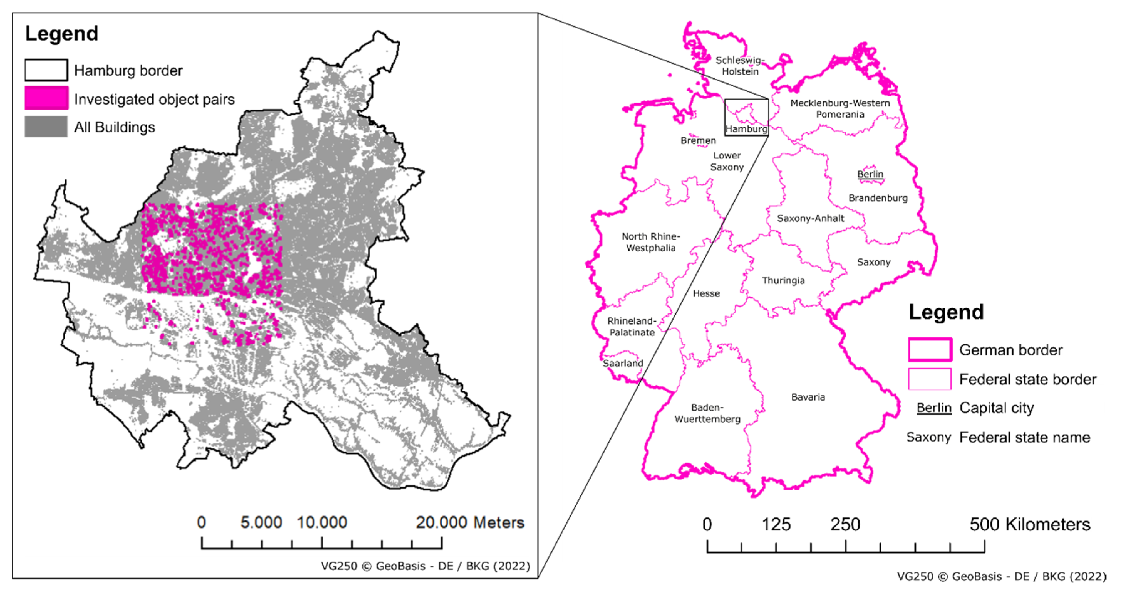
2.1. Case study and Input Data
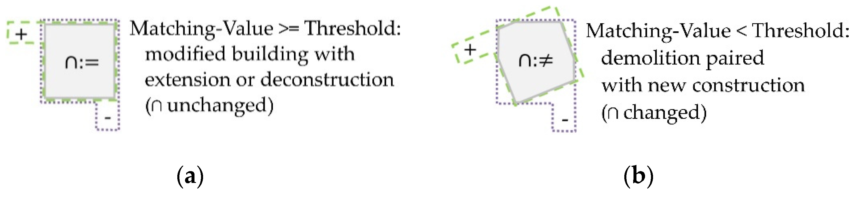
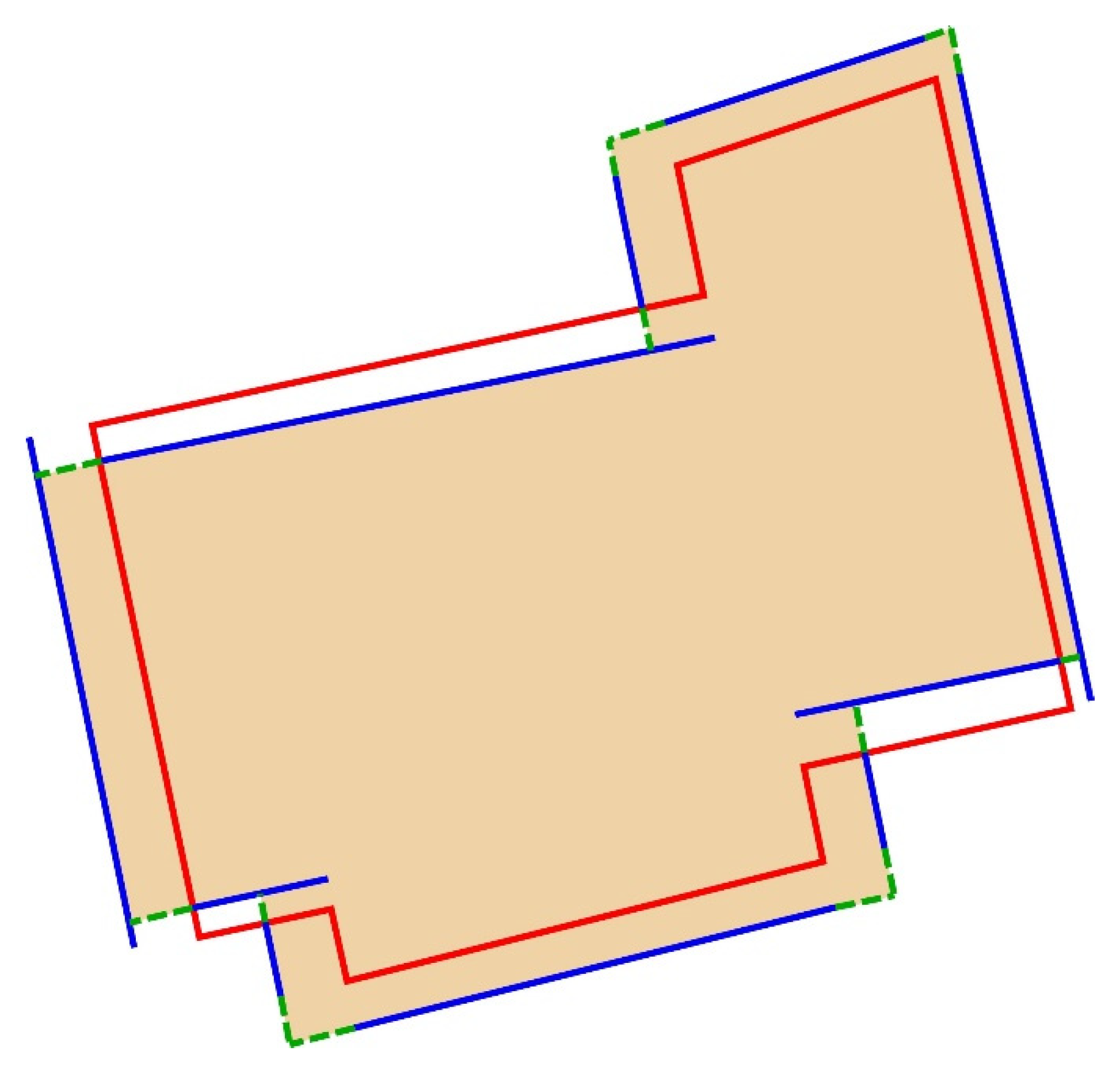
2.2. Types of Building Changes
2.3. Matching Procedures
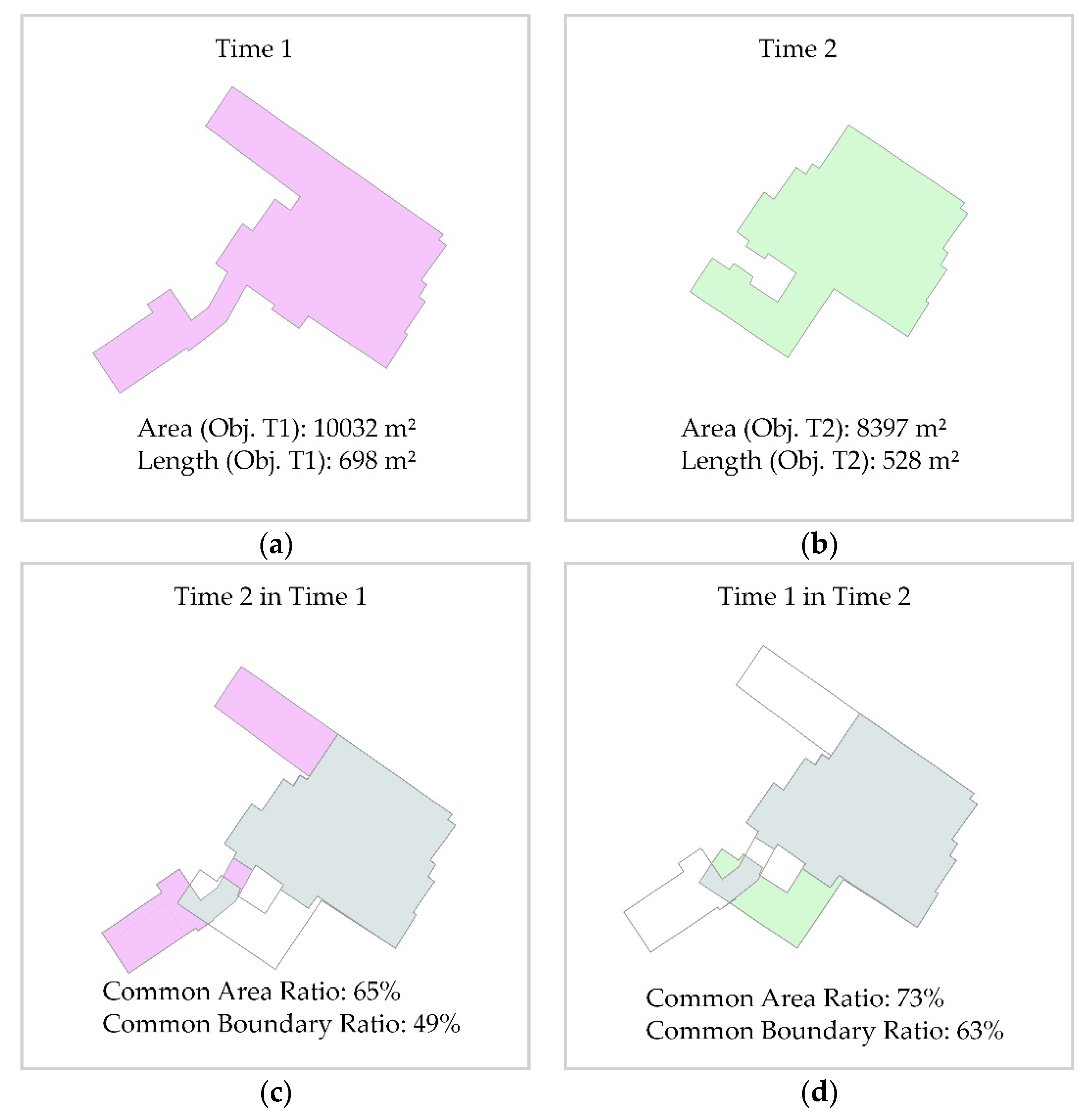
2.3.1. Common Area Ratio (CAR)
2.3.2. Common Boundary Ratio (CBR)
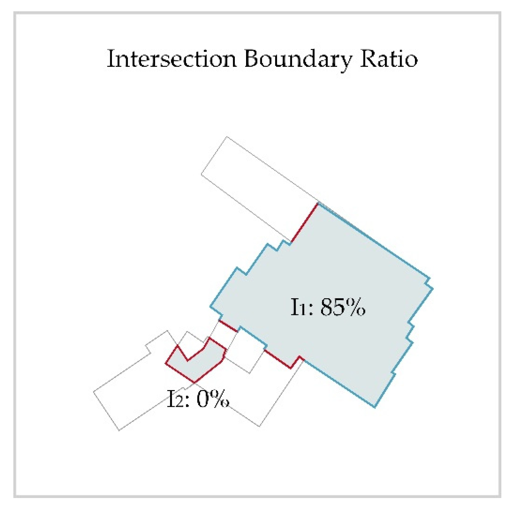
2.3.3. Intersection Boundary Ratio (IBR)
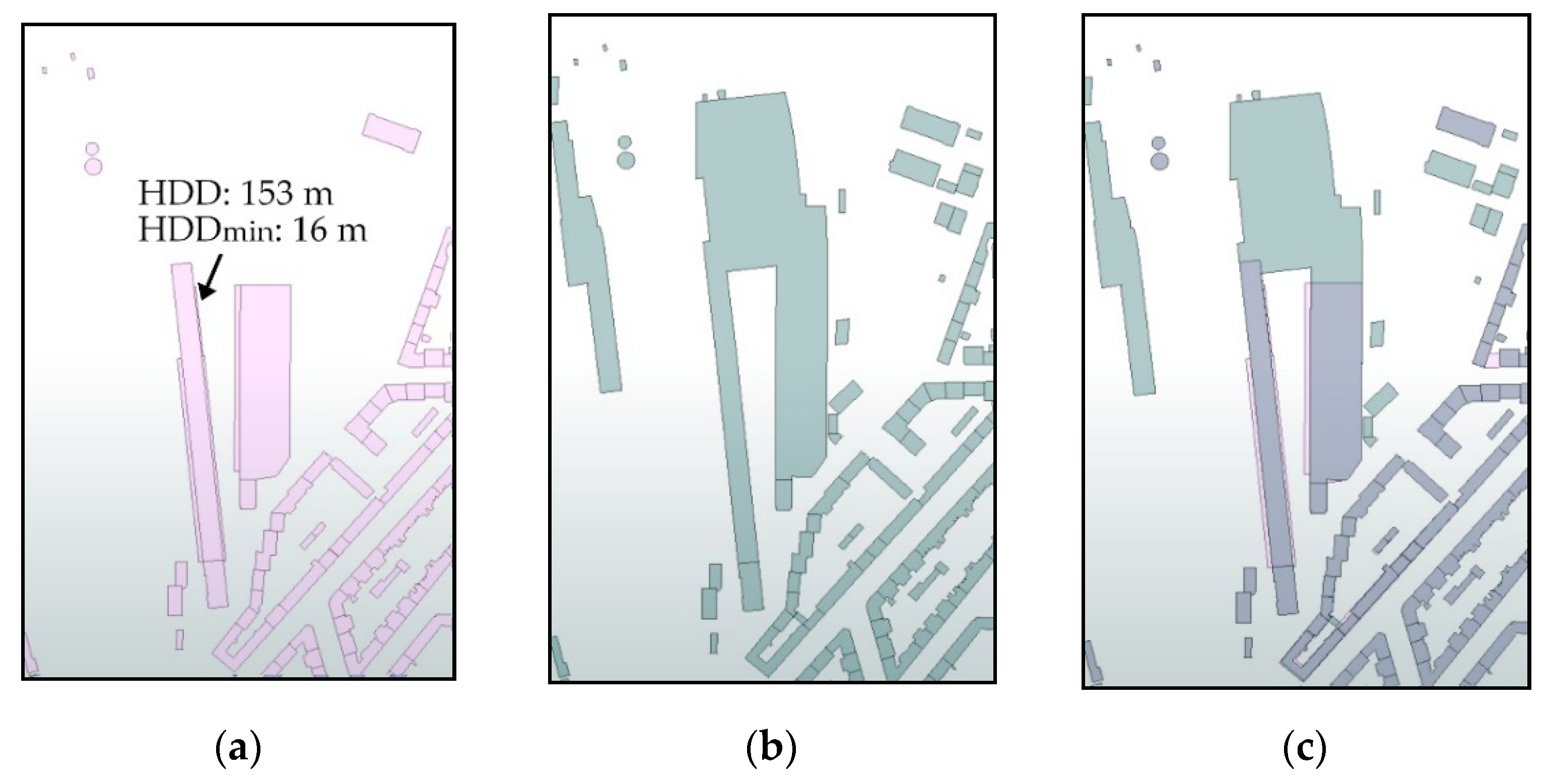
2.3.4. Hausdorff Distance (HDD)
2.3.5. Polygon and Line Segments (PoLiS)
2.4. Threshold and Error Determination
2.4.1. Optimal Threshold
2.4.2. Total Error
2.4.3. User Error
2.4.4. Producer Error
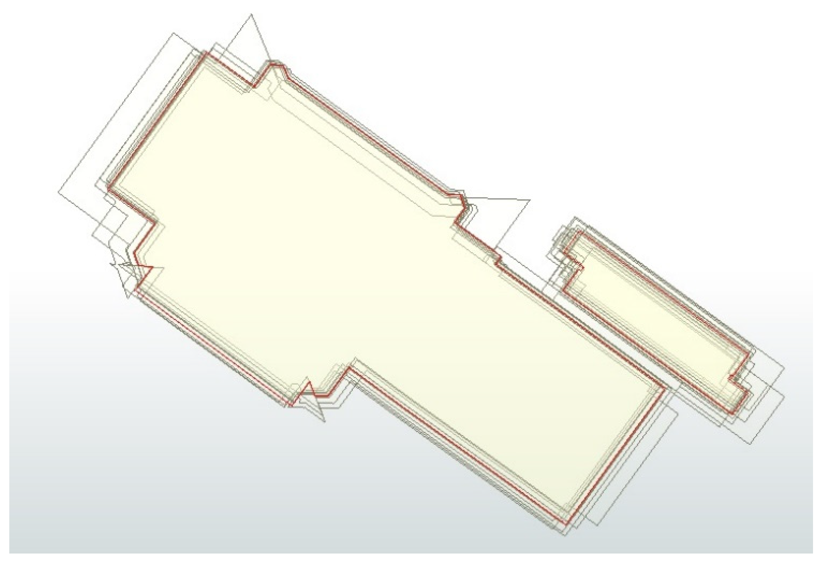
2.5. Generating Position Deviations
3. Results
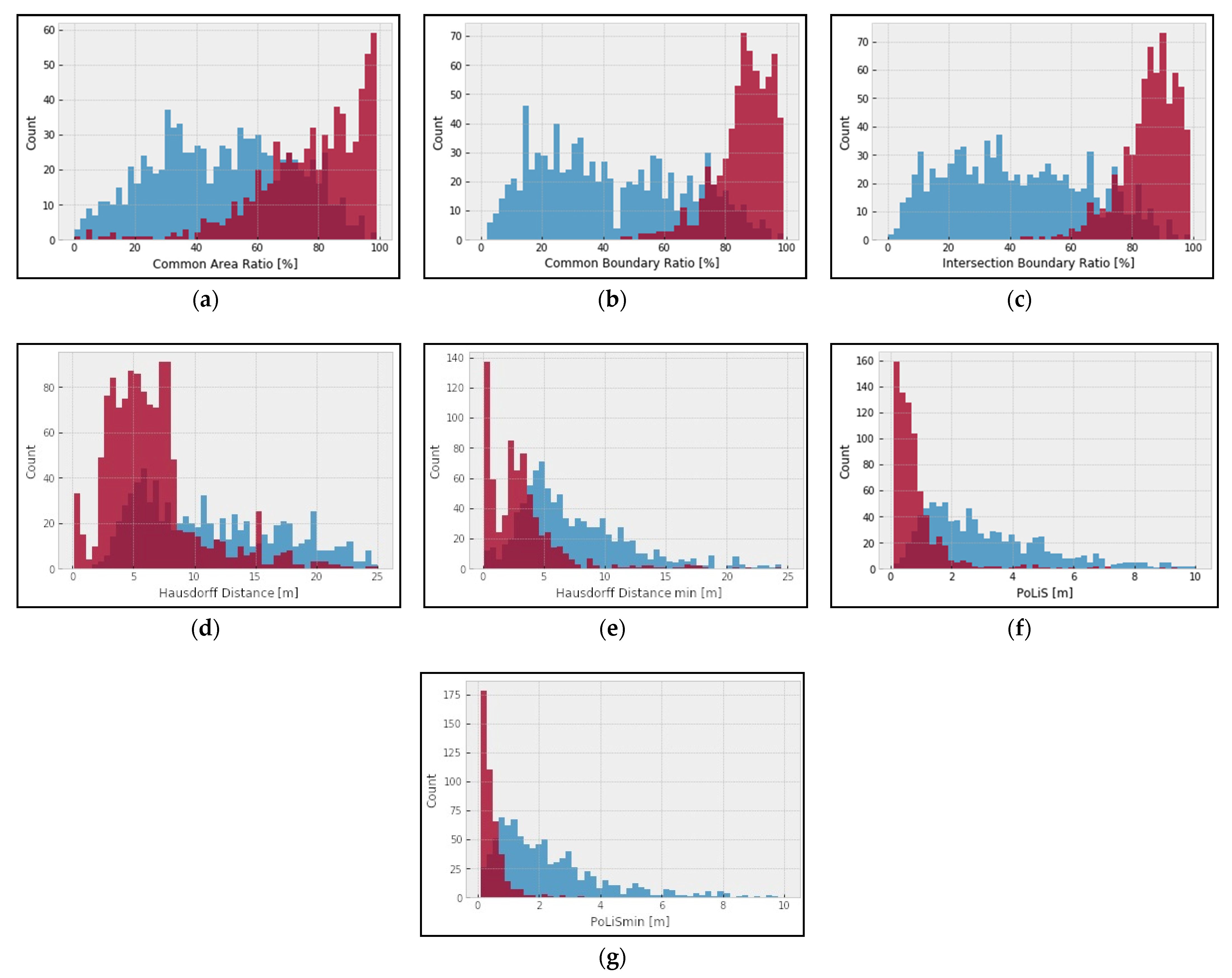
3.1. Distributions
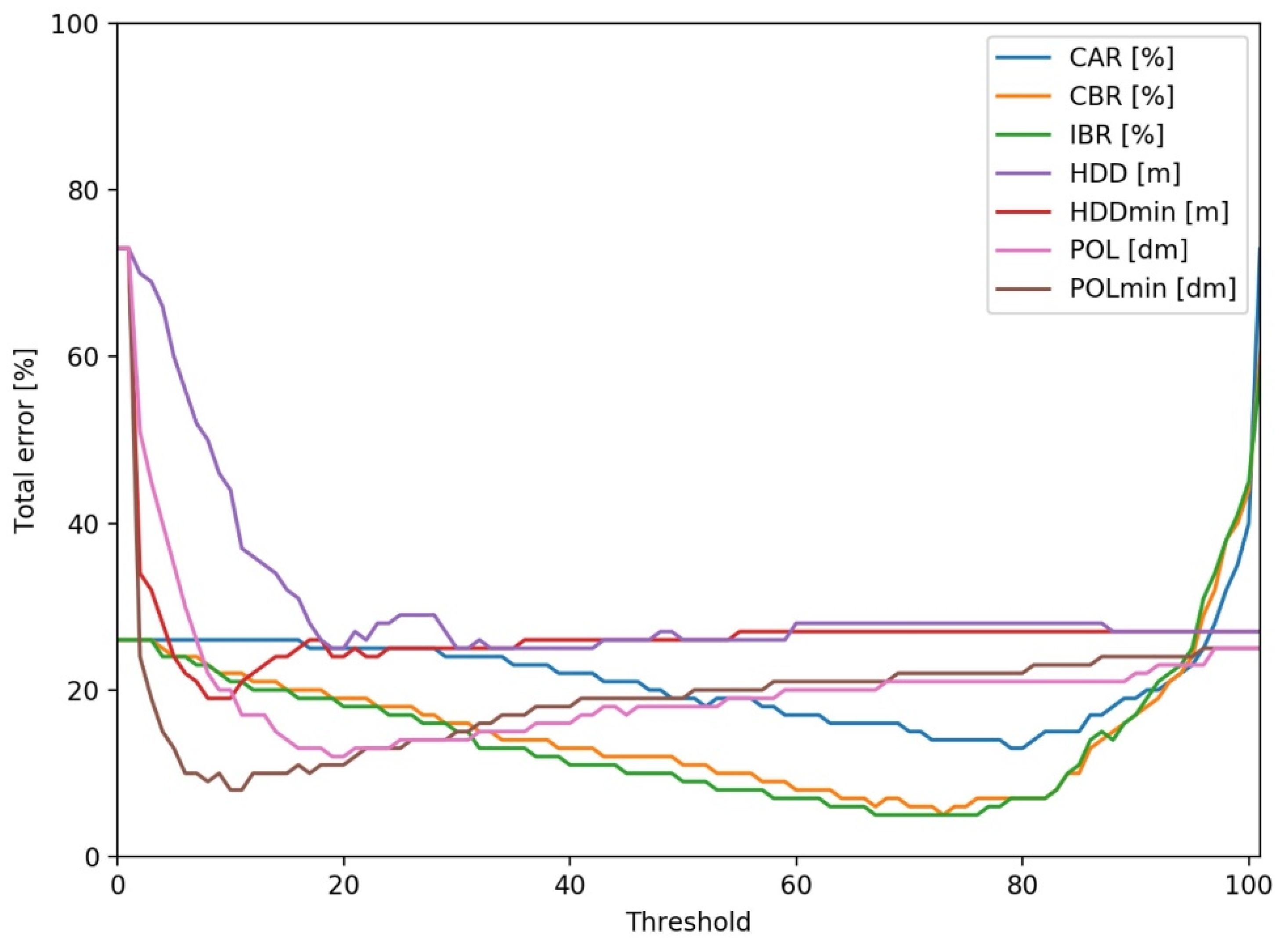
3.2. Optimal Thresholds and Accuracies
3.3. Thresholds and Accuracies of Generated Deviations
4. Discussion
5. Conclusions
Author Contributions
Funding
Institutional Review Board Statement
Informed Consent Statement
Data Availability Statement
Conflicts of Interest
References
- Biljecki, F.; Stoter, J.; Ledoux, H.; Zlatanova, S.; Çöltekin, A. Applications of 3D City Models: State of the Art Review. ISPRS Int. J. Geo-Inf. 2015, 4, 2842–2889. [Google Scholar] [CrossRef] [Green Version]
- Evans, S.; Liddiard, R.; Steadman, P. 3DStock: A New Kind of Three-Dimensional Model of the Building Stock of England and Wales, for Use in Energy Analysis. Environ. Plan. B Urban Anal. City Sci. 2017, 44, 227–255. [Google Scholar] [CrossRef] [Green Version]
- Vanderhaegen, S.; Canters, F. Mapping Urban Form and Function at City Block Level Using Spatial Metrics. Landsc. Urban Plan. 2017, 167, 399–409. [Google Scholar] [CrossRef]
- Biljecki, F.; Ohori, K.A.; Ledoux, H.; Peters, R.; Stoter, J. Population Estimation Using a 3D City Model: A Multi-Scale Country-Wide Study in the Netherlands. PLoS ONE 2016, 11, e0156808. [Google Scholar] [CrossRef]
- Broitman, D.; Koomen, E. The Attraction of Urban Cores: Densification in Dutch City Centres. Urban Stud. 2020, 57, 1920–1939. [Google Scholar] [CrossRef]
- Hecht, R.; Herold, H.; Behnisch, M.; Jehling, M. Mapping Long-Term Dynamics of Population and Dwellings Based on a Multi-Temporal Analysis of Urban Morphologies. ISPRS Int. J. Geo-Inf. 2019, 8, 2. [Google Scholar] [CrossRef] [Green Version]
- Khanal, N.; Uddin, K.; Matin, M.A.; Tenneson, K. Automatic Detection of Spatiotemporal Urban Expansion Patterns by Fusing OSM and Landsat Data in Kathmandu. Remote Sens. 2019, 11, 2296. [Google Scholar] [CrossRef] [Green Version]
- Ghamisi, P.; Rasti, B.; Yokoya, N.; Wang, Q.; Hofle, B.; Bruzzone, L.; Bovolo, F.; Chi, M.; Anders, K.; Gloaguen, R.; et al. Multisource and Multitemporal Data Fusion in Remote Sensing: A Comprehensive Review of the State of the Art. IEEE Geosci. Remote Sens. Mag. 2019, 7, 6–39. [Google Scholar] [CrossRef] [Green Version]
- Dai, C.; Zhang, Z.; Lin, D. An Object-Based Bidirectional Method for Integrated Building Extraction and Change Detection between Multimodal Point Clouds. Remote Sens. 2020, 12, 1680. [Google Scholar] [CrossRef]
- Sester, M.; Brenner, C. Datenquellen Und Methoden Für Eine Automatische Bestimmung von Gebäude- Und Siedlungsvolumen; Institute of Cartography and Geoinformatics—Leibniz University Hannover: Hannover, Germany, 2002. [Google Scholar]
- Matikainen, L.; Hyyppä, J.; Ahokas, E.; Markelin, L.; Kaartinen, H. Automatic Detection of Buildings and Changes in Buildings for Updating of Maps. Remote Sens. 2010, 2, 1217–1248. [Google Scholar] [CrossRef] [Green Version]
- Jabari, S.; Zhang, Y. Building Change Detection Using Multi-Sensor and Multi-View- Angle Imagery. IOP Conf. Ser. Earth Environ. Sci. 2016, 34, 012018. [Google Scholar] [CrossRef]
- Gergelova, M.B.; Labant, S.; Kuzevic, S.; Kuzevicova, Z.; Pavolova, H. Identification of Roof Surfaces from LiDAR Cloud Points by GIS Tools: A Case Study of Lučenec, Slovakia. Sustainability 2020, 12, 6847. [Google Scholar] [CrossRef]
- Avbelj, J.; Muller, R.; Bamler, R. A Metric for Polygon Comparison and Building Extraction Evaluation. IEEE Geosci. Remote Sens. Lett. 2015, 12, 170–174. [Google Scholar] [CrossRef] [Green Version]
- Fu, Z.; Fan, L.; Yu, Z.; Zhou, K. A Moment-Based Shape Similarity Measurement for Areal Entities in Geographical Vector Data. ISPRS Int. J. Geo-Inf. 2018, 7, 208. [Google Scholar] [CrossRef] [Green Version]
- Rottensteiner, F.; Sohn, G.; Gerke, M.; Wegner, J.D.; Breitkopf, U.; Jung, J. Results of the ISPRS Benchmark on Urban Object Detection and 3D Building Reconstruction. ISPRS J. Photogramm. Remote Sens. 2014, 93, 256–271. [Google Scholar] [CrossRef]
- Wu, J.; Wan, Y.; Chiang, Y.; Fu, Z.; Deng, M. A Matching Algorithm Based on Voronoi Diagram for Multi-Scale Polygonal Residential Areas. IEEE Access 2018, 6, 4904–4915. [Google Scholar] [CrossRef]
- Yang, M.; Ai, T.; Yan, X.; Chen, Y.; Zhang, X. A Map-Algebra-Based Method for Automatic Change Detection and Spatial Data Updating across Multiple Scales. Trans. GIS 2018, 22, 435–454. [Google Scholar] [CrossRef]
- Zhang, Y.; Huang, J.; Deng, M.; Chen, C.; Zhou, F.; Xie, S.; Fang, X. Automated Matching of Multi-Scale Building Data Based on Relaxation Labelling and Pattern Combinations. ISPRS Int. J. Geo-Inf. 2019, 8, 38. [Google Scholar] [CrossRef] [Green Version]
- Carleer, A.P.; Wolff, E. Change Detection for Updates of Vector Database through Region-Based Classification of VHR Satellite Data. In Remote Sensing for Environmental Monitoring, GIS Applications, and Geology VII; International Society for Optics and Photonics: Bellingham, WA, USA, 2007; Volume 6749. [Google Scholar]
- Qin, R. Change Detection on LOD 2 Building Models with Very High Resolution Spaceborne Stereo Imagery. ISPRS J. Photogramm. Remote Sens. 2014, 96, 179–192. [Google Scholar] [CrossRef]
- Abdessetar, M.; Zhong, Y. Buildings Change Detection Based on Shape Matching for Multi-Resolution Remote Sensing Imagery. ISPRS Int. Arch. Photogramm. Remote Sens. Spat. Inf. Sci. 2017, XLII-2/W7, 683–687. [Google Scholar] [CrossRef] [Green Version]
- Hartmann, A.; Meinel, G.; Behnisch, M.; Hecht, R. Gebäudebestandsmonitoring—Prozessierungsschritte für den Aufbau homogener Gebäudedatensätze. Flächensparen Ökosystemleistungen Handl. 2016, 69, 203–214. [Google Scholar]
- Meinel, G.; Krüger, T. Methodik eines Flächennutzungsmonitorings auf Grundlage des ATKIS-Basis-DLM. J. Cartogr. Geogr. Inf. 2014, 64, 324–331. [Google Scholar] [CrossRef]
- EEA. Urban Sprawl in Europe—Joint EEA-FOEN Report—European Environment Agency; Publications Office of the European Union: Luxembourg, 2016; Available online: https://data.europa.eu/doi/10.2800/143470 (accessed on 1 December 2021).
- DESTATIS. Qualitätsbericht—Flächenerhebung Nach Art der Tatsächlichen Nutzung; Statistisches Bundesamt (Destatis): Wiesbaden, Germany, 2018. [Google Scholar]
- Deutsche Bundesregierung. Die Deutsche Nachhaltigkeitsstrategie—Aktualisierung 2018; Presse-und Informationsamt der Bundesregierung: Berlin, Germany, 2018. [Google Scholar]
- Biljecki, F.; Ledoux, H.; Stoter, J. An Improved LOD Specification for 3D Building Models. Comput. Environ. Urban Syst. 2016, 59, 25–37. [Google Scholar] [CrossRef] [Green Version]
- Kaden, R.; Kolbe, T.H. City-Wide total energy demand estimation of buildings using semantic 3D city models and statistical data. In Proceedings of the ISPRS Annals of the Photogrammetry, Remote Sensing and Spatial Information Sciences, Istanbul, Turkey, 27–29 November 2013; Volume II-2-W1, pp. 163–171. [Google Scholar]
- Zhang, X.; Stoter, J.; Ai, T.; Kraak, M.-J.; Molenaar, M. Automated Evaluation of Building Alignments in Generalized Maps. Int. J. Geogr. Inf. Sci. 2013, 27, 1550–1571. [Google Scholar] [CrossRef]
- Brovelli, M.A.; Zamboni, G. A New Method for the Assessment of Spatial Accuracy and Completeness of OpenStreetMap Building Footprints. ISPRS Int. J. Geo-Inf. 2018, 7, 289. [Google Scholar] [CrossRef] [Green Version]
- Qin, R.; Tian, J.; Reinartz, P. 3D Change Detection—Approaches and Applications. ISPRS J. Photogramm. Remote Sens. 2016, 122, 41–56. [Google Scholar] [CrossRef] [Green Version]
- Fan, H.; Zipf, A.; Fu, Q.; Neis, P. Quality Assessment for Building Footprints Data on OpenStreetMap. Int. J. Geogr. Inf. Sci. 2014, 28, 700–719. [Google Scholar] [CrossRef]
- Pedrinis, F.; Morel, M.; Gesquière, G. Change Detection of Cities. In 3D Geoinformation Science; Lecture Notes in Geoinformation and Cartography; Springer: Cham, Switzerland, 2015. [Google Scholar] [CrossRef]
- Zhou, X.; Chen, Z.; Zhang, X.; Ai, T. Change Detection for Building Footprints with Different Levels of Detail Using Combined Shape and Pattern Analysis. ISPRS Int. J. Geo-Inf. 2018, 7, 406. [Google Scholar] [CrossRef] [Green Version]
- Schowengerdt, R.A. Remote Sensing: Models and Methods for Image Processing; Academic Press: Cambridge, MA, USA, 2006; ISBN 978-0-08-048058-9. [Google Scholar]
- Ghani, N.L.A.; Abidin, S.Z.Z. The Classification of Urban Growth Pattern Using Topological Relation Border Length Algorithm: An Experimental Study. In Recent Trends in Information and Communication Technology; Saeed, F., Gazem, N., Patnaik, S., Saed Balaid, A.S., Mohammed, F., Eds.; Springer International Publishing: Cham, Switzerland, 2018; pp. 545–553. [Google Scholar]
- Rutzinger, M.; Rottensteiner, F.; Pfeifer, N. A Comparison of Evaluation Techniques for Building Extraction From Airborne Laser Scanning. IEEE J. Sel. Top. Appl. Earth Obs. Remote Sens. 2009, 2, 11–20. [Google Scholar] [CrossRef]
- Veltkamp, R. Shape Matching: Similarity Measures and Algorithms. In Proceedings of the International Conference on Shape Modeling and Applications, Genova, Italy, 7–11 May 2001; pp. 188–197. [Google Scholar]
- AdV. Produktstandard für 3D-Gebäudemodelle Version 1.4; Arbeitsgemeinschaft der Vermessungsverwaltungen der Länder der Bundesrepublik Deutschland (AdV): Munich, Germany, 2017; p. 6. [Google Scholar]
- Cai, L.; Shi, W.; Miao, Z.; Hao, M. Accuracy Assessment Measures for Object Extraction from Remote Sensing Images. Remote Sens. 2018, 10, 303. [Google Scholar] [CrossRef] [Green Version]


| Title 1 | Time 1 | Time 2 | Time 1 ∩ Time 2 |
|---|---|---|---|
| New construction (Ø:n) | Ø |  |  |
| Demolition (n:Ø) |  | Ø |  |
| Replacement (demolition and new construction) |  |  |  |
| Modification (extension or deconstruction) |  |  | 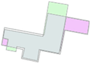 |
| Optimal Threshold | Total Area Error [%] | Replaced Area Error [%] | Modified Area Error [%] | |||
|---|---|---|---|---|---|---|
| User Error | Prod. Error | User Error | Prod. Error | |||
| CAR | 78% | 13.0 | 6.5 | 16.9 | 27.9 | 11.6 |
| CBR | 72% | 5.9 | 5.5 | 15.7 | 7.2 | 2.4 |
| IBR | 74% | 5.6 | 4.4 | 12.2 | 9.0 | 3.2 |
| HDD | 18.1 m | 25.3 | 14.9 | 38.4 | 47.9 | 20.6 |
| HDDmin | 6.9 m | 19.1 | 9.8 | 24.8 | 38.4 | 17.0 |
| PoLiS | 1.8 m | 12.7 | 7.5 | 20.1 | 25.7 | 10.0 |
| PoLiSmin | 0.9 m | 8.3 | 6.3 | 17.7 | 14.1 | 4.9 |
| Deviation Distance (m) | Optimal Threshold | ||||
|---|---|---|---|---|---|
| CAR (%) | CBR (%) | IBR (%) | HDDmin (m) | PoLiSmin (m) | |
| 0.25 | 78.6 | 73.6 | 72.3 | 7.4 | 1.10 |
| 0.50 | 78.6 | 77.9 | 73.2 | 7.7 | 1.28 |
| 0.75 | 77.1 | 77.8 | 72.7 | 8.9 | 1.47 |
| 1.00 | 74.2 | 78.0 | 73.1 | 8.9 | 1.63 |
| 1.25 | 72.9 | 77.2 | 74.5 | 8.3 | 1.55 |
| 1.50 | 70.4 | 76.4 | 73.0 | 7.9 | 1.89 |
| 1.75 | 70.0 | 74.4 | 73.0 | 7.8 | 2.09 |
| 2.00 | 65.5 | 81.0 | 75.3 | 8.0 | 2.32 |
| 2.25 | 62.1 | 79.6 | 75.2 | 7.6 | 2.46 |
| 2.50 | 59.9 | 78.2 | 75.7 | 7.7 | 2.60 |
| 2.75 | 59.0 | 77.3 | 76.2 | 8.3 | 2.77 |
| 3.00 | 59.5 | 78.4 | 77.7 | 8.3 | 3.05 |
| 3.25 | 58.7 | 77.6 | 75.3 | 8.9 | 3.17 |
| 3.50 | 55.2 | 78.8 | 77.5 | 10.2 | 3.30 |
| 3.75 | 57.3 | 76.6 | 74.0 | 8.3 | 3.43 |
| 4.00 | 52.7 | 79.0 | 79.0 | 9.0 | 3.60 |
| 4.25 | 51.1 | 76.5 | 76.3 | 8.9 | 3.77 |
| 4.50 | 52.9 | 78.1 | 75.8 | 10.3 | 4.09 |
| 4.75 | 48.8 | 78.6 | 75.2 | 11.9 | 4.31 |
| 5.00 | 46.8 | 81.3 | 77.6 | 11.1 | 4.25 |
Publisher’s Note: MDPI stays neutral with regard to jurisdictional claims in published maps and institutional affiliations. |
© 2022 by the authors. Licensee MDPI, Basel, Switzerland. This article is an open access article distributed under the terms and conditions of the Creative Commons Attribution (CC BY) license (https://creativecommons.org/licenses/by/4.0/).
Share and Cite
Schorcht, M.; Hecht, R.; Meinel, G. Comparative Study on Matching Methods for the Distinction of Building Modifications and Replacements Based on Multi-Temporal Building Footprint Data. ISPRS Int. J. Geo-Inf. 2022, 11, 91. https://doi.org/10.3390/ijgi11020091
Schorcht M, Hecht R, Meinel G. Comparative Study on Matching Methods for the Distinction of Building Modifications and Replacements Based on Multi-Temporal Building Footprint Data. ISPRS International Journal of Geo-Information. 2022; 11(2):91. https://doi.org/10.3390/ijgi11020091
Chicago/Turabian StyleSchorcht, Martin, Robert Hecht, and Gotthard Meinel. 2022. "Comparative Study on Matching Methods for the Distinction of Building Modifications and Replacements Based on Multi-Temporal Building Footprint Data" ISPRS International Journal of Geo-Information 11, no. 2: 91. https://doi.org/10.3390/ijgi11020091
APA StyleSchorcht, M., Hecht, R., & Meinel, G. (2022). Comparative Study on Matching Methods for the Distinction of Building Modifications and Replacements Based on Multi-Temporal Building Footprint Data. ISPRS International Journal of Geo-Information, 11(2), 91. https://doi.org/10.3390/ijgi11020091