Abstract
Agent-based modeling has the potential to deal with the ever-growing complexity of transport systems, including future disrupting mobility technologies and services, such as automated driving, Mobility as a Service, and micromobility. Although different software dedicated to the simulation of disaggregate travel demand have emerged, the amount of needed input data, in particular the characteristics of a synthetic population, is large and not commonly available, due to legit privacy concerns. In this paper, a methodology to spatially assign a synthetic population by exploiting only publicly available aggregate data is proposed, providing a systematic approach for an efficient treatment of the data needed for activity-based demand generation. The assignment of workplaces exploits aggregate statistics for economic activities and land use classifications to properly frame origins and destination dynamics. The methodology is validated in a case study for the city of Tallinn, Estonia, and the results show that, even with very limited data, the assignment produces reliable results up to a 500 × 500 m resolution, with an error at district level generally around 5%. Both the tools needed for spatial assignment and the resulting dataset are available as open source, so that they may be exploited by fellow researchers.
1. Introduction
1.1. Context and Motivation
In urban areas in the United States alone, in 2017, congestion resulted in 8.8 billion extra hours of travel time, an extra 3.3 billion gallons of purchased fuel, and an overall cost of USD 166 billion [1]. A similar picture appears in Europe, with a congestion cost estimated at approximately EUR 110 billion per year, in terms of delay [2], while urban mobility accounts for 40% of all CO2 emissions from road transport [3]. This is expected to become more complex in the following decades, with trends such as urbanization common to most of the globe [4]. An increased population entails issues, such as urban sprawling, further load on transport networks, and increased levels of emissions. Different smart mobility solutions to these problems are being developed and tested in urban areas, with the concept of smart cities becoming more common [5]. Still, new solutions often require new assessment tools and smart mobility solutions are no exception. The higher flexibility enabled by digitalization requires that a certain level of disaggregation be captured by assessment models and tools, which cannot be framed by the traditional macroscopic transport models, i.e., models that consider aggregate people/vehicle flows. This prompted a surge of activity-based and agent-based models (ABMs) resulting in an increase of data reliance and complexity, which is hindering their uptake and slowing down research [6]. Other hindering factors are, for example, the lack of dedicated skillsets and tools to handle increased data processing complexity or higher computational demands.
Through ABMs, it is possible to simulate mobility decisions down to the individual (agent) level. This allows modeling and forecasting travel behavior that is sensitive to socioeconomic features and individual characteristics, to a level that is not achievable using the traditional four-step models. Moreover, the agents make travel demand choices based on the transport supply performance, which allows, for example, to implicitly generate induced demand [7]. These features were relevant already before the COVID-19 crisis and it is fair to assume that the pandemic will speed up changes in mobility behavior. Moreover, more flexible and complex mobility solutions are being developed or already deployed in cities across the globe, such as, e.g., automated vehicles, Mobility as a Service (MaaS) applications, and micromobility solutions. The effects of each one, as well as of combinations of them, on transport demand is not yet univocally framed, which in turn makes aggregate models sub-optimal for assessment and future predictions.
Significant limits of ABMs surround how data reliant they are and how complex their settings are. The population of agents in an ABM includes all the residents in the study area and details some relevant characteristics of each individual, such as household structure, age, gender, employment status, etc. This kind of dataset is almost never available due to more than legit privacy concerns (https://www.fsd.tuni.fi/en/services/data-management-guidelines/anonymisation-and-identifiers/; accessed on 28 December 2021) and should be built from mobility surveys and relevant statistics. While tools to build these datasets already exist and will be reviewed in the following paragraphs, usually the output does not yet reach the degree of precision required by most advanced ABMs and, when it does, it is thanks to the exploitation of additional methodologies and seldom available data sources.
This paper aims at filling a gap in literature concerning the assignment of a synthetic population to a grid of arbitrary dimensions, namely, to a resolution of choice, by exploiting only publicly available data. This is achieved by a novel methodology for the synthetic population assignment that exploits land use data and NACE (https://ec.europa.eu/competition/mergers/cases/index/nace_all.html accessed on 28 December 2021) margins to keep consistency in residence–workplace patterns. The result is a systematic approach, i.e., which does not leave any passage undetailed, is highly replicable, and designed to be flexible and nimble. In particular, the level of disaggregation can be freely designed, while the code implementing this methodology is provided as open source and customizable as needed.
In this paper, we provide an overview of the state of the art concerning the generation and assignment of a synthetic population. We highlight how the available methods and tools do not necessarily produce results at a desirable spatial disaggregation level, while employing publicly available data. Thus, the authors argue, this calls for a method that exploits public data to carry out the spatial assignment linking synthetic populations with ABMs.
1.2. Literature Review
ABMs need a dataset representing the population living, working, studying, and travelling within the modeled area. Various methods and tools have been proposed to build a statistically representative synthetic version of the real population. One tool is the iterative proportional updating (IPU) procedure described in [8]. IPU processes a sample of disaggregate individuals and aggregate distributions of relevant features at certain geographical resolutions; as an example, the case study in [8] produced a population of 4.5 million individuals for the Great Munich area. However, as in most cases, not all variables were available as inputs and variables, such as workplaces or residences were allocated through Monte Carlo sampling; still, this process is not detailed in the paper. The work in [9] synthesizes individuals and households with a fitness based synthesis algorithm instead, building a case study in Atlantic Canada. The input data were the Canadian Census and the Canadian Census hierarchical public use microdata file. The obtained synthetic population is characterized by the following variables: gender, age, ethnicity, immigrant, citizenship, household size, tenure, dwelling type, and household income. Still, these variables are too few to satisfy ABM requirements, since relevant ones, such as residence, workplaces, but also employment sector and/or status, are missing. Another tool to generate synthetic populations from travel diaries and census margins is SimPop [10], which allows approaches such as model-based generation and calibration through simulated annealing. Moreover, SimPop can be utilized for very large-scale scenarios, even at country level; in [10] it is shown to generate synthetic population of the whole Austria. Still, no anchor point, i.e., a key place in the life and schedule of an individual, is produced when it comes to workplaces or education.
Information about spatial patterns of housing is considered in [11], where a two level iterative proportional fitting (IPF) method is applied, assigning residents to each building while exploiting data such as dwelling type and household income. As detailed above, this degree of precision is actually rare in literature; however, this comes at the cost of utilizing data that is rarely available, such as the average transaction prices or building capacities. Moreover, in this case, the degree of precision may be unnecessarily high for ABM setting in the context of transport demand modeling. Finally, existing literature suggests that IPU outperforms IPF in terms of generation of a population, since the latter does not allow matching the joint distribution both at the individual and at the household level at the same time [10]. Besides, further improvements of the IPU algorithm have been proposed in time. In [12], for example, the IPU algorithm is updated to be able to control for constraints at multiple geographic resolutions when generating a synthetic population. A wide portion of the literature focuses on generation of synthetic populations: a review of related tools and methods is provided in [13]. In the following, only works focusing on the assignment of anchor points (e.g., school or workplaces) will be further analyzed.
In [14], two synthetic generation methods (one sample-based and one non-sample-based) are tested on a portion of the French population; however, the focus of the paper is the comparison between the methodologies and few details about the input and the achievable output data are provided, while no ex-post spatial assignment is performed. The work in [15] adds land use variables in the generation of synthetic population and the results suggest that the addition of such variables improves the capability to frame additional nuances, such as, e.g., the differences in mobility patterns between rural and urban areas. In [16], the assignment of schools and workplaces is performed based on different assumptions to tackle the lack of data related to enrolling and commuting patterns. While for education, age and distances were the main factor defining enrollment, the workplaces were assigned randomly within counties (still in a way to meet total margins from the census).
A different approach for the population assignment is suggested in [17], where a synthetic population of establishments (i.e., places of business) is built first for an ABM model (the SimMobility platform). The authors then suggest that such results may be exploited to assign anchor points to the population, since all of the relevant information are modeled. Still, some of the required data are rarely available, such as, e.g., the establishment locations, industry type, employment size, and occupied floor area. Paper [18] reports exploiting floor areas as well, together with public transport smart card data.
In [19], different prototype cities, populations, and mobility patterns are built to create different scenarios; in particular, the prototype population is constructed by assigning spatial features based on land use characteristics. However, the paper neither explores patterns between residence and workplace location, nor details how a model is applied to fill this gap (note that a gravity model accounts for some estimates of origins and destinations between zones and then relates them through a distance factor, considered as impedance, to generate an amount of trips. Further details may be found in [20]). It is then left unclear how the solution actually reproduces commuting patterns; moreover, since the assignment of the synthetic population is not at the core of [19], their methodology is not detailed. Another work that applies a gravity model to assign workplaces is [21], but the focus outside of the transport domain led to a simplistic approach, in which only distance and capacity were considered. Besides, in this study, capacity of the establishments was not available as spatial data. Still, the approach in [21] is interesting since it attempts to tackle the lack of dedicated open-source software with an open-source application coded in R, which is a feature that this paper also implements, albeit with a narrower focus. Similarly, [22] only considers the size of the company and distance for the assignment. In [23], a connection between jobs and individual features, such as educational level or gender, is modeled. Still, from [23] itself, it is not clear if the above was exploited in what is described as an empirical gravity model. Paper [24] goes one step further in this direction and develops a utility-based model tying personal characteristics of the individual to the workplace location (including the choice of working from home as well). Still, this was made possible by the availability of a reliable household activity survey and state unemployment insurance records detailing the locations of employment. The approach in [23,24] goes in the same direction as the NACE assignment implemented in this paper. On the other hand, the level of spatial disaggregation reached in this study (500 × 500 m) is much lower than in [23,24] due to different study area’s scales.
Another recent study tackling the workplace assignment issue for synthetic populations is [25], in which an origin–destination industry matrix is exploited to assign workplace probabilities to the synthetic population for the Greater Boston Area. While this approach allows exploiting observed patterns rather than assuming theoretical models, such origin-destination industry matrices are rarely available. Similarly, reference [26] exploits data, such as commuting patterns, commuting OD matrices and distance travelled to carry out the assignment of workplaces for a synthetic population through multinomial distribution. Paper [27], instead, employs records about business and related employees counts, in addition to residence-workplace distributions between census tracts. However, the spatial scale of [27] is not comparable to the one of this study since it focuses on the whole US population. This in turn entails bigger analysis zones, which explains the availability of the residence–workplace distribution. A slightly different approach is taken in [28], where the job-housing balance is assessed through a utility-based method. While the work assesses different scenarios in which residences and workplaces are chosen in Beijing, the focus is on finding the optimal job-housing distribution rather than framing the real disaggregate workplace distribution.
A good overview of the current state of the art is given in [29], which expands the state of the art by building both a synthetic population and the arising travel demand with only open and publicly available data. The developed pipeline was also tested in [30]. The work in [29] makes a good case about why research in this area is needed, namely how other current approaches are rarely systematically tested and hardly transferable. While the aim and contribution are similar, some challenges are addressed in the presented paper that are not addressed in said work. For example, in [29], data concerning the commuting matrices were openly available and could be used as proxies. This is not the case in other locations (including Estonia), where other statistical information (e.g., the NACE margins) should be exploited instead. Moreover, information related to businesses has a high level of detail in [29], while in this paper again statistical information and land use data are exploited as proxies to assign workplaces. Finally, the household travel surveys exploited in [29,30] had enough entries to allow correlations between socioeconomic features and commuting distances/anchors (consequently, it facilitates to build the daily activity schedules for the synthetic population). This was not the case in our work. Therefore, the method reported in this paper differs from [29], bypassing the need for an OD matrix and reliable entries in the household survey, even though both the motivation of the work and the aims are similar. Both works attempt to provide a runnable pipeline simple and as reproducible as possible, built only on publicly available data. To the knowledge of the authors, aside [29] and the presented paper, no other work investigates similar methods or challenges the state of the art in a similar way.
To summarize, in the literature, the small but crucial step of assigning a synthetic population to disaggregated spatial units seems either to rely on very detailed data, e.g., about firms and commuting patterns, or to be limited to aggregate margins and probability distributions. One of the many ABM examples of the latter is in [31], a work exploiting MATSim. The paper reports how residence and workplace locations were randomly assigned in areas with coherent land use (e.g., no residence is assigned to land use zones without residential buildings). Indeed, [31] is very relevant as an example because it explicitly aims to use only publicly available data to build the model. Still, this solution is not feasible in cases where only very aggregate data are available (i.e., in the case study presented below, where workers totals were available only at district level).
Finally, even though some tools have embedded functions or plugins to assign anchor points (e.g., ct-ramp (https://www.ct-ramp.com/ accessed on 28 December 2021)), others do not (e.g., SimMobility MT (https://github.com/smart-fm/simmobility-prod/wiki/Introduction-to-SimMobility accessed on 28 December 2021)) and the latter need agile methods to implement this assignment. The proposed methodology is independent from any ABM software and can be used regardless of the model that is being exploited. The methodology presented in this paper is conceived to be both less reliant on firms’ data/ commuting OD matrices and nimble enough to integrate additional inputs. Besides, it is the only solution, to the authors’ knowledge, that makes up for the lack of disaggregated statistics with the introduction of NACE fields.
What Table 1 tries to intuitively show is that no other study present in the literature aims at carrying out the workplace assignment with as minimal data as the proposed one. It should appear clearer then how providing a systematic approach to tackle the challenge of assigning anchor points to a synthetic population, employing only public data, may allow the state-of-the-art to further move forward ABM. By exploring the literature, it is evident that no approach allows researchers to fit synthetic populations for ABM in a formalized, efficient, and quick way while exploiting a minimal set of publicly available data, aggregate margins, and land-use features, regardless of the exploited tools. That is the research gap this paper tries to fill.

Table 1.
Comparison in data requirements between the presented paper (PP) and the other relevant studies from literature. In the table, random assignment was added to take into account a key limitation related to sparse datasets. The NACE row is highlighted as well to remark how the presented method is the only one exploiting this data source, to the best of our knowledge.
1.3. Paper Structure
The paper is structured as follows. In Section 2, the proposed methodology is described and detailed, In Section 3, a case study implemented for the city of Tallinn, Estonia, is introduced, while describing how the proposed method is implemented. In Section 4, the resulting dataset is presented and validated against the available statistical distributions. Section 5 contains a discussion on how the obtained results fill the gap identified in the introduction, while future research directions are also highlighted. Finally, in Section 6, a short summary of the presented work is provided and conclusions are stated.
2. Materials and Methods
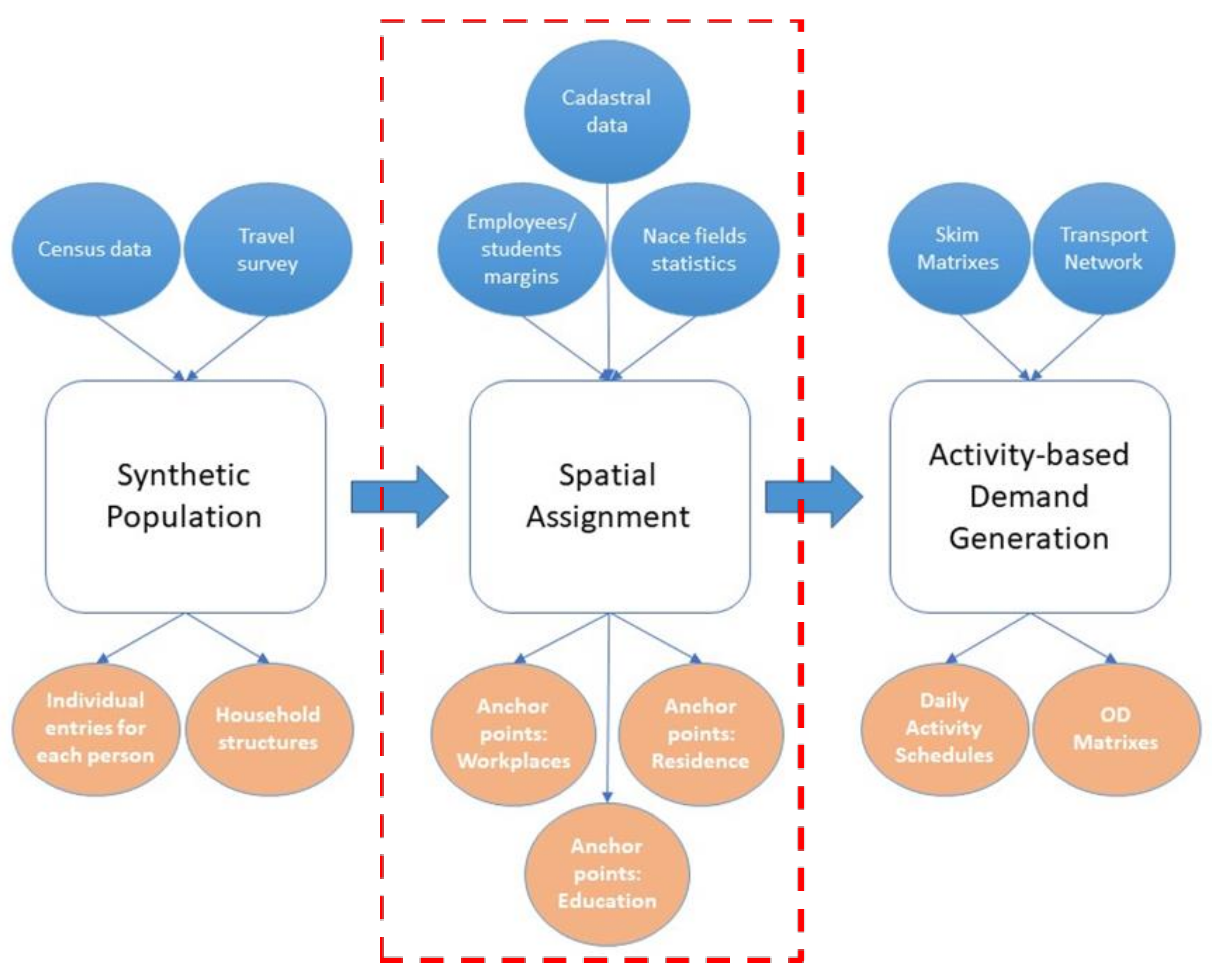
As previously argued, the generation of a synthetic population does not frame all of the anchor points needed to design an activity based model. Indeed, an intermediate step is needed: the spatial assignment of the population to a level of disaggregation that is fit for the required implementation. Input of this step are the generated synthetic population and, for the proposed methodology, statistical data, such as cadastral data, industry statistics, and total employees’ or students’ margins, as reported in Figure 1. The output of this step is the synthetic population integrated with anchor points, input for activity-based demand generation. The outputs have been widely tested on SimMobility, Preday, but should fit any activity-based demand generation model.
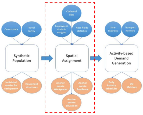
Figure 1.
Conceptual framework: from generating the synthetic population to activity-based modeling.
The novel contribution of this paper focuses essentially on the highlighted part in Figure 1, namely the spatial assignment of anchor points, while assuming other state-of-the-art methods are employed for the other components.
Before presenting the proposed methodology, we briefly summarize the most relevant method existing in literature [19], which was developed for building different prototype cities with their prototype population, where spatial features are assigned based on land use characteristics and distance. The algorithm proposed in [19] can be summarized as follows.
First, weights for different cell classes are defined as:
where is the weight of class X = {L,H,C,I,E,O}, defined as: low residential (L), highly residential (H), commercial (C), industrial (I), education (E), and open land (O). Cells may be defined based on the case study at hand and reflect different distributions of cadastral patterns. If the dimension of the cells varies greatly it would be recommended to add the occupied area in the computation of the cell weight. The following formulation was instead conceived for cells of equal dimensions (regardless of the actual dimension). Then, the cell weights are normalized within each subzone (i.e., second administrative district level), according to:
where i indexes cells, s indexes subzones, and is the set of cells within subzone s. By weighting the cells against the total in each subzone, the method becomes applicable to any number and type of cadastral classes. The number of workplaces in each cell within a subzone, , is then computed by multiplying the normalized weight by the total number of workers within a subzone :
Finally, distance is used for a last mile assignment of the workplaces to the population. This method allows performing the synthetic population assignment relying on data that are commonly publicly available, such as land use data. The degree of disaggregation that is reached is indeed sufficient to build accurate activity-based models, since the dimension of the cells can be arbitrarily defined. However, this method does not explore how a final gravity model-based assignment is carried out for the workplace, nor if any kind of further spatial consistency or commuter patterns across subzones are considered in the workflow. Therefore, it is not clear how closely the residence–workplace relationship is matched through the presented method. By including the NACE assignment, our work tries to build on such framework to include factors other than land use and distance. Moreover, describing the gravity assignment and the results should foster transferability and replicability of the proposed methodology.
2.1. Assignment of NACE Fields to the Population
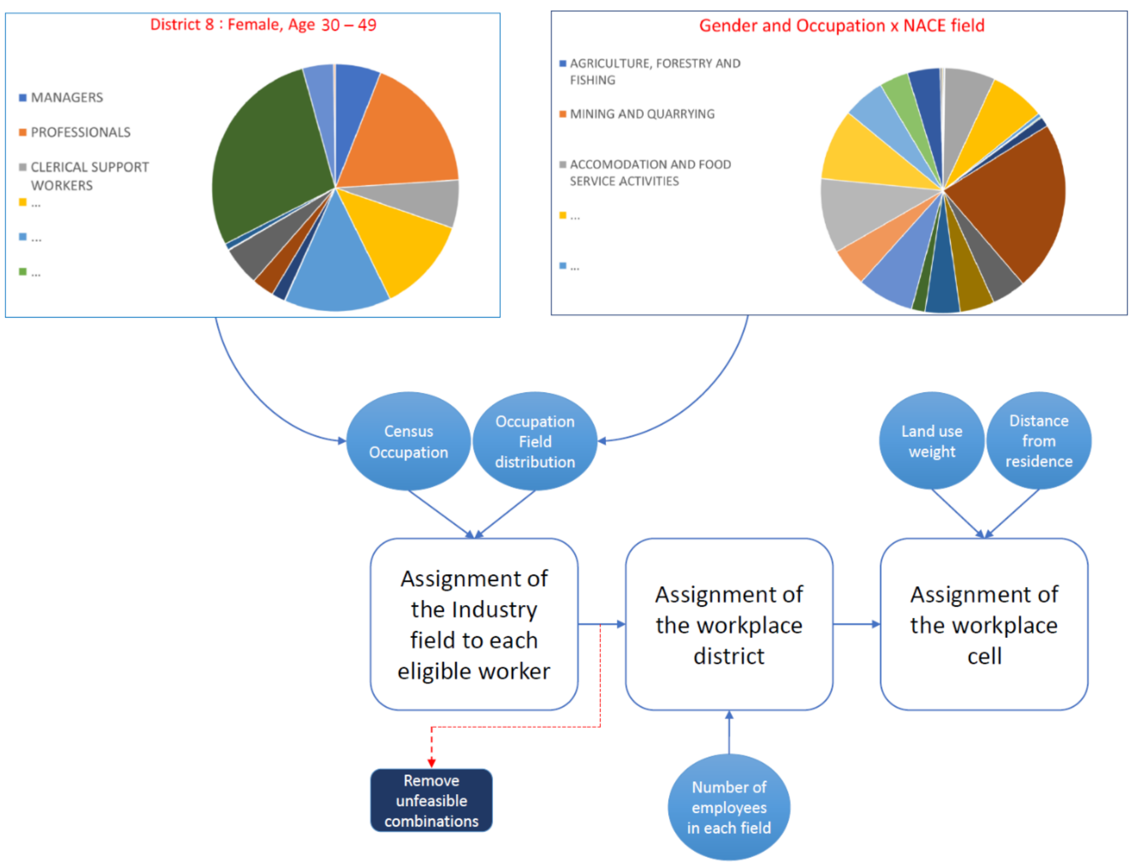
The first proposed step consists in exploiting census data to obtain the distribution of workers by their occupation status and their NACE classes (or their NAICS (https://www.census.gov/naics/ accessed on 28 December 2021) ones, or similar), based on gender, age, and district of residence (as recorded from the national census—the EMTAK classification, national version of the NACE classification, was exploited). The assignment is implemented through probability distributions such as occupation per age, gender, and district of residence. At the end of the assignment, unfeasible or very unlikely combinations, such as, e.g., 20 years old managers, should be removed, by reassigning the occupation status. This process is illustrated in Figure 2.

Figure 2.
Workplace assignment—phases and example of data exploited.
Once the assignment of the NACE (or equivalent) field is performed, the amount within the synthetic population is checked against the total number of employees within the city, as recorded for example by the business census. Indeed, we should consider that the synthetic population, while representative of the overall population, may misrepresent some distributions depending on the distributions it is calibrated against [10]. This may lead to skewed totals in some NACE fields or in some districts/subzones. Moreover, it may happen that the NACE dataset and the business register are not consistent with each other.
2.2. Subzone Assignment
In case no inconsistencies between datasets are detected, the district containing the workplace for each individual is assigned so that the totals per NACE field are met. The assignment is carried out extracting random samples based on the probability distribution NACE field per district of work. The NACE field is assigned based on age, gender, and residence through the occupation distribution. A stronger tie between these variables and the working district is therefore achieved compared to the one that would have been obtained by simply exploiting aggregates to derive a distribution while matching the total employees’ margins. In the following, Algorithm 1 summarizes this first phase. List of probabilities1 represents the distribution of occupations as per census margins while list of probabilities2 bridges occupations with NACE fields. In the latter, all NACE fields that are inconsistent are clustered under “Other”. The R sample function (https://www.rdocumentation.org/packages/base/versions/3.6.2/topics/sample accessed on 28 December 2021) is exploited to apply different distributions based on age (A), gender (G), district of residence (DoR) and student status (S); * values represent various combinations of individual features, related to different distributions.
| Algorithm 1 NACE assignment (individual, occupation distribution {A, G, DoR, S}, NACE distribution {G, O}) |
| 1: Loop: Individuali <- Population |
| 2: If ({Ai, Gi, DoRi, Si} == {A, G, DoR, S} and Occupation == NA |
| 3: Occupation<-sample(list of occupations, size = 1, list of probabilities1) |
| 4: NACE<-sample(list of NACE fields, size = 1, list of probabilities2) |
| 5: Else |
| 6: NACE assignment (Individual, occupation distribution {A*, G*, DoR*, S*}, |
| 7: NACE distribution {G*, O*} |
For the “Other” cluster, we first compute the distance between each residence cell and each other subzone (); then the first subzone gravitational pull, namely the number of employees not already assigned to another NACE field, is considered and the probability for each individual to work in one of the districts is computed as:
where j is the district of work, is the number of employees in said district, and i is the cell of residence.
Despite this method may add some noise to the total number of jobs in a district, spatial integrity is preserved, i.e., people from one side of the city are less likely to work on the other side of the city. However, this step is needed to keep this assignment comparable to the one for coherent NACE fields. Moreover, as it will be showed in the case study, the number of employees assigned this way in each subzone remains fairly consistent with the real-world data. It is worth highlighting here how the presented work tries to build on [19] and what are the differences. The main one is the NACE assignment step, summarized in Figure 2 and in the reported algorithm; by building a residence–workplace correlation, the relevance of the distance factor is strongly reduced and different dynamics may be framed; for example, the share of workers with very long commutes is arguably better framed this way, since their overall margin is defined. In [19], instead, longer paths seem to be strongly penalized. This changes how the following steps are implemented (e.g., Equation (5) assigns a class before computing the probability of working in a certain cell).
Another key difference lies in [19] not reporting the results of the various steps and only describing the pipeline in the appendix(the focus of said work is not the spatial assignment). Therefore, the replicability of the method is hindered and the degree of reliability of the results is never assessed. By reporting each passage, the input data and algorithm used, and more importantly the results of a real use case validated against mobile phone data, this paper aims to prove the feasibility of the method and reliability of the results, also filling this gap.
2.3. Last Mile Assignment
Once the district is assigned, we allocate to each individual the class of the cell in which the workplace is located. This step basically guarantees that the land use distribution is not skewed by the gravity model-based assignment that will be carried out as last step. The probability for each individual whose workplace is in the considered district to work in one of the cell classes is equal to:
where is the weight (calculated based on the prevalent land use destination within each cell, as recorded in cadastral data), i is the class (highly residential, low residential, businesses and services type, and manufacturing type), j is the considered district, and X is the number of cells in the district. Once the cell class and the work-subzone are assigned to an individual, the work cell is assigned purely based on the distance from the residence cell :
where n is the cell of residence and m is one of the cells of the defined class in district j.
It is worth highlighting that, until the last step, the distance factors have been used only for minor adjustments, namely (a) as a proxy for unrealistic NACE distributions (calculating the average of distances between the residence cell and each cell in the target district) and (b) as a corrective factor for the subzone assignment (considering the distance between the residence cell and the cells in the target class). Still, the above passages exploit NACE fields and land use data to increase the representativeness of the assignment whenever possible, before resorting to the distance for the last mile assignment. Indeed, the field of work is bound to be a more representative variable than distance, since rarely a person has the freedom to choose her/his workplace to a 500 × 500 m precision, whereas factors such as salary, kind of job, etc. are much more significant. It is important to highlight that distance, especially when NACE fields are exploited, accounts only for the last mile cell assignment (in the 500 × 500 m grid) and only after the weight of the cells have been considered. Thus, the proposed method, by exploiting land use and NACE statistics, does not result in an unrealistic distribution of workers deciding to work near the place of residence. An example will be provided in Section 4.
Finally, it is worth mentioning that the proposed framework is flexible enough to allow other factors other than the employment sector to be integrated, in the case a proper data source is available, while still keeping the overall process simple and parsimonious in term of data requirements. For instance, one may include major public transport nodes in the weight computation or consider additional land use classes (e.g., an interesting work in this direction is [32]).
3. Spatial Assignment: The Case Study of Tallinn
3.1. General Description and Data Availability
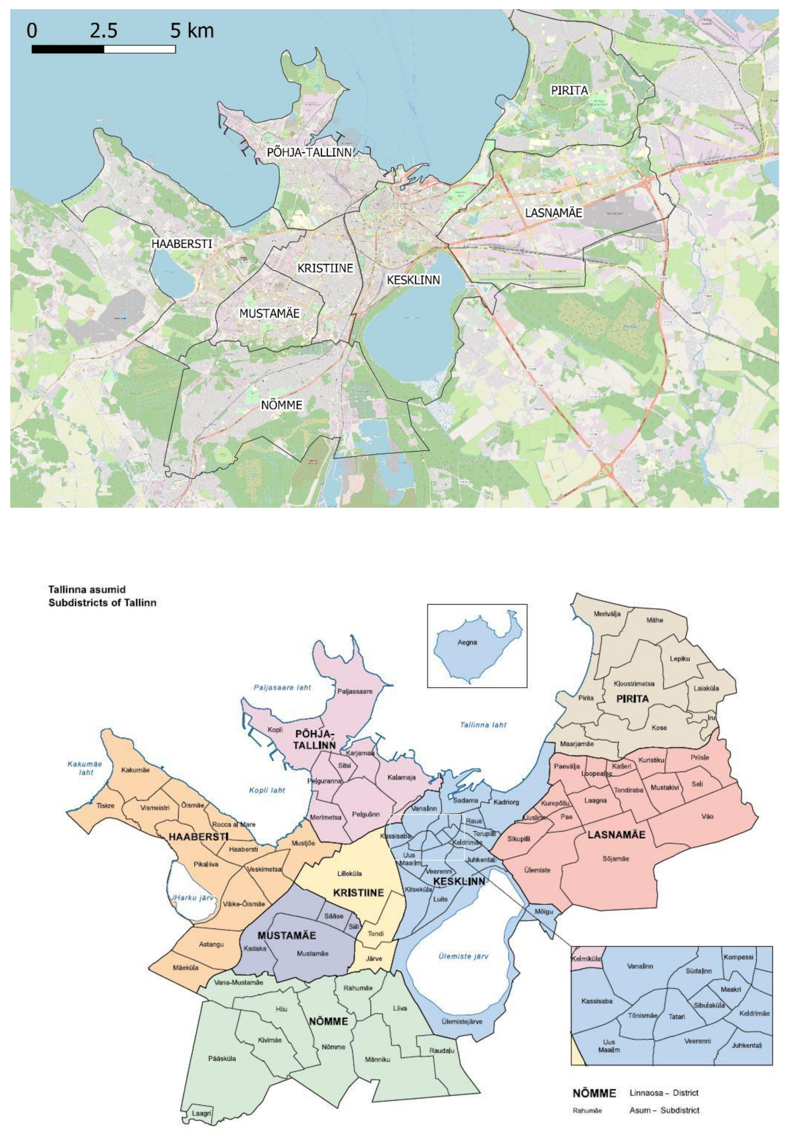
The methodology is applied here on a case study related to the city of Tallinn, Estonia. Tallinn is a European capital characterized by an efficient bus and trolleybus network and an important port that serves high flows of both freight and commuters. It is also located on one of the TEN-T axes (Rail Baltica). Maps showing districts and subdistricts are provided in Figure 3.
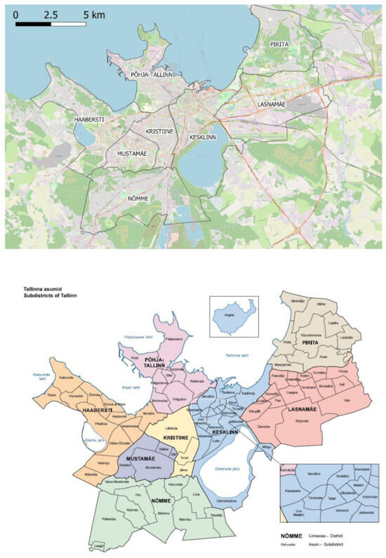
Figure 3.
Tallinn districts (top) and subdistricts (bottom). (Source: Estonian Ministry of the interior, Population Register).
The chosen reference year is 2015, motivated by the fact that a travel survey [33], which included travel diaries, was recorded during that year. In 2015, the city counted 414,000 inhabitants, the most populated among the eight districts being Lasnamäe and Mustamäe; relevant statistics and distributions, such as gender per age were obtained both from the national statistical database (www.stat.ee; accessed on 28 December 2021) or from the municipal records [34].
We report in the Appendix A an overview of all the available data that could be utilized. Essentially, all data sources were openly available for free, with the only exception of workplace aggregates that required a fee for the extraction process. It is worth highlighting that, as argued in Section 2, non-public data sources (e.g., mobile phone data, company addresses, floor space, disaggregate statistics, commuting ODs, etc.) or any data allowing for more complex assignments were not considered in this study.
The process that was followed to generate and validate the final dataset for the city of Tallinn is summarized in Figure 4, where each step is tied to the needed inputs.
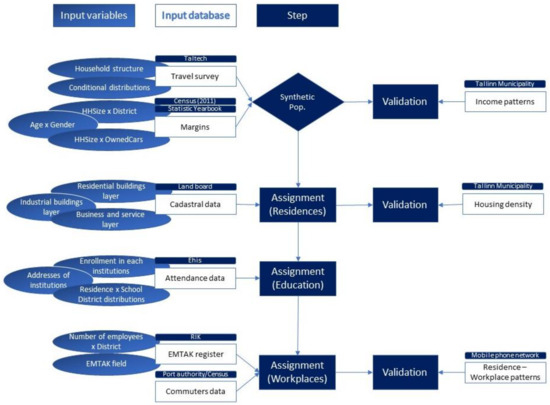
Figure 4.
Process—from synthetic population to the input dataset for an ABM.
As it can be seen in Figure 4, the work on the synthetic population follows four main phases, for each of which both the sources and the exploited variables were reported. Besides, on the right, the data used for validation were listed, again highlighting the sources. For the modeling to suggest decision making, trust in the results is very important and can be fostered through validation, a key step in every analysis, even more so when a minimum set of data is exploited as in this case. Figure 4 also tries to highlight the modular nature of the process.
3.2. General Description and Data Availability
In order to generate the synthetic population to be later assigned, the SimPop package was chosen [10]. However, it must be highlighted how the choice of SimPop does not limit the applicability of the presented approach, since basically any other method able to produce a synthetic population can be exploited to generate the needed inputs. For additional details concerning the SimPop tool, interested readers may refer to [10]. Despite this first step produces an initial version of the synthetic population, this is not yet ready to be exploited as input for an activity-based demand model, as it still lacks key variables such as places of education and workplaces. As it can be seen from Figure 1, these variables are modeled through the intermediate step “spatial assignment” and result in the key anchor points needed to replicate typical travel patterns. However, the anchor points could not be included because they were not properly captured by the travel diaries. Furthermore, the residence distribution had to be further disaggregated since each agent should be assigned to an area that would allow to model her/his mobility choices (e.g., 500 × 500 m). Indeed, it is not possible to apply choice models to areas as big as subdistricts while it is possible to do so when the degree of precision is within walking range. A more disaggregated synthetic population is found to hold the best precision while retaining good levels of accuracy (as proved in [35]).
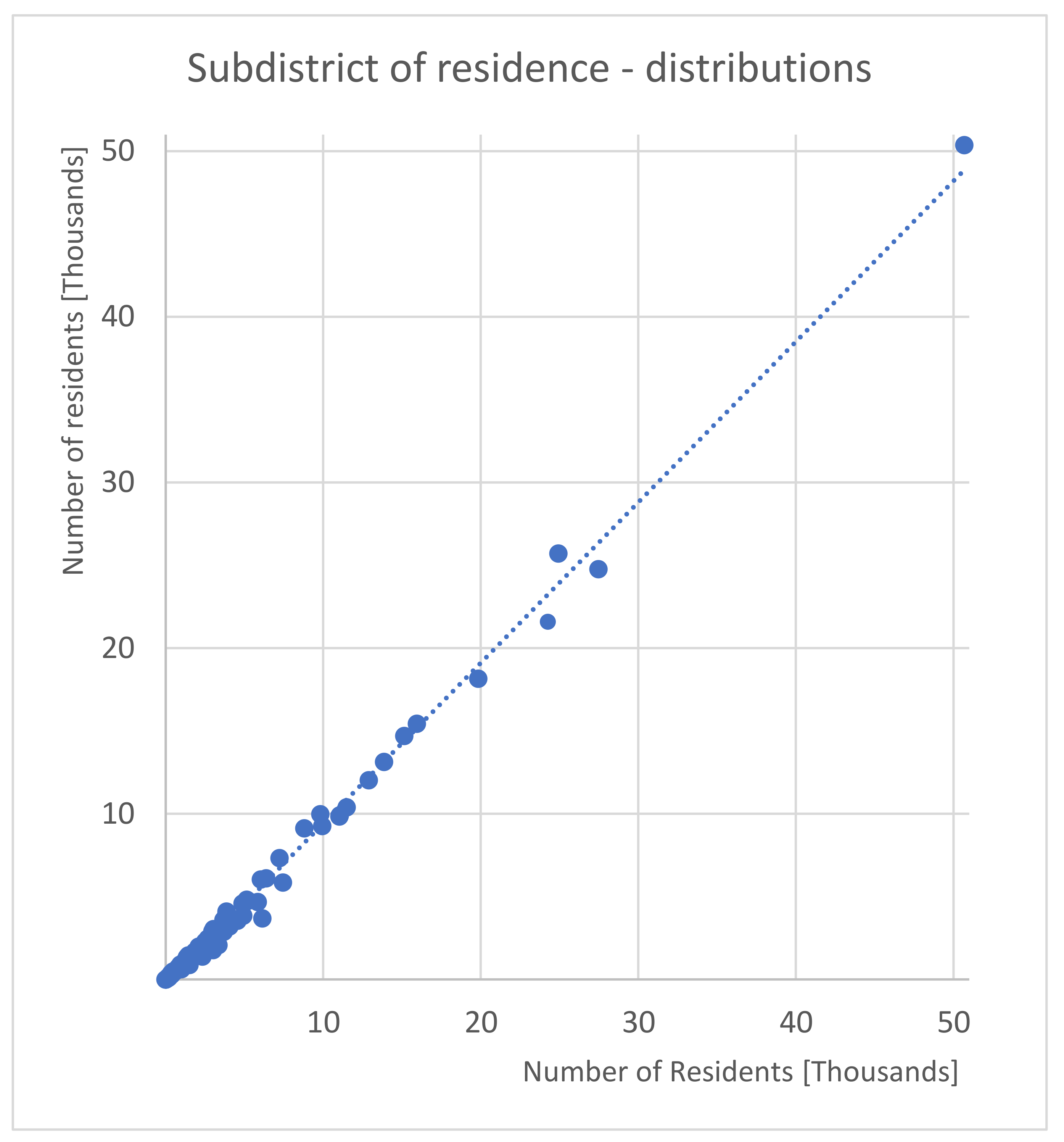
We report in Figure 5 the first version of the synthetic population resulting from applying the SimPop tool, where it may be observed that the two populations (real, i.e., from census, and synthetic) match almost perfectly in terms of household sizes and spatial distribution across Tallinn’s subdistricts. This happens indeed because the final calibration was carried out through simulated annealing on these two variables (which were deemed more important for the case study than, for example, the gender × age distribution). In addition, due to the survey structure, the average income per family member was more closely related to the household structure than to the individual. Thus, since income is another key variable for an ABM, a more precise household size distribution was favored over calibration on individual variables. More details about the synthetic population is provided in Section 4.

Figure 5.
Subdistricts population resulting from SimPop—the x-axis represents the number of residents in a subdistrict in the real population while the y-axis represents the number of residents in the synthetic population (a perfect match would result in a 45 degree trendline).
3.3. Spatial Assignment—Workplaces
To implement the spatial assignment of workplaces, an aggregated dataset was obtained from the Estonian Centre of Registers and information Systems (RIK).
Such dataset differs from the more complex ones reported in literature by being aggregated and anonymized. in fact, only the total margins for the number of employees in each EMTAK field at district level were exploited. In this section, each individual is assigned a workplace within a cell in the grid, without assigning her/him to a specific building or address. The exploited distributions are reported in Figure 6 and Figure 7.
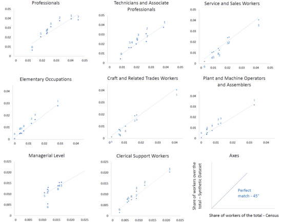
Figure 6.
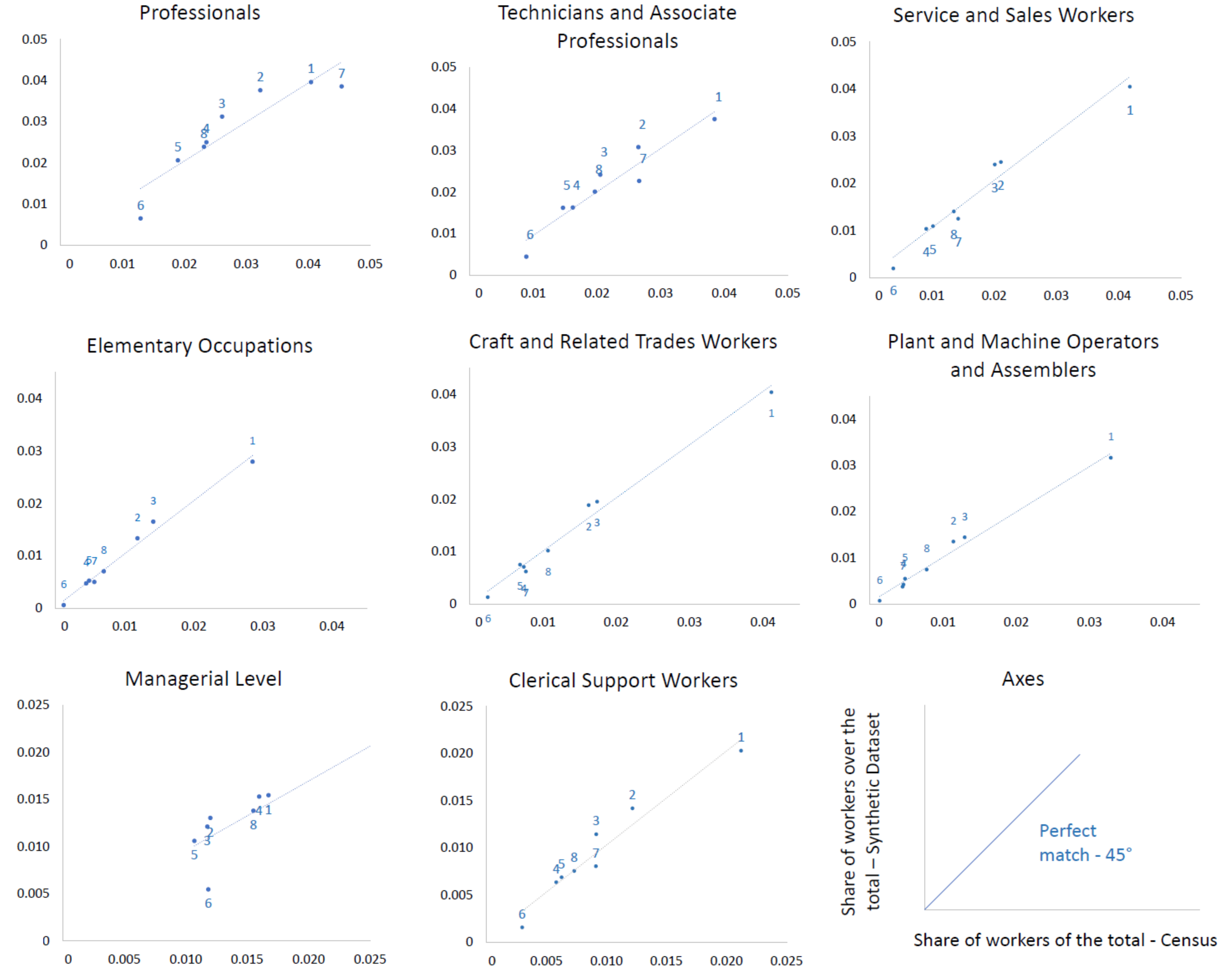
Example of different occupations and spatial distributions per district of residence (district numbered in the range 1–8). The x- and y- axis represent the percentage of jobs in each NACE category over the total. The x-axis represents the shares in the synthetic population/census, while the y-axis represents the shares in the other dataset. A perfect correspondence would result in a 45 degree trendline.
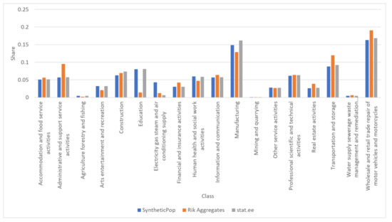
Figure 7.
EMTAK/NACE classes: synthetic population against RIK dataset and census (source: stat.ee).
In the following, the application to the Tallinn case study using the methodology described in Section 2 is presented. First, from publicly available census data, one may obtain the distributions of workers in the EMTAK field based on occupation (which, in turn, is related to gender, age, and district of residence). This is exploited to assign a field to each individual in the synthetic population, while keeping consistency in the spatial distribution of professional roles; Figure 6 reports the achieved matches among occupation and the overall population. It must be highlighted again how the synthetic population may slightly differ from the actual one in some areas or in some features. This is due to the stochastic nature of the assignment and depending on the margins the population is calibrate against. It is therefore important to verify that the margins are consistent with the census one; in this case, the occupation fields were assigned based on age, gender, and district of residence and we can conclude that the degree of consistency is satisfactory. Once the assignment of the EMTAK fields is performed, the totals in the synthetic population arising from the census data are compared with the totals in the RIK dataset and inconsistencies are identified. For example, the workers in “Education” are 14,118 in the census results, while they are only 2825 in the RIK dataset (see Figure 7). All the outliers are then categorized as “others” and their field is not exploited in assigning the workplace district; whereas, for the fields whose distribution matches between the two datasets, it is instead possible to exploit the distribution.
Once the EMTAK dataset is coherent among the RIK and the census databases, both the assignment of the EMTAK field and of the workplace district are carried out by applying the recorded distributions (as detailed in Section 2). Thus, the focus will be on the last mile, which is implemented as follows:
- First, weights based on the class of each cell are assigned, which allow also to calculate the total weight for all the cells in each district;
- Then, the ratio i between each cell weight and total of the weights in the district is calculated according to Equation (2).
For the EMTAK workers whose total are coherent between RIK data and the census, the ratio i is exploited to assign the cell of the workplace. Distance and EMTAK fields are then exploited to assign the subzone, namely the work district, which allows to frame coherent and realistic commuting patterns. For the other workers, the simple cell assignment was deemed potentially too skewed and the work district assignment was not possible a-priori based on census or EMTAK distributions.
Therefore, to avoid having individuals working on the other side of the city only based on the cell weights, the following heuristic algorithm is applied:
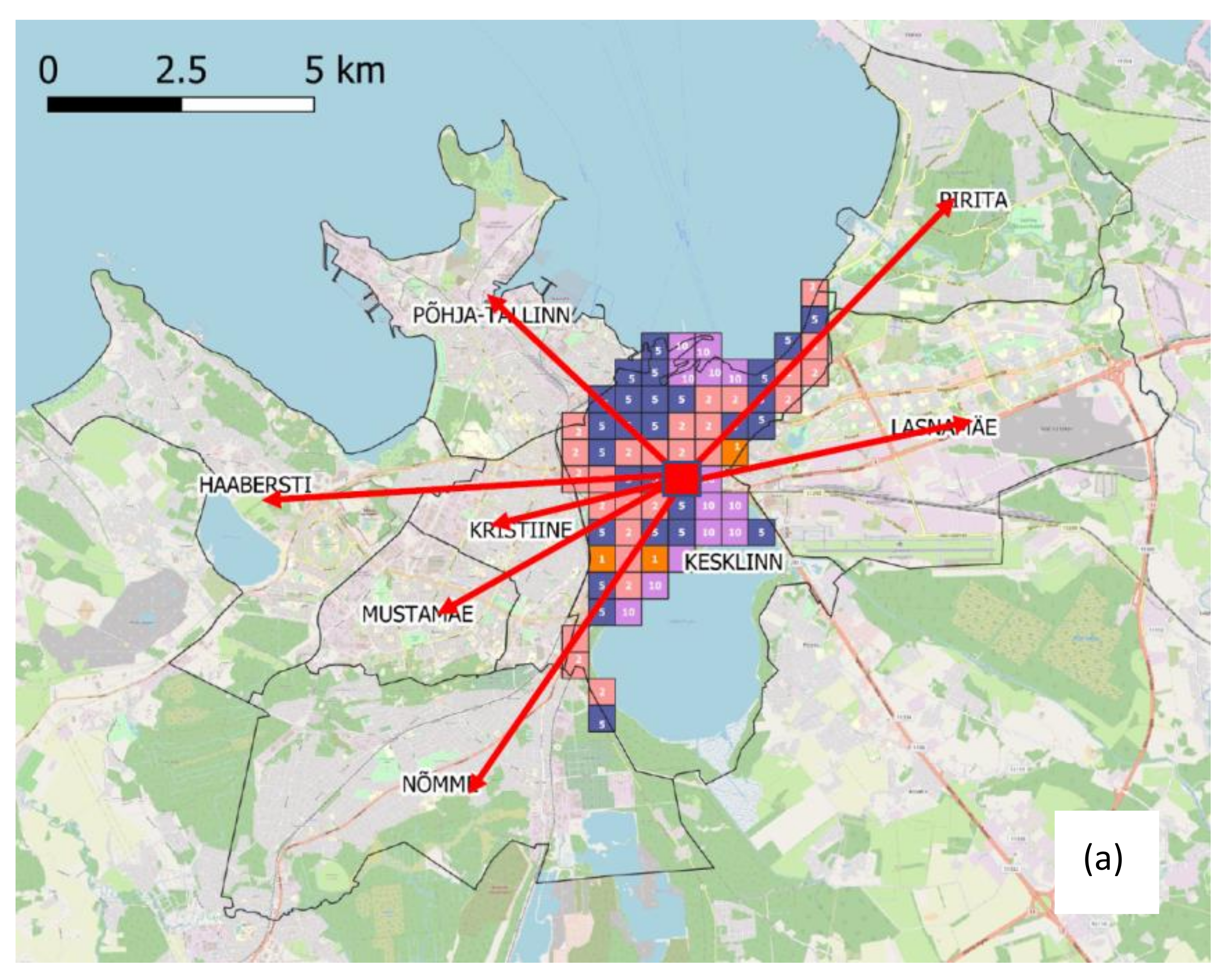
- The distance between each residence cell and each district, calculated as average between all the distances between the cell at hand and the ones included in the district, is computed (see an example in Figure 8a).
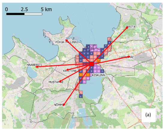
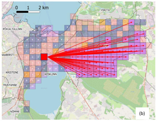 Figure 8. (a) Land use weights for Kesklinna and distances from each district for each cell; (b) last mile assignment based on distance (linear).
 - For each cell pair (one being the residence, the other being the eligible workplace), the ratio between their distance and the average distance among the residence cell and all the other cells in the district is calculated.
- Each district has its own gravitational pull calculated based on the number of employees in the remaining fields (“others”). In this case, the probability of working in a district is calculated via Equation (4). Even if a certain noise is added to the total number of jobs in the “other” field, a spatial integrity is kept (distant districts have less chances of being chosen). Besides, it will be showed how the total number of “other” employees in each district remains quite consistent.
- The class of the workplace cell is calculated based on the cell classes distribution within the district via Equation (5).
- Once both the district and the class are assigned for the workplace, the final cell assignment is simply carried out through Equation (6); Figure 8b illustrates how the final cell assignment is carried out within each class.
Note that distance as a factor is only considered as a corrective item when assigning the workplace district (the main factor being the gravitational pull of the number of jobs or the actual EMTAK distribution) and for the last mile assignment. Moreover, when assigning the work district, the distance factor is considered only for the fields of work for which no reliable spatial information was available. The above was carried out through only spatial data concerning the number of buildings in each cell and their main destination and the aggregate statistics at district level about the number of employees per EMTAK field (where possible).
Figure 8b shows the last step of the method, which involves the distance assignment. People residing in the red cell have already been assigned to the district of work based on census margins and NACE fields and to a cell class based on the relative weights and the resulting probability. Then, after the workplace has been defined as one among the purple ones, the distance is employed as final proxy. Indeed, since the purple cells fall in the manufacturing type and have a high weight, the number of workers in the distant cells on the eastern border turns out to be higher than the workers in the west and northern section of the district (the ones nearest to the red cell of residence).
4. Results
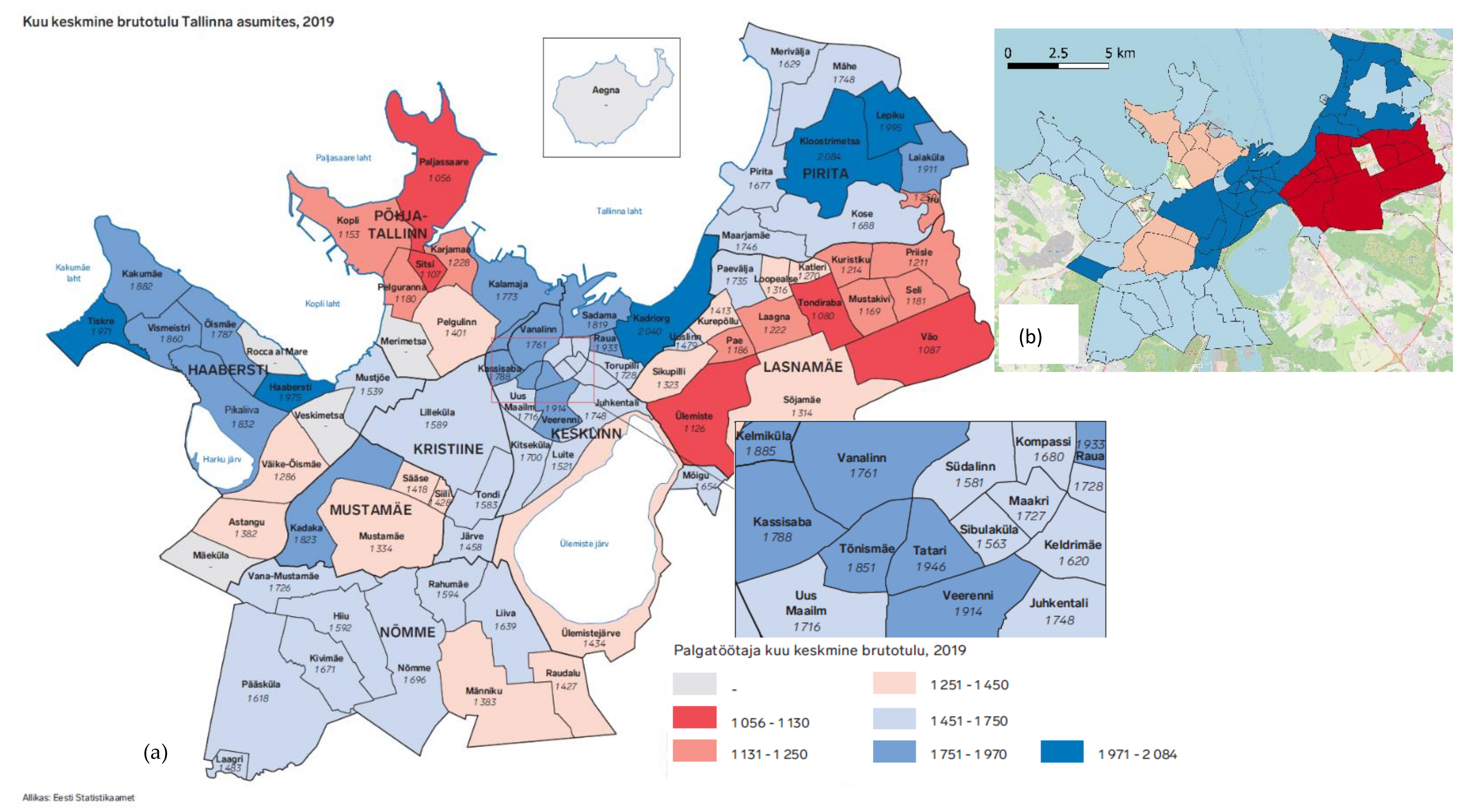
In the following, we present an overview of the relevant distributions in the final dataset and we investigate how they match real world data. As it can be seen from Figure 9, the income distribution for the synthetic population matches reasonably well, at least in qualitative terms, the real one. The only inaccuracies appear for the small subdistricts, due to the very low number of residents (a similar issue with smaller areas is also reported in [8]). To maintain the synthetic dataset anonymized, the income per family member variable was converted into four levels (high, average, low, and not available). The total number of cars was instead assigned based on the margins found in [36], following a probability distribution based on household variables.

Figure 9.
Income distribution across subdistricts: (a) real population (source: Eesti Statistika amet–edited); (b) synthetic population (dark red = lowest income, dark blue = highest income).
As mentioned, activity-based models need a level of spatial disaggregation not framed by the census data and not reproducible through tools such as SimPop. In our case study, the city of Tallinn is partitioned in 628 500 × 500 m cells, which are then categorized as highly residential (HR), low residential (LR), businesses and services type (OW), and manufacturing type (MW) based on some of the classes defined in [19], cadastral data, and the different destinations for the buildings in each cell, as shown in Figure 10.
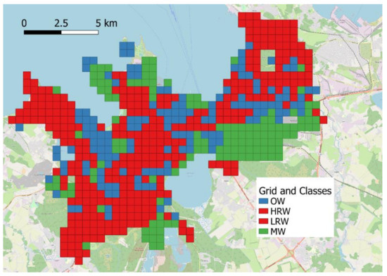
Figure 10.
Scored grid and cell classes in the city of Tallinn–OW (business/services weight), MW (manufacturing weight), LRW (lowly residential weight), and HRW (highly residential weight).
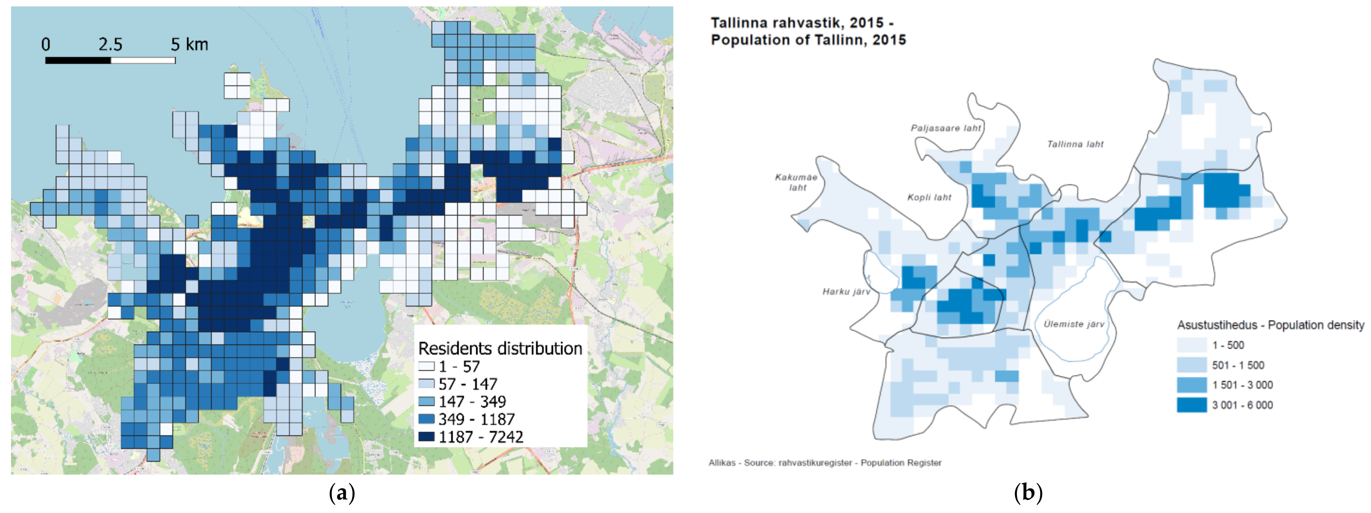
The single cell values for residents seem to precisely match the ones recorded (but not publicly shared, to the best of our knowledge) by the city census, as in Figure 11. As it may be observed, the darker blue cells in the left picture overlap with the ones in the right one.
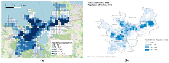
Figure 11.
Resident distribution for the synthetic population (a) and from the census ((b)—source: Rahvastikuregister).
As it can be seen in Figure 12, when combined with a realistic workplace subzone pattern, the assignment produces highly coherent patterns in the workplace distribution, which is achieved by prioritizing land use and using the distance only as a proxy to filter out unlikely combinations.
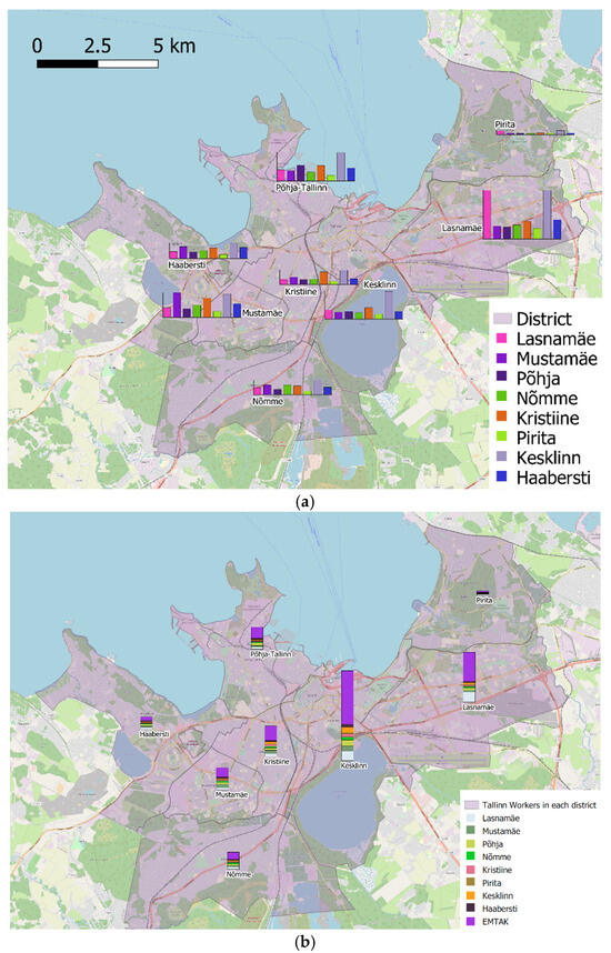
Figure 12.
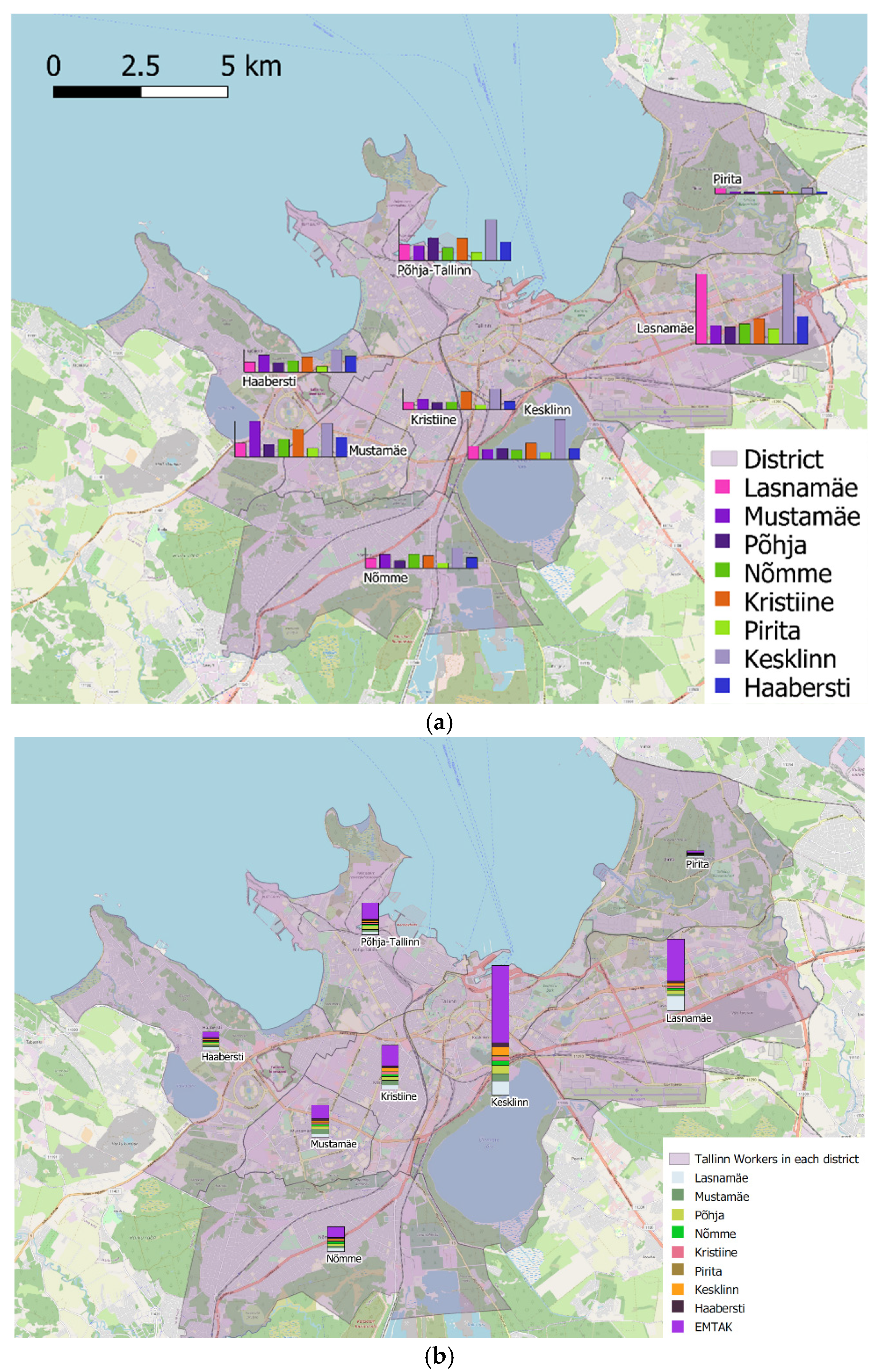
(a) Residents and their workplace district as destination; (b) workers and their districts of residence as the origin (colorcoded).
In particular, as it can be noticed from Figure 12a, the residents of Läsnamäe, for example, do work mostly in Läsnamäe and Kesklinn. The residents of Haabersti, on the other hand, tend to work in Haabersti and in Kesklinn. This captures the various trends that might be expected: the district of residence indeed attracts a fair share of workplaces while the central districts do the same. Thus, expected movements within the city are replicated while reducing skewedness to a minimum. Figure 12b aims at comparing the total of employees per district with the total per district in the resulting dataset. As it can be seen from a qualitative perspective, the assignment reproduces quite faithfully the various shares. It should be highlighted that data for a quantitative comparison are not available. The addition of the gravitational element for not coherent EMTAK fields does not skew the totals. The distribution among the cells seem to reproduce the most coherent patterns as well.
In Figure 13, the workplace cells for people residing in Nõmme and working in Põhja-Tallinna are reported. It is worth highlighting how the commuting pattern here faithfully represents the land use situation even though a gravity model was implemented. Indeed, the darker squares in the northern part represent the zones in Põhja-Tallinna where the harbor buildings are situated, while the southern darker squares are the result of the added gravitational element that capture the areas near the city center and near the train station. Besides, this pattern is specific to commuting between Põhja-Tallinna and Nõmme since the residence/work district distribution was kept through the EMTAK field assignment. This way, all the existing information are exploited for the assignment, with the gravitational hypothesis coming into play only when no other relevant information is available.
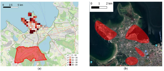
Figure 13.
Commuting patterns—darker cells being the ones with the more workplaces; (a) from assignment; (b) from Google Maps.
A final comparison is performed against [37], a recent study investigating commuting patterns in Tallinn by exploiting mobile phone cellular network data. The reference period of the study was May 2018 and the degree of precision was at district level. Note that the two studies are built on very different datasets and the raw data from the mobile phone network were not available to the authors. Table 2 provides the results obtained by both the proposed workplace assignment method and the ones reported in [37].

Table 2.
Residence/workplace pattern obtained from the workplace assignment (top) and from [37] (bottom). Each row represents an origin while each column represents a destination. Each cell represents the share of trips from the origin to the various destinations across a row. Darker colors convey a higher share of trips in that OD couple. Results from [37] were obtained through an analysis of mobile phone data.
One can observe that the hypotheses made about land use, EMTAK fields and distances frame the overall trends, even capturing outliers such as Pirita-Lasnamäe accounting for a 22% of the residing workforce. In Table 2, the percentages represent the shares of workers departing from the district of origin (rows) to reach the district of workplace (column). The percentages should be compared across rows (i.e., the sum of each row percentage results in 100%). The comparison is carried out by both comparing the visual pattern arising in Table 2 and by observing the delta arising from the two datasets. Only the distributions and not the absolute values could be compared since in [37] no absolute value is reported.
In Table 3, the difference between the percentage in Table 2 are reported. As it can be noticed, most of the differences sit below or around 5%. Still, a pattern of errors emerges for the case where workers reside and work in the same district, which are consistently higher in [37]. This may have different interpretations and the two most plausible hypotheses in the authors’ opinion are:

Table 3.
Difference of percentage (Delta %) between the results of this paper and [37].
- In this study, the weight of distance should be higher for workplaces in the immediate proximity of the habitation. This would reflect a nonlinear pattern in the relevance of distance. The distance would weigh more than the other factors (land use and EMTAK fields) for the cells in the immediate surroundings of the residence location.
- In [37], workplaces are identified as the most frequent cell-ID registered between 11:00 and 16:00 during working days. Cases in which these cell-IDs are the same as the residence ones are excluded. While this filtering probably captures most of homeworkers, retired people, and people with different work schedules (the approach is similar to other studies, such as [38]), it may fail in identifying some outliers (e.g., stay-at-home parents with a gym routine). This would result in an overestimation of the people working and residing in the same district.
The authors’ hypothesis is that the truth lies probably in between, with the approach presented in this paper failing to capture some of the preferences related to a closer workplace and the approach in [37] possibly capturing some unintended entries due to the anonymity of the data. Finally, some small discrepancy may be due to the different reference year (2015 and 2018). As mentioned in literature [37,38], while mobile phone data is a valuable source of information, the validation of resulting datasets is challenging due to lack of data. The method presented in this paper, an alternative for when mobile phone data is not available, seems to fill this gap as well.
To summarize, it was possible to validate residence and workplace patterns, the spatial distribution of various household sizes, and the distribution of gender and age within the population. Thus, each step of the process was checked against the best available data and the results were deemed promising.
5. Discussion
The presented work introduces a methodology to assign workplaces to a synthetic population employing a limited amount of aggregated data, without exploiting the more advanced data sources utilized in existing literature. Table 1 frames the difference in data requirements and the research gap this paper aims to fill, namely if and how it is feasible to carry out an assignment of anchor points while exploiting only aggregates for a population. It is important to highlight that the results are even more valuable since the commuting patterns are assigned to a resolution of 500 × 500 m.
For the Tallinn case study, it was possible to build an OD commuter pattern that satisfactorily matches the trends observed by analyzing mobile phone data (Table 2). Besides, as shown in Figure 13, establishments and workplaces were identified with good precision, basically estimating the firms’ locations instead of modeling it or receiving it as an input.
It is here argued that the limited amount of data needed for the methodology to work and the reliable results are not the only research gap the paper fills. By applying the method to a real-life case study and comparing it against another data source (Table 2) the paper proves the feasibility and reliability of the proposed solution. Effort was made to report in detail each step of the modeling pipeline and the used code and results are provided as open source. The aim in this case is to foster replicability and transferability, which were identified in Section 1 as some of the current limitations in the state-of-the-art [29]. The main advantage of the proposed method over the existing ones lies in the very light data requirement. Besides, the code made available is written in R and every step is implemented through it, so no specific requirements arise concerning computational power, operating system or memory limits. All the input data are in .csv format, so data processing complexity is not an issue; for the Tallinn case study, the code runs through the assignments in a matter of (dozens of) minutes.
It should also be highlighted how the synthetic population and the resulting assignment presented in this paper are key steps in wider analyses, as suggested in Figure 1. The ABM that may be built upon datasets, such as the presented one, can then be exploited to carry out wider assessment concerning for example traffic efficiency, modal shares, and accessibility [31]. These results can then be exploited to evaluate environmental impacts and emission levels or to forecast future scenarios, such as ones including automated driving.
While the results look encouraging and amount to a working input for ABM (they were tested on SimMobility MT), some limitations are still present and are worth being discussed. A factor that should be accounted for, while modeling, is the heuristic nature of the assignment for the NACE fields classified as “others”. Depending on the share of these workers and the commuting dynamics within the case study, the results should be carefully analyzed and possibly validated through additional metrics. This problem is less relevant when multiple data sources are exploited [11,17,25,26,27,28,29] since the validation becomes less pressing.
Moreover, the lack of more disaggregated data limited the validation that could be performed. This makes the validation of the presented method more challenging than it is in works exploiting additional data [11,17,25,26,27,28,29]. Replicating this approach to other case studies with more available data would further allow to quantify the achieved degree of precision. To apply the presented method to another case study could also allow to compare its performance against any of the methods and tools described in Section 1. Due to the nature of the Tallinn case study, namely the lack of reliable workplace entries in the household survey and the scarcity of other data (see Table 1), it was not possible to carry out any more detailed performance assessment.
Future research directions opened by this paper concern current challenges, such as the rise of flexible or remote working patterns. The addition of NACE fields should allow the modeling these patterns in parallel with the assignment of workplaces. Future works that may be carried out with the presented dataset or methodology would see the various NACE fields related to different remote working statistics and assess the ability to frame the changes in actual flows of people among the 500 × 500 m zones. Other research directions would concern the integration of the public transport stops in the weighting land use factors or focus on the weighting of the distance factor in the immediate vicinities of the residence, to investigate the discrepancies highlighted in Section 4. Finally, a limitation of the paper is that it exploits the weights reported in [19], conceived for a prototype city. Future development could investigate the presented method applied to a case study in which detailed land use data are recorded to perform a calibration of said weights. Besides, other open mobility data, such as public transport lines and skim matrices, could improve precision, i.e., by skewing the weights of certain cells close to actual mobility hubs.
6. Conclusions
The paper describes a systematic methodology to assign workplace anchor points to a synthetic population, by exploiting land use data and an aggregate dataset with totals of employees per NACE field. The resulting population is conceived to be employed for activity-based demand generation. The designed method is designed as nimble, modular (i.e., not bound to any existing tool), and reliant on mostly open and/or aggregate datasets. The contribution should then make easier to exploit agent-based models and further foster their uptake both in scientific literature and professional setups. The described solution is replicable and highly transferable, with the main strength lying in its simplicity and low reliance on available data. In particular, the transferability is ensured by the fact that the proposed methodology exploits only open data in the format commonly registered by national or supranational statistical bodies and that no foreseeable barrier may be identified a priori. The filled research gap involves the lack of workplace assignment methods for synthetic populations, based on very scarce and aggregate data. This paper details each passage of such a method and tests it on a real city, validating the results and assessing the reached level of precision. The resulting dataset is detailed to be exploitable by fellow researchers for activity-based modeling (or any other research direction) since it is shared as open source at: https://github.com/Angelo3452/Tallinn-Synthetic-Population. Additional details are provided in the Data Availability Statement section.
Author Contributions
Conceptualization, Serio Agriesti, Claudio Roncoli and Bat-hen Nahmias-Biran; methodology, Serio Agriesti, Claudio Roncoli, and Bat-hen Nahmias-Biran; validation, Serio Agriesti; formal analysis, Serio Agriesti, Claudio Roncoli, and Bat-hen Nahmias-Biran; data curation, Serio Agriesti; writing—original draft preparation, Serio Agriesti, Claudio Roncoli; writing—review and editing, Serio Agriesti, Claudio Roncoli, and Bat-hen Nahmias-Biran; visualization, Bat-hen Nahmias-Biran, Serio Agriesti, and Claudio Roncoli; funding acquisition, Claudio Roncoli. All authors have read and agreed to the published version of the manuscript.
Funding
This research was funded by the FINEST Twins Center of Excellence, H2020 European Union funding for Research and Innovation grant number 856602.
Institutional Review Board Statement
Not applicable.
Informed Consent Statement
Not applicable.
Data Availability Statement
Data exploited as statistical margins may be found at stat.ee (from the census) or on the city of Tallinn website (statistical yearbooks: https://www.tallinn.ee/eng/Statistics-and-yearbooks; accessed on 28 December 2021). Data exploited for validation may be found in [37]. The Tallinn synthetic population dataset is available at: https://github.com/Angelo3452/Tallinn-Synthetic-Population. It is open source and licensed under Creative Commons—Attribution 4.0 International—CC BY 4.0. Its structure and the provided variables are there described, while additional relevant distributions are reported. Two examples implementing the methodology described in this paper are also included, written in the programming language R.
Acknowledgments
The authors would like to thank Dago Antov from TalTech for sharing the travel survey exploited in this work. Moreover, the authors are grateful to the Tallinn Municipality and to all of the related public bodies who supported this research by sharing data. Finally, the authors would like to thank all of the partners and stakeholders involved in the FinEst Twins Centre of Excellence.
Conflicts of Interest
The authors declare no conflict of interest.
Appendix A
| Data | Type of Data | Source | Usage | Public/Private |
| Household structure | Survey data | Survey from TalTech | Synthetic Population | Private |
| Age × gender distribution | Statistical margin | Statistical Yearbook of Tallinn | Synthetic Population | Public |
| Household size × district distribution | Statistical margin | Statistical Yearbook of Tallinn | Synthetic Population | Public |
| Population × subdistrict | Statistical margin | Statistical Yearbook of Tallinn | Synthetic Population | Public |
| Car Ownership × household size | Probability distribution | Survey from TalTech | Synthetic Population | Private |
| Income per family member × subdistrict | Distribution | Municipality of Tallinn | Validation | Upon request |
| Residential buildings × cell (m2) | Land Use | Tallinn Geoportal | Weight assignment | Public |
| Manufacturing and industrial buildings × cell (m2) | Land Use | Tallinn Geoportal | Weight assignment | Public |
| Service and office buildings × cell (m2) | Land Use | Tallinn Geoportal | Weight assignment | Public |
| Enrollment × educational building | Assignment | EHIS database (https://enda.ehis.ee/avalik/avalik/oppeasutus/OppeasutusOtsi.faces: database of educational institutions and enrollment statistics; accessed on 10 December 2020) | Spatial assignment | Public |
| Location of each educational building | Assignment | EHIS database | Spatial assignment | Public |
| Classification of each educational building | Assignment | EHIS database | Spatial assignment | Public |
| District of residence × enrollments in each district | Assignment | EHIS database | Spatial assignment | Upon request |
| Number of employees × district × EMTAK field | Assignment | RIK | Spatial assignment | Publicly available for a fee |
| Gender, age, and district of residence × occupation | Assignment | Census | Spatial assignment | Public |
| Occupation × EMTAK field | Assignment | Census | Spatial assignment | Public |
| Household structure | Survey data | Survey from TalTech | Synthetic population | Private |
| Age × gender distribution | Statistical margin | Statistical Yearbook of Tallinn | Synthetic population | Public |
| Household size × district distribution | Statistical margin | Statistical Yearbook of Tallinn | Synthetic population | Public |
References
- Schrank, D.; Eisele, B.; Lomax, T. 2019 Urban Mobility Report. Available online: https://mobility.tamu.edu/umr/report/#methodology (accessed on 23 July 2021).
- Brannigan, C.; Biedka, M.; Hitchcock, G. Study on Urban Mobility—Assessing and Improving the Accessibility of Urban Areas Final Report and Policy Proposals. Available online: https://ec.europa.eu/transport/themes/urban/news/2017-04-07-study-urban-mobility-%E2%80%93-assessing-and-improving-accessibility-urban_en (accessed on 23 July 2021).
- Lozzi, G.; Marcucci, E.; Gatta, V.; Rodrigues, M.; Teoh, T.; Ramos, C.; Jonkers, E. Sustainable and Smart Urban Transport. Policy Department for Structural and Cohesion Policies Directorate—General for Internal Policies PE. Available online: https://www.europarl.europa.eu/RegData/etudes/STUD/2020/652211/IPOL_STU(2020)652211_EN.pdf (accessed on 23 July 2021).
- United Nations Department of Economic and Social Affairs, Popular Division. The World’s Cities in 2018. Available online: https://digitallibrary.un.org/record/3799524 (accessed on 23 July 2021).
- Benevolo, C.; Dameri, R.P.; D’Auria, B. Smart mobility in smart city: Action taxonomy, ICT intensity and public benefits. In Empowering Organizations; Lecture Notes in Information Systems and Organisation; Springer: Cham, Switzerland, 2016; Volume 11. [Google Scholar]
- Kagho, G.O.; Balac, M.; Axhausen, K.W. Agent-Based Models in Transport Planning: Current State, Issues, and Expectations. Procedia Comput. Sci. 2020, 170, 726–732. [Google Scholar] [CrossRef]
- Nahmias-Biran, B.-H.; Oke, J.B.; Kumar, N.; Lima Azevedo, C.; Ben-Akiva, M. Evaluating the impacts of shared automated mobility on-demand services: An activity-based accessibility approach. Transportation 2020, 48, 1613–1638. [Google Scholar] [CrossRef]
- Moreno, A.T.; Moeckel, R. Population synthesis handling three geographical resolutions. ISPRS Int. J. Geo-Inf. 2018, 7, 174. [Google Scholar] [CrossRef]
- Hafezi, M.H.; Habib, M.A. Synthesizing population for microsimulation-based integrated transport models using atlantic canada micro-data. Procedia Comput. Sci. 2014, 37, 410–415. [Google Scholar] [CrossRef][Green Version]
- Templ, M.; Meindl, B.; Kowarik, A.; Dupriez, O. Simulation of synthetic complex data: The R package simPop. J. Stat. Softw. 2017, 79, 1–38. [Google Scholar] [CrossRef]
- Zhu, Y.; Ferreira, J. Synthetic population generation at disaggregated spatial scales for land use and transportation microsimulation. Transp. Res. Rec. 2014, 2429, 168–177. [Google Scholar] [CrossRef]
- Konduri, K.C.; You, D.; Garikapati, V.M.; Pendyala, R.M. Enhanced Synthetic Population Generator That Accommodates Control Variables at Multiple Geographic Resolutions. Transp. Res. Rec. 2016, 2563, 40–50. [Google Scholar] [CrossRef]
- Yaméogo, B.F.; Gastineau, P.; Hankach, P.; Vandanjon, P. Comparing Methods for Generating a Two-Layered Synthetic Population. Transp. Res. Rec. 2021, 2675, 136–147. [Google Scholar] [CrossRef]
- Lenormand, M.; Deffuant, G. Generating a synthetic population of individuals in households: Sample-free vs sample-based methods. J. Artif. Soc. Soc. Simul. 2013, 16, 12. [Google Scholar] [CrossRef]
- McBride, E.C.; Davis, A.W.; Lee, J.H.; Goulias, K.G. Incorporating land use into methods of synthetic population generation and of transfer of behavioral data. Transp. Res. Rec. 2017, 2668, 11–20. [Google Scholar] [CrossRef]
- Cajka, J.C.; Cooley, P.C.; Wheaton, W.D. Attribute Assignment to a Synthetic Population in Support of Agent-Based Disease Modeling. Methods Rep. RTI Press 2010, 19, 1–14. [Google Scholar] [CrossRef] [PubMed]
- Le, D.T.; Cernicchiaro, G.; Zegras, C.; Ferreira, J. Constructing a Synthetic Population of Establishments for the Simmobility Microsimulation Platform. Transp. Res. Procedia 2016, 19, 81–93. [Google Scholar] [CrossRef]
- Erath, A.L.; Fourie, P.J.; Sun, L.; Vitins, B.J.; Atizaz, A.; van Eggermond, M.A.B.; Ordóñez Medina, S.A. MATSim Singapore Synthetic population and work locations. In Proceedings of the Urban Redevelopment Authority (URA) Planning Analytics Symposium, Singapore, 3 May 2016. [Google Scholar]
- Oke, J.; Akkinepally, A.; Chen, S.; Xie, Y.; Aboutaleb, Y.M.; Lima Azevedo, C.; Zegras, C.; Ferreira, J.; Ben-Akiva, M.; Shaheen, S.; et al. Evaluating the systemic effects of automated on-demand services via large-scale agent-based simulation of auto-dependent prototype cities. Transp. Res. Part A Policy Pract. 2020, 140, 98–126. [Google Scholar] [CrossRef]
- Ortúzar, J.; Willumsen, L.G. Trip Distribution Modelling. In Modeling Transport, 4th ed.; John Wiley & Sons: Hoboken, NJ, USA, 2011. [Google Scholar]
- Gallagher, S.; Richardson, L.F.; Ventura, S.L.; Eddy, W. SPEW: Synthetic Populations and Ecosystems of the World. J. Comput. Graph. Stat. 2018, 27, 773–784. [Google Scholar] [CrossRef]
- Ge, Y.; Meng, R.; Cao, Z.; Qiu, X.; Huang, K. Virtual city: An individual-based digital environment for human mobility and interactive behavior. SIMULATION 2014, 90, 917–935. [Google Scholar] [CrossRef]
- Bodenmann, B.R.; Vecchi, I.; Sanchez, B.; Bode, J.; Zeiler, A.; Axhausen, K.W. Implementation of a Synthetic Population for Switzerland. IVT, ETH Zurich. 2017. Available online: https://www.research-collection.ethz.ch/handle/20.500.11850/104334 (accessed on 28 December 2021).
- Wang, L.; Waddell, P.; Outwater, M.L. Incremental Integration of Land Use and Activity-Based Travel Modeling: Workplace Choices and Travel Demand. Transp. Res. Rec. 2011, 2255, 1–10. [Google Scholar] [CrossRef]
- Fournier, N.; Christofa, E.; Akkinepally, A.P.; Azevedo, C.L. Integrated population synthesis and workplace assignment using an efficient optimization-based person-household matching method. Transportation 2021, 48, 1061–1087. [Google Scholar] [CrossRef]
- Balac, M.; Hörl, S. Synthetic population for the state of California based on open-data: Examples of San Francisco Bay area and San Diego County. In Proceedings of the Transportation Research Board 100th Annual Meeting, Washington, DC, USA, 21–29 January 2021. [Google Scholar]
- Wheaton, W.D.; Cajka, J.C.; Chasteen, B.M.; Wagener, D.K.; Cooley, P.C.; Ganapathi, L.; Roberts, D.J.; Allpress, J.L. Synthesized Population Databases: A US Geospatial Database for Agent-Based Models. Methods Rep. RTI Press 2009, 2009, 905. [Google Scholar]
- Wang, H.; Zeng, W.; Cao, R. Simulation of the Urban Jobs—Housing Location Selection and Spatial Relationship Using a Multi-Agent Approach. ISPRS Int. J. Geo-Inf. 2021, 10, 16. [Google Scholar] [CrossRef]
- Hörl, S.; Balac, M. Synthetic Population and travel demand for Paris and Île-de-France based on open and publicly available data. Transp. Res. Part C Emerg. Technol. 2021, 130, 103291. [Google Scholar] [CrossRef]
- Sallard, A.; Balać, M.; Hörl, S. A Synthetic Population for the Greater São Paulo Metropolitan Region.IVT, ETH Zurich. 2020. Available online: https://www.research-collection.ethz.ch/handle/20.500.11850/429951 (accessed on 28 December 2021).
- Ziemke, D.; Kaddoura, I.; Nagel, K. The MATSim open Berlin scenario: A multimodal agent-based transport simulation scenario based on synthetic demand modeling and open data. Procedia Comput. Sci. 2019, 151, 870–877. [Google Scholar] [CrossRef]
- McBride, E.C.; Davis, A.W.; Goulias, K.G. A Spatial Latent Profile Analysis to Classify Land Uses for Population Synthesis Methods in Travel Demand Forecasting. Transp. Res. Rec. 2018, 2672, 158–170. [Google Scholar] [CrossRef]
- Triinu, O. Liikumisviiside Uuring Elektrisõidukite ja Säästva Transpordi Kasutamise Arendamiseks, Tallinn, Estonia. 2015.
- Tallinn City Government Tallinn Arvudes 2015. Statistical Yearbook of Tallinn; Tallinn City Office: Tallinn, Estonia, 2015. [Google Scholar]
- Khachman, M.; Morency, C.; Ciari, F. Impact of the Geographic Resolution on Population Synthesis Quality. ISPRS Int. J. Geo-Inf. 2021, 10, 790. [Google Scholar] [CrossRef]
- Cavoli, C. CREATE—City Report Tallinn, Estonia. Available online: http://www.create-mobility.eu/create/resources/general/download/CITY-REPORT-Tallinn-WSWE-AV3MMA (accessed on 23 July 2021).
- Hadachi, A.; Pourmoradnasseri, M.; Khoshkhah, K. Unveiling large-scale commuting patterns based on mobile phone cellular network data. J. Transp. Geogr. 2020, 89, 102871. [Google Scholar] [CrossRef]
- Zhang, X.; Gao, F.; Liao, S.; Zhou, F.; Cai, G.; Li, S. Portraying Citizens’ Occupations and Assessing Urban Occupation Mixture with Mobile Phone Data: A Novel Spatiotemporal Analytical Framework. ISPRS Int. J. Geo-Inf. 2021, 10, 392. [Google Scholar] [CrossRef]
Publisher’s Note: MDPI stays neutral with regard to jurisdictional claims in published maps and institutional affiliations. |
© 2022 by the authors. Licensee MDPI, Basel, Switzerland. This article is an open access article distributed under the terms and conditions of the Creative Commons Attribution (CC BY) license (https://creativecommons.org/licenses/by/4.0/).

