Abstract
A terrain skeleton determines the overall structure and characteristics of the terrain and indicates the presence of significant terrain features, such as ridges and valleys. It plays an important role in terrain representation and reconstruction, hydrological analysis of watersheds, and other scientific studies and engineering applications. Previous studies of terrain skeleton have been mostly focused on the extraction of terrain skeletons, ignoring their important effect on terrain analysis. Therefore, this work proposes a new terrain skeleton, which includes three types of terrain skeleton points and two types of terrain skeleton lines. The terrain control points are peak, saddle, and valley nodes, while the terrain skeleton lines are connection lines of peaks and saddles and connection lines of saddles and valley nodes. The terrain skeleton connects isolated terrain control points together. The data structure is designed, and three analysis indicators, namely, nearest-neighbor index, topological connectivity index and landscape shape index are selected. Results show that the three selected indicators can reflect the spatial structure of the terrain skeleton and describe the landform development to a certain extent. Different areas of the same landform, such as the two sample areas in Shenmu County, show variations.
1. Introduction
The formation of the terrain skeleton affects the overall structure and characteristics of the terrain, and it is the controlling link in the description of the terrain’s morphological structure and formation [1,2,3]. A terrain skeleton indicates the presence of significant terrain features, such as ridges and valleys [4,5], which are the dividing lines of mountain topography. Terrain skeleton plays an important role in terrain representation and reconstruction [6,7], recognition and classification of landform types, and topography and geomorphology analysis [8].
The terrain skeleton includes different topographic features, such as peaks, saddles, ridges, and valleys. Many studies have been conducted on the extraction of terrain control points [9], including local height-difference comparison method [10,11], mathematical surface fitting method [12] and runoff simulation method [13,14]. The extraction of ridges and valleys, which as two important terrain feature lines have aroused widespread concern. Tang classified these methods according to data sources and algorithm principles [15]. The methods can be divided into contour-based methods [4,16,17], irregular triangulation-based methods [18,19], regular grid-based methods [20,21,22,23], and laser point cloud-based methods [24] based on the different data sources. Meanwhile, there are methods based on terrain surface flow direction analysis [25], image processing technology [22,26], surface geometry analysis [20,27], and the combination of the terrain surface geometry analysis and flow physical simulation analysis according to the different algorithm principles [28,29].
Although different types of terrain skeleton feature can be extracted by the various existing methods, reconstruction of the spatial relationship between the features is still challenging. The topographic features are not independent individuals, but an entirety in a certain landform. A terrain skeleton consists of not only the topographic features, but also the spatial relationship between them. The terrain skeleton struggles to represent the characteristics of landform evolution without the spatial relationship. Some researches treat the ridge and valley lines as one for research and extraction, making it impossible to analyze the results [4,23,30,31]. Chen et al. extended the analysis of skeleton using ridge line gradation based on the tree structure model, which can correctly reflect the topographic feature [32]. However, only ridge lines were included in the terrain skeleton and a deeper analysis of terrain skeleton was lacking in this work.
A certain number of topographic feature points determine the overall skeleton node of the terrain, and the topographic feature line constitutes the control line of the topographic morphology structure. The two interact and jointly control the overall structure of the terrain, resulting in a unique topographic shape. This study aims to: (1) develop a method for the reconstruction of a terrain skeleton by considering the relationships of skeleton features; and (2) analyze the characteristics of the terrain skeleton in the northern Loess Plateau of Shaanxi province, China.
2. Materials and Methods
2.1. Study Area
The study area is located in the Loess Plateau of northern and middle Shaanxi Province in China, which is a complex geomorphology formed by severe water and wind erosions. It is the core area of Loess plateau, with an area of 92,500 km2, covering with thick Loess, and generating many gullies and steep slopes on the surface. The elevation ranges from 318 to 3410 m. The Loess cover thickness gradually increases from north to south with a range of approximately 50–200 m [33]. Figure 1 shows the terrain of Loess Plateau of northern Shaanxi is high in the northwest and low in the southeast.
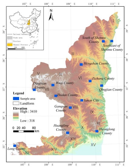
Figure 1.
Spatial distribution of the sample areas in the Loess Plateau of northern Shaanxi. (I) Loess hill and Loess ridge; (II) aeolian sand dunes to Loess hill and Loess ridge; (III) aeolian sand dunes; (IV) aeolian sand dunes to Loess tableland; (V) wind-depositional and pluvial frontal mountain Loess flatland; (VI) Loess hill; (VII) Loess ridge; (VIII) Loess-covered middle mountain; (IX) middle altitude Loess fragmented tableland; (X) Loess tableland; (XI) Loess-covered moderate relief middle mountain; (XII) Loess-covered middle mountain and intermountain Loess flatland; (XIII) Loess-covered mild middle mountain and Loess tableland; (XIV) low altitude Loess fragmented tableland; (XV) alluvial valley plain and Loess low terrace.
2.2. DEM Data of Sample Regions
It is indispensable to select typical sample areas for analysis due to the difficulty of obtaining high-resolution DEM data covering the whole study area. Therefore, the typical landforms should be picked out. Li et al. classified the landform of this area based on the catchment boundary profiles and unsupervised classification method (hereinafter referred to as the CBP-based division method) [34]. The landforms with big area and distinct topological skeleton characteristics were chosen. Then the DEMs were chosen to analyze the differences within and between landforms.
The study employed DEMs (Digital Elevation Model) with 5 m resolution and 3.3 m vertical accuracy of 13 sample areas (Figure 2), generated by interpolating the contours of 1:10,000 topographic maps and elevation points from the aerial image through photogrammetry [35]. The contours and elevation points were first used to generate a TIN data. Then the TIN was converted into grid DEM by interpolation. The DEM data were from the National Administration of Surveying, Mapping, and Geoinformation of China. A relatively complete mountain as large as possible was selected as the test data for each sample area, with valley lines as the boundary. The specific information of the areas is provided in Table 1. In each sample region, terrain control points, and terrain skeleton lines will be extracted, a terrain skeleton will be built, and the quantitative indicator results will be calculated.
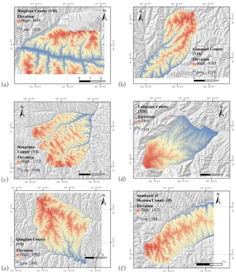
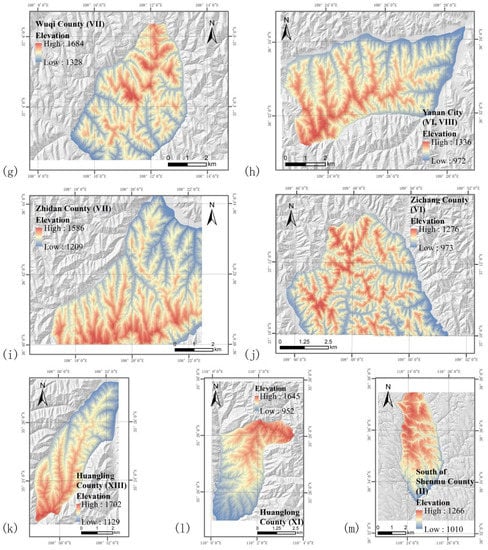
Figure 2.
DEM data of 13 sample areas. (a) DEM of Dingbian County with Loess ridge landform; (b) DEM of Ganquan Count with Loess-covered middle mountain landform; (c) DEM of Hengshan County with Loess hill landform; (d) DEM of Longxian County with Loess-covered middle mountain and intermountain Loess flatland landform; (e) DEM of Qingjian County with Loess hill landform; (f) DEM of southeast of Shenmu County with Aeolian sand dunes to Loess hill and Loess ridge landform; (g) DEM of Wuqi County with Loess ridge landform; (h) DEM of Yanan city with Loess hill and Loess-covered middle mountain; (i) DEM of Zhidan County with Loess ridge landform; (j) DEM of Zichang County with Loess hill landform; (k) DEM of Huangling County with Loess=covered mild middle tableland landform; (l) DEM of Huanglong County with Loess0covered moderate relief middle mountain landform; (m) DEM of South of Shenmu County with Aeolian sand dunes to Loess hill and Loess ridge landform.

Table 1.
Overview of selected sample areas.
2.3. Method
2.3.1. Extraction of Terrain Control Points
- Peak
The peak of the mountain refers to the highest point of elevation in the local area [36]. Its cross-sections in all directions are convex [37]. The common methods of extraction are the cross-section elevation extreme value method [38] and the local elevation difference comparison method [10]. However, the extraction result is unsatisfied due to the influence of terrain error and amplitude. Chen et al. combined closed contour lines based on window analysis to identify and isolate the pseudo peak in their improved method [39]. Existing peak extraction methods have good applicability in mountain and hilly areas, but not in some complex areas.
In geography, a mountain refers to a highland with a steep slope, where the altitude is greater than 500 m, and the relative amplitude is more than 200 m [40]. Gu established a peak extraction model based on the maximum fluctuation threshold in accordance with the terrain morphological the feature of peak based on the concept of mountain [41]. It has a high application value because the extracted results of peaks in accordance with the actual relief. Therefore, Gu’s method has been used to complete the peak accurate extraction.
- 2.
- Saddle
The saddle is the area of mild terrain with a saddle form between two adjacent mountains, and the intersection of ridge and valley lines. It is located between two peaks of mountains, and constrained by terrain trends [37,42]. The most common method for extracting saddle points is to set a moving analysis window based on DEM [43,44,45]. This method is limited by the size of analysis window, making it difficult to estimate the overall terrain changes, and it has a lot of noise and poor result accuracy.
The position of the saddle area can be clearly known with the help of the topological spatial relationship of contour lines. Wu et al. used the spatial topological relationship of contour lines to find the contour surface formed by two adjacent contour lines where the saddle point is located, and to obtain the saddle point, which is the intersection point or midpoint of the intersecting line of the central axis of the contour surface [46]. This method excludes the influence of the analysis window size. Accordingly, the extracted results are highly accurate. Therefore, Wu’s method has been used to extract saddles in this work.
- 3.
- Valley node
The valley point refers to the intersection area between different rivers in the same watershed, which can reflect the morphological characteristics and internal information of the watershed unit. This point includes ditch head points and river meeting points. In this work, the ditch head points are removed, and the river meeting points are left to build a terrain skeleton.
The extraction method of valley nodes adapts hydrological analysis, according to the single-flow D8 algorithm based on DEM data, which has a high public acceptance [47,48,49].
2.3.2. Extraction of Terrain Skeleton Lines
- Connection of peaks and saddles
The D8 algorithm is not applicable because the saddle point is not a point on the flow path starting from the peak point. We use an anti-D8 algorithm, which is a method to find the peak point from the saddle point upward to connect the saddle and peak points (Figure 3). The raster row and column of the vector peak and saddle points were recorded. A 3 × 3 window centered on a saddle point was transverse, the maximum value in the window was selected, and the grid where the maximum value is located was selected as the canter grid for the net traversal. Traversing was halted when the grid with the peak point was reached, and the algorithm terminated. The connection result is a raster that requires certain operations such as unique value display, reclassification, and turning grid to polyline, and before obtaining the vector connection lines.
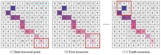
Figure 3.
Connection principle analysis diagram.
Local bumps and depressions can be observed in the terrain data due to the quality of DEM data. Accordingly, flat triangles are more likely to emerge on ridges, valleys, and mountain top areas, causing the recursive algorithm to fail because it cannot find a value larger than the central grid in 3 × 3 window (Figure 4a). Therefore, we need to eliminate the flat triangles before running the above anti-D8 algorithm(Figure 4b, [50]).
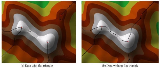
Figure 4.
Connection result of peaks and saddles.
- 2.
- Connection of saddles and valley points
The connection between the saddle point and the valley node can be realized by using the D8 algorithm. The nearest ditch point in the catchment area along the water flow direction is determined and connected with the saddle point as the canter, and the downstream valley node is connected according to the extracted water flow path. However, a saddle point is on the catchment boundary line, which have two catchments on both sides (Figure 5). A saddle point should connect the valley nodes on both sides at the same time.
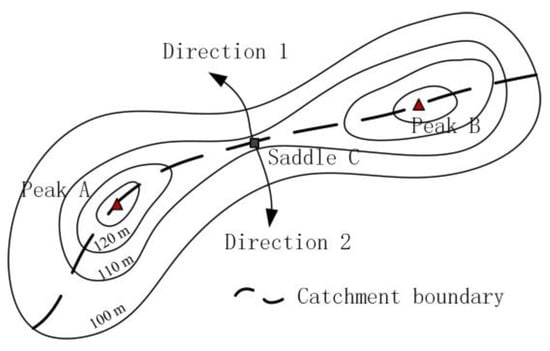
Figure 5.
Saddle point with two connection directions.
A buffer was set for the saddle point to realize the saddle and valley points in the catchments on both sides and to obtain spatial connection between the saddle point and the neighboring catchments with the overlap relationship between them. Then, a grid in each of the buffer area on both sides is selected, and it is taken as the center grid to find the minimum value in the 3 × 3 window according to the D8 algorithm. We continue to traverse with the minimum grid as the center to find a ditch point with water flow direction, eventually connecting the downstream valley node. This method is used to connect the same saddle point to valley node in the catchment area on the other side. The connection result is a raster that requires operations, and it is the same as the peak and saddle connection results, eventually obtaining the vector connection lines.
2.3.3. Reconstruction of Terrain Skeleton
After completing the extraction of terrain control points and the connection of terrain skeleton lines, a data structure used to represent the complete terrain skeleton is designed as follows:
Point: ID (index number), Z_value (elevation of point), Waviness (altitude of point), Type (type of point);
Connect_line: ID (index number), Type (type of polyline), Strat_node (starting node of connect polyline), End_node (end node of connect polyline), Length (length of polyline).
The point types include the peak, saddle, and valley node. If the point type is peak, then the altitude field must have a value, otherwise the value is −9999. The polyline types include the connecting line of the peak and saddle points and connect line of the saddle and valley points. This data structure was used to save the extracted terrain control points and terrain feature lines to complete terrain skeleton analysis later.
2.3.4. Analysis Indicators of Terrain Skeleton
The terrain skeleton is an important tool for the division of landform types in quantitative analysis. Spatial analysis includes seven directions: spatial distribution, spatial form, spatial, location, spatial similarity, spatial topology, spatial distance, and spatial correlation. These aspects should be considered when selecting analysis indicators to ensure the rationality of result analysis [25].
The analysis of the terrain skeleton was considered from three aspects: point, polyline, and polygon, which can accurately describe the characteristics of different landforms. Specifically, they are the spatial distribution characteristics of the point features, the spatial topological relationship between terrain control points and terrain skeleton lines, and the spatial form of the landscape path pattern formed by the basin where the topographic skeleton is located. Thus, nearest-neighbor index (NNI), topological connectivity index (TCI), and landscape shape index (LSI) were chosen.
- NNI
The NNI can reflect the degree of proximity between point features in the geographic space [51]. After calculating the distance from point to nearest point, the mean value of the distance is compared with the theoretical value in random distribution to describe the distribution of points according to the range of NNI [52]. The formula is as follows:
is the mean value of the distances from point to nearest point; is the mean nearest distance of points in random distribution; n is the number of points; is the distance from point j to the nearest point; A is the area covered by points (the area of smallest enclosing rectangle around the features can be used when the area is not specified).
When the R value is equal to one, the spatial distribution of points is random; when the R value is greater than one, the spatial distribution of points is divergent or compete; when the R value is less than one, the spatial distribution of points is cluster.
- 2.
- TCI
TCI is an important metric in the study of graph theory. It reflects the differences in the morphological characteristics of different terrain units by calculating the differences of points spatial connections. TCI is also widely used in regional road network analysis [53,54]. From the concept of connectivity of the traffic road network [55], the calculation formula for the TCI of terrain skeleton is as follows:
M is the number of edges in the network graph; N is the number of points in the terrain skeleton. The greater the TCI, the better the network connectivity. This index reflects the terrain fragmentation and gully development. Based on the principle of TCI, the more mature the terrain is, the more ridges and valleys, and the smaller the values of TCI.
- 3.
- LSI
LSI is similar to the patch shape index, but a single patch index cannot measure the changing trend of the landscape pattern [56,57]. It requires the patch set, that is the overall landscape, to correctly reflect to the landscape shape index. Hence, the LSI is required. The LSI is generally divided into a circle and a square as references [58,59]. The square is used in this study as a reference to calculate the difference between the patch and the square. The formula is as follows:
E is the sum of length of the boundary line of all patches in the area; and A is the total area of all patches. The larger the value of LSI the more complicated the shape will be.
The LSI value is greater than or equal to one. The closer the LSI value is to one, the more similar the shape of the patch is to the square; when the LSI value gradually increases, its contour shape deviates from the square and becomes more complex. It can reflect the fragmentation of different terrain units and the complexity of the spatial structure. The more complex, the more mature the terrain evolution.
3. Results and Discussion
3.1. Results of the Terrain Skeleton Construction
The terrain control points and terrain skeleton lines of 13 sample areas were extracted on the basis of terrain skeleton construction method proposed in the third part, and the terrain skeleton was constructed according to the data structure. The result is shown in the Figure 6, Figure 7, Figure 8, Figure 9 and Figure 10. Based on the shape of the built terrain skeletons, there are obvious differences in terrain skeleton characteristics of different landforms.
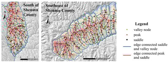
Figure 6.
Results of two areas in aeolian sand dunes to Loess hill and Loess ridge landform.
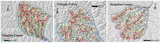
Figure 7.
Results of three areas in Loess hill landform (the legend is the same as that in Figure 6).
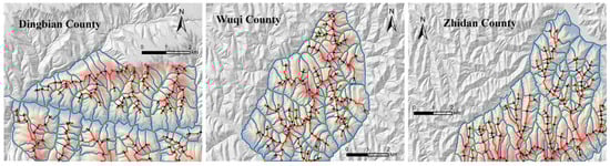
Figure 8.
Results of three areas in Loess ridge landform (the legend is the same as that in Figure 6).
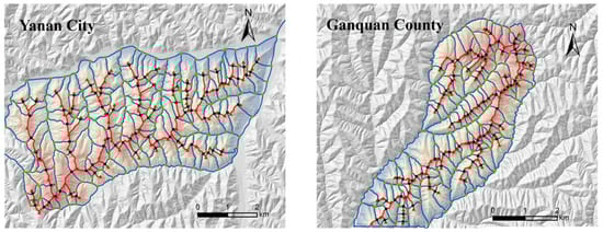
Figure 9.
Results of Yanan City and Ganquan County (the legend is the same as that in Figure 6).
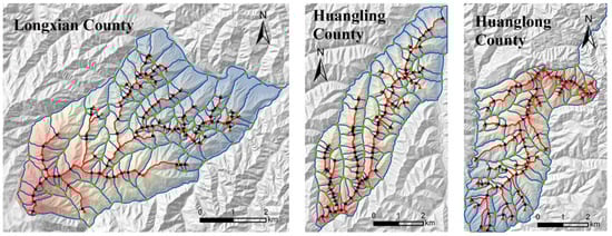
Figure 10.
Results of Longxian County, Huangling County, and Huanglong County (the legend is the same as that in Figure 6).
The terrain skeleton lines in the south of the study area are sparse, and those in the north are dense. The more northerly the sample area is, the more complex the terrain skeleton becomes. Connection lines in the Loess hill are shorter than that in the Loess ridge. The shape of Loess hill, especially Zichang County, is the most complicated, with the highest number of terrain control points. The terrain skeletons of Yanan City and Ganquan County are regular, showing straight valleys and ridges.
3.2. Analysis of the Terrain Skeleton Results
- NNI
Table 2 shows the NNI results of the three types of points and all points combined. Various types of points have different aggregation laws in these landforms. Aeolian sand dunes to Loess hill and Loess ridge in south of Shenmu County have the highest NNI of peaks and saddles, while LLoess-covered middle mountain and intermountain Loess in Longxian County have the lowest. Yanan City located in the junction of Loess hill and Loess-covered middle mountain has the highest NNI of valley nodes. Wuqi County and Dingbian County, which have Loess ridge landform, have the minimum NNIs of valley nodes. When all points are calculated together, Yanan City has the highest NNI, and Long County has the lowest. The point NNIs vary within the same landform area, such as similar NNIs of Loess hill, and the different NNI values of Loess ridge. On the whole study area, there is still a trend of low in the south and high in the north, and low in the west and high in the east (Figure 11). This finding shows that the Loess landform in the northeast of study area is more mature.
Table 2.
NNI results of sample areas.
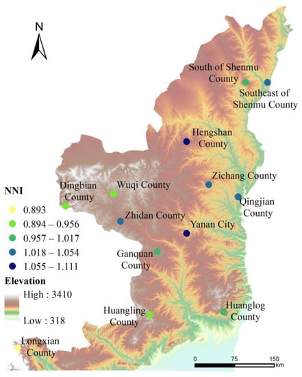
Figure 11.
The spatial distribution of the NNI of the points.
- 2.
- TCI
Table 3 shows the number of edges, number of points, and TCI values of 13 sample regions. The maximum number of edges and points are Loess hill such as Zichang County, Yanan City, and Hengshan County. The sample regions with the same type landform show varying number edges and nodes. Accordingly, the connectivity is not nearly similar, and the numerical interval is inconsistent. Figure 12 shows the distribution of TCI results in the map, which reflects the obvious difference of TCI between regions and the same trend as NNI in the whole study area.
Table 3.
TCI results of sample areas.
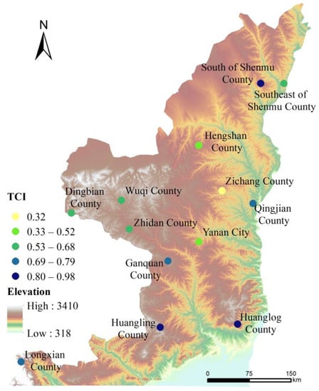
Figure 12.
The spatial distribution map of TCI values in 13 sample areas.
- 3.
- LSI
Table 4 shows the results of the LSI values in 13 sample areas. The value is smallest in the Loess-covered mild middle tableland, Loess-covered moderate relief middle mountain, and Loess-covered middle mountain and intermountain Loess, which are located in the south of the study area. Three sample areas of Loess hill have the maximum LSI. The LSIs of two sample areas, south of Shenmu County and southeast of Shenmu County, vary in the aeolian sand dunes to Loess hill and Loess ridge. In the same landform of Loess ridge, the LSI value of Dingbian County is relatively smaller. The shape of the patch becomes more complex with the increase in LSI. Specifically, the development of Loess hill is the most complicated, followed by Loess ridge, middle mountain, and tableland in the south is the least mature. Figure 13 shows the spatial distribution of the LSI results.
Table 4.
LSI results of sample areas.
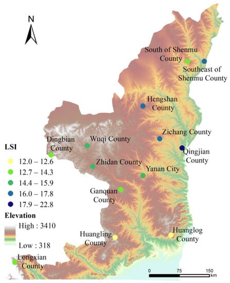
Figure 13.
Spatial distribution of LSI.
The results of the three indicators show obvious regional differences in the topography of the Loess Plateau in northern Shaanxi. However, there are still differences in different areas of the same landform within the landform types classified by Li. The values of two sample areas in Shenmu County are not similar, which belong to aeolian sand dunes to Loess hill and Loess ridge landform. The NNI value of Zhidan County is quite different from Wuqi County and Dingbian County. The TCI value of Qingjian County is much smaller than those of the other two sample areas the in Loess hill landform.
4. Conclusions
The terrain skeleton indicates the presence of significant terrain features. This work realizes a new method of constructing terrain skeleton. The terrain control points needed in the method complete the extraction according to the existing methods. The peaks and saddles are connected by the anti-D8 algorithm, the saddles and valley nodes are connected by the D8 algorithm. Accordingly, an effective connection of the terrain control points are obtained. Lastly, a data structure for the terrain skeleton of this work is designed to better analyze the terrain skeleton. Three indicators were selected related to the three types of geometry of point, line, and surface to describe differences of sample areas with different landforms. The results show that the three selected indicators can reflect the spatial structure of points cluster and describe the landform development to a certain extent. The nearest proximity index can faintly reflect the difference in the aggregation of points in different landforms. The TCI and landscape shape index reflect the characteristics between different landforms.
The boundary of landform type is a process from quantitative change to qualitative change [60]. The various landform types mark the different stages of landform development. The intertwined areas of similarities and differences can be found on both sides of the boundary. The similarity results in the complexity of the boundary of the geomorphic types. Although the quantitative expression of mathematics provides an important theoretical basis for the division of landform types, it is still a complicated scientific problem. The CPB-based division method starts from the data itself and has stable division efficiency and accuracy on the basis of conforming to geographic cognition. However, this CPB-based division method requires manual-inputted initial parameters, and the division process is a black box. The spatial shape, structural characteristics, and quantitative indicators of the terrain skeleton are inherently related to the evolution stage of the landform as a result of long-term evolution. This work is based on the research carried out by this natural law. Time-series terrain data can be used in the future to construct time varying terrain skeleton, establish the corresponding relationship between the quantitative indicators of the terrain skeleton and the landform development stage, and realize the calibration of the landform development stage.
Author Contributions
Conceptualization, Min Li and Ting Wu; methodology, Weitao Li and Chun Wang; software, Xu Su and Yuanyuan Zhao; validation, Wen Dai; formal analysis, Min Li; resources, Weitao Li; data curation, Ting Wu; writing—original draft preparation, Min Li and Ting Wu; writing—review and editing, Min Li and Wen Dai; visualization, Min Li; All authors have read and agreed to the published version of the manuscript.
Funding
This work was financially supported by the Open Project Program of State Key Laboratory of Luminescence and Applications (SKLA-2021-07) and the Natural Science Foundation of China (Nos. 41571398 and 41701450).
Institutional Review Board Statement
Not applicable.
Informed Consent Statement
Not applicable.
Data Availability Statement
Data sharing is not applicable to this article.
Conflicts of Interest
The authors declare no conflict of interest.
References
- Peizhi, H.; Lai, P.-C. The derivation of skeleton lines for terrain features. Geo-Spat. Inf. Sci. 2002, 5, 68–73. [Google Scholar] [CrossRef][Green Version]
- Xiong, L.; Tang, G.; Yang, X.; Li, F. Geomorphology-oriented digital terrain analysis: Progress and perspectives. J. Geog. Sci. 2021, 31, 456–476. [Google Scholar] [CrossRef]
- Li, S.; Hu, G.; Cheng, X.; Xiong, L.; Tang, G.; Strobl, J. Integrating topographic knowledge into deep learning for the void-filling of digital elevation models. Remote Sens. Environ. 2022, 269, 112818. [Google Scholar] [CrossRef]
- Aumann, G.; Ebner, H.; Tang, L. Automatic derivation of skeleton lines from digitized contours. ISPRS J. Photogramm. Remote Sens. 1991, 46, 259–268. [Google Scholar] [CrossRef]
- Podobnikar, T. Production of integrated terrain model from multiple datasets of different quality. Int. J. Geogr. Inf. Sci. 2005, 19, 68–89. [Google Scholar] [CrossRef]
- Thibault, D.; Gold, C.M. Terrain reconstruction from contours by skeleton construction. GeoInformatica 2000, 4, 349–373. [Google Scholar] [CrossRef]
- Gold, C.M.; Dakowicz, M. The Crust and Skeleton–Applications in GIS. In Proceedings of the Second international symposium on Voronoi diagrams in science and engineering, Seoul, Korea, 25 March 2005; pp. 33–42. [Google Scholar]
- Hutchinson, M.F.; Gallant, J.C. Representation of terrain. Geogr. Inf. Syst. 1999, 1, 105–124. [Google Scholar]
- Lv, G.; Xiong, L.; Chen, M.; Tang, G.; Sheng, Y.; Liu, X.; Song, Z.; Lu, Y.; Yu, Z.; Zhang, K. Chinese progress in geomorphometry. J. Geog. Sci. 2017, 27, 1389–1412. [Google Scholar] [CrossRef]
- Bolongaro-Crevenna, A.; Torres-Rodriguez, V.; Sorani, V.; Frame, D.; Ortiz, M.A. Geomorphometric analysis for characterizing landforms in Morelos State, Mexico. Geomorphology 2005, 67, 407–422. [Google Scholar] [CrossRef]
- Xiong, L.Y.; Tang, G.A.; Yan, S.J. Grading extraction method of saddles based on DEM. Sci. Surv. Mapping. 2013, 38, 181–183. [Google Scholar]
- Liu, Z.; Yang, A.; Su, D.; Liu, P. Terrain Features Rapid Extraction of Airborne LiDAR. J. Geod. Geodyn. 2018, 38, 1186–1190. [Google Scholar]
- Zhong, T.; Tang, G.A.; Zhou, Y.; Li, R.; Zhang, W. Method of Extracting Surface Peaks Based on Reverse DEMs. Bull. Surv. Mapp. 2009, 4, 35–37. [Google Scholar]
- Zhang, W.; Tang, G.A.; Tao, Y.; Luo, M.L. An improved method to saddles extraction based on runoff concentration simulation in DEM. Sci. Surv. Mapp. 2011, 36, 158–159. [Google Scholar]
- Guoan, T. Progress of DEM and digital terrain analysis in China. Acta Geogr. Sin. 2014, 69, 1305–1325. [Google Scholar]
- Zhang, Y.; Fan, H.; Li, Y. A Method of Terrain Feature Extraction Based on Contour. Acta Geod. Cartogr. Sin. 2013, 42, 574–580. [Google Scholar]
- Jin, H.; Jingxiang, G. Research on the Algorithm of Extracting Ridge and Valley Lines Using Contour Data. Editor. Board Geomat. Inf. Sci. Wuhan Univ. 2005, 8, 282–286. [Google Scholar]
- Ai, T.H.; Zhu, G.R.; Zhang, G.S. Extraction of Landform Features and Organization of Valley Tree Structure Based on Delaunay Triangulation Model. J. Remote Sens. 2003, 7, 292–298. [Google Scholar]
- Lu, G.; Wang, F.-Q. Skeleton extraction algorithm based on the Delaunay triangulation of contour lines. Eng. Surv. Mapp. 2010, 19, 13–16. [Google Scholar]
- Chen, Y.L.; Liu, D.Y. A New Method for Automatic Extraction of Ridge and Valley Axes from DEM. J. Image Graph. 2001, 6, 1230–1234. [Google Scholar]
- Kong, Y.; Fang, L.; Jiang, Y.; Zhang, Y. A new method of extraction terrain feature lines by morphology. Geomat. Inf. Sci. Wuhan Univ. 2012, 37, 996–999. [Google Scholar] [CrossRef]
- Zhou, Y.; Tang, G.-a.; Zhang, T.; Wang, C. A new method for the derivation of terrain skeleton lines based on wire-like analysis window in grid DEMs. Bull. Surv. Mapp. 2007, 10, 67–69. [Google Scholar]
- Gülgen, F.; Gökgöz, T. Automatic extraction of terrain skeleton lines from digital elevation models. Int. Arch. Photogramm. Remote Sens. Spat. Inf. Sci. 2004, 35, 372–377. [Google Scholar]
- Li, Y.; Yang, B.; Yang, Z. Extraction of ridge lines and valley lines from mountainous lidar fround point cloud. J. Geod. Geodyn. 2013, 33, 111–115. [Google Scholar] [CrossRef]
- Mingliang, L. Research on Terrain Feature Point Cluster Based on DEMs; Chinese Academy of Sciences: Chengdu, China, 2008. [Google Scholar]
- Jenčo, M.; Pacina, J.; Shary, P.A. Terrain skeleton and local morphometric variables: Geosciences and computer vision technique. Adv. Geoinf. Technol. 2009, 57–76. [Google Scholar]
- Zhang, H.J.; Liu, Y.X.; Ma, Z.Q.; He, X.T.; Bao, N. A terrain skeleton feature extraction method based on morphological encoding. J. Comput. Res. Dev. 2015, 52, 1409. [Google Scholar]
- Huang, P. A New Method for Extracting Terrain Feature Lines from Digitized Terrain Data. Ed. Board Geomat. Inf. Sci. Wuhan Univ. 2001, 26, 247–252. [Google Scholar]
- Zhang, H.; Ma, Z.; Liu, Y.; He, X.; Ma, Y. A new skeleton feature extraction method for terrain model using profile recognition and morphological simplification. Math. Prob. Eng. 2013, 2013, 523729. [Google Scholar] [CrossRef]
- Hsu, S. Automatic extraction of ridge and valley axes using the profile recognition and polygon-breaking algorithm. Comput. Geosci. 1998, 24, 83–93. [Google Scholar]
- Liu, Z.-H.; Huang, P.-Z. Derivation of skeleton line from topographic map with DEM data. Sci. Surv. Mapp. 2003, 28, 33–36. [Google Scholar]
- Chen, Y.; Yang, C.; Chen, X.; Sun, Y.; Lin, C. Skeleton line gradation method based on tree structure. J. China Univ. Min. Technol. 2015, 44, 1119–1125. [Google Scholar]
- Zhou, Y.; Tang, G.; Yang, X.; Xiao, C. Positive and negative terrains on northern Shaanxi Loess Plateau. J. Geog. Sci. 2010, 20, 64–76. [Google Scholar] [CrossRef]
- Li, M.; Yang, X.; Na, J.; Liu, K.; Jia, Y.; Xiong, L. Regional topographic classification in the North Shaanxi Loess Plateau based on catchment boundary profiles. Prog. Phys. Geogr. 2017, 41, 302–324. [Google Scholar] [CrossRef]
- Institute of Surveying and Mapping of State Bureau of Surveying and Mapping. Technical Rules for Producing Digital Products of 1:10000 1:50000 Fundamental Geographic Information Part 2: Digital Elevation Models; State Bureau of Surveying and Mapping: Beijing, China, 2007. [Google Scholar]
- Tang, G.; Li, F.; Liu, X. Digital elevation Model Tutorial; Science Press: Nanjing, China, 2010. [Google Scholar]
- Zhong, Y.; Wei, W.; Li, Z.Y. A research on the mathematical definition of the basic landform shape. Sci. Surv. Mapp. 2002, 27, 3. [Google Scholar]
- Fukumura, T.T. Extraction of structural information from grey pictures. Comput. Graph. Image Processing 1978, 7, 30–51. [Google Scholar]
- Chen, P.; Lu, P.; Liu, W.; Song, L. Automatic extraction method of peak point based on self-sealing countour surface. Geospat. Inf. 2020, 18, 4. [Google Scholar]
- Gu, L.; Wang, C.; Li, P.; Wang, J.; Wang, Z. Research on mountain top extraction accuracy based on DEM. Geomat. Inf. Sci. Wuhan Univ. 2016, 41, 131–135. [Google Scholar]
- Gu, L.; Wang, C.; Liu, M.; Yang, Z. A model of extracting surface peak height precision based on DEM. Enineering Surv. Mapp. 2013, 22, 3. [Google Scholar]
- Wood, J.W. The geomorphological characterization of digital elevation models. Ph.D. Dissertation, University of Leicester, Leicester, UK, 1996. [Google Scholar]
- Peucker, T.K.; Douglas, D.H. Detection of Surface-Specific Points by Local Parallel Processing of Discrete Terrain Elevation Data. Comput. Graph. Image Processing 1975, 4, 375–387. [Google Scholar] [CrossRef]
- Kong, Y.; Yi, W.; Zhang, Y. Extracting saddle point fast based on topological relationship. Comput. Eng. Appl. 2013, 49, 165–167. [Google Scholar]
- Huang, N.; Yang, X.; Liu, H. A method of saddle point extraction based on countour spatial relationship. J. Geo-Inf. Sci. 2020, 22, 12. [Google Scholar]
- Wu, T.; Wang, C.; Li, M.; Song, H.; Xu, Y. Terrain saddle point extraction method constrained by morphological features. J. Chuzhou Univ. 2021, 23, 5. [Google Scholar]
- Yi, H.; Tang, G.; Liu, Y.; Yang, X.; Zhu, H. Stream runoff nodes and their derivation based on DEM. J. Soil Water Conserv. 2003, 17, 5. [Google Scholar]
- Zhu, H.; Tang, G.; Wu, L.; Qian, K. Extraction and analysis of gully nodes based on geomorphological structure and catchment characteristics: A case study in the Loess Plateau of north Shaanxi province. Adv. Water Sci. 2012, 23, 7. [Google Scholar]
- Li, J.; Li, T.; Chen, Z.; Liu, X.; Tang, G. Research on channel network nodes based on DEM in hill and gully area of the Loess Plateau. Arid Land Geogr. 2005, 28, 6. [Google Scholar]
- Jiang, L.; Wang, C.; Li, F. Research on elimination method of flat triangle based on ArcGIS. In Proceedings of the Academic Seminar of The Theory and Method Professional Committee of China Geographic Information System Association, Shanghai, China, 28–29 September 2010. [Google Scholar]
- Gong, X.; Shi, H.; Qi, Z. Research on spatial pattern evolution of A-grade tourist attractions in Gansu province. Resour. Dev. Mark. 2017, 33, 219. [Google Scholar]
- Ripley, B.D. Modelling Spatial Patterns. J. R. Stat. Soc. 1977, 39, 172–212. [Google Scholar] [CrossRef]
- Yu, L. Landscape connectivity in soil erosion research: Concepts, implication and quantification. Geogr. Res. 2016, 35, 8. [Google Scholar]
- Yang, Y.; Wang, Y.; Cheng, X.; Li, W.; Gao, M.; Wang, J.; Fu, L.; Zhang, R. Establishment of an ecological security pattern based on connectivity index: A case of the Three Gorges Reservior area in Chongqing. Acta Ecol. Sin. 2020, 40, 13. [Google Scholar]
- Jie, G. Analysis of transportantion network connectivity evaluation index. J. Transp. Eng. Inf. 2010, 1, 35–38. [Google Scholar]
- Xiao, D. Index System and Research Methods of Landscape Spatial Structure; China Forestry Publishing House: Beijing, China, 1991. [Google Scholar]
- Yan, M.; Li, J.; Xiaoyan, K. A extent effect analysis of corelation of landscape indices based on long-temporal series data: A case study of Shijiazhuang City. Geogr. Geo-Inf. Sci. 2021, 31, 79–85. [Google Scholar]
- Bin, L.; Jintun, Z. The Shape Indices and Scale Fractal Analysis of Shrub Landscape in the Loess Plateau. Chin. Agric. Sci. Bull. 2009, 5. [Google Scholar]
- Canran, L.; Lingzhi, C. Analysis of the patch shape with shape indices for the vegetation landscape in Beijing. Acta Ecol. Sin. 2000, 20, 559–567. [Google Scholar]
- Li, S.; Xiong, L.; Tang, G.; Strobl, J. Deep learning-based approach for landform classification from integrated data sources of digital elevation model and imagery. Geomorphology 2020, 354, 107045. [Google Scholar] [CrossRef]


Publisher’s Note: MDPI stays neutral with regard to jurisdictional claims in published maps and institutional affiliations. |
© 2022 by the authors. Licensee MDPI, Basel, Switzerland. This article is an open access article distributed under the terms and conditions of the Creative Commons Attribution (CC BY) license (https://creativecommons.org/licenses/by/4.0/).