
A Vector Field Approach to Estimating Environmental Exposure Using Human Activity Data


Abstract
:1. Introduction
2. Related Work
2.1. Spatial Justice
2.2. Environmental Exposure
2.3. Vector Field
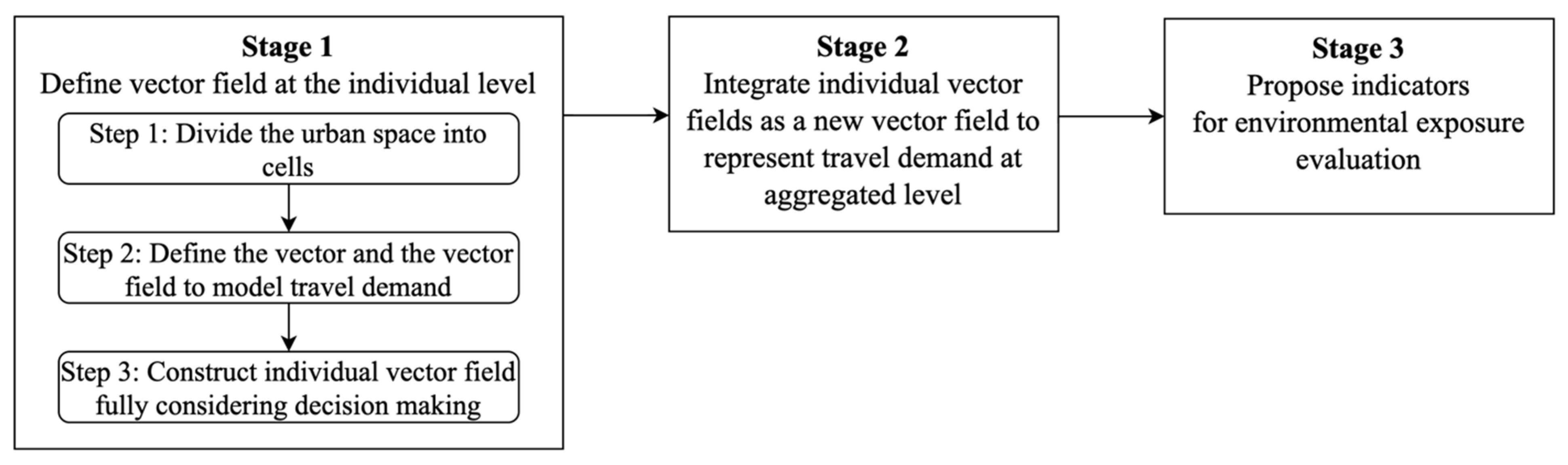
3. Methodology
3.1. Vector Field at the Individual Level
3.1.1. Divide the Urban Space into Cells
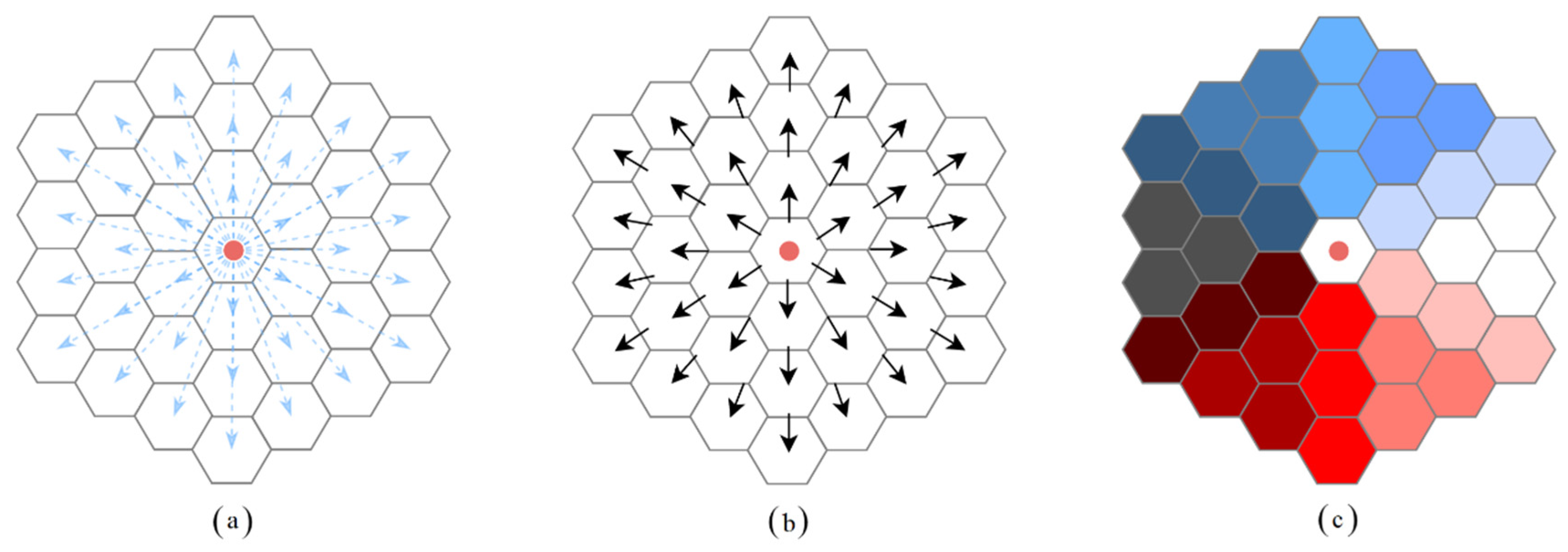
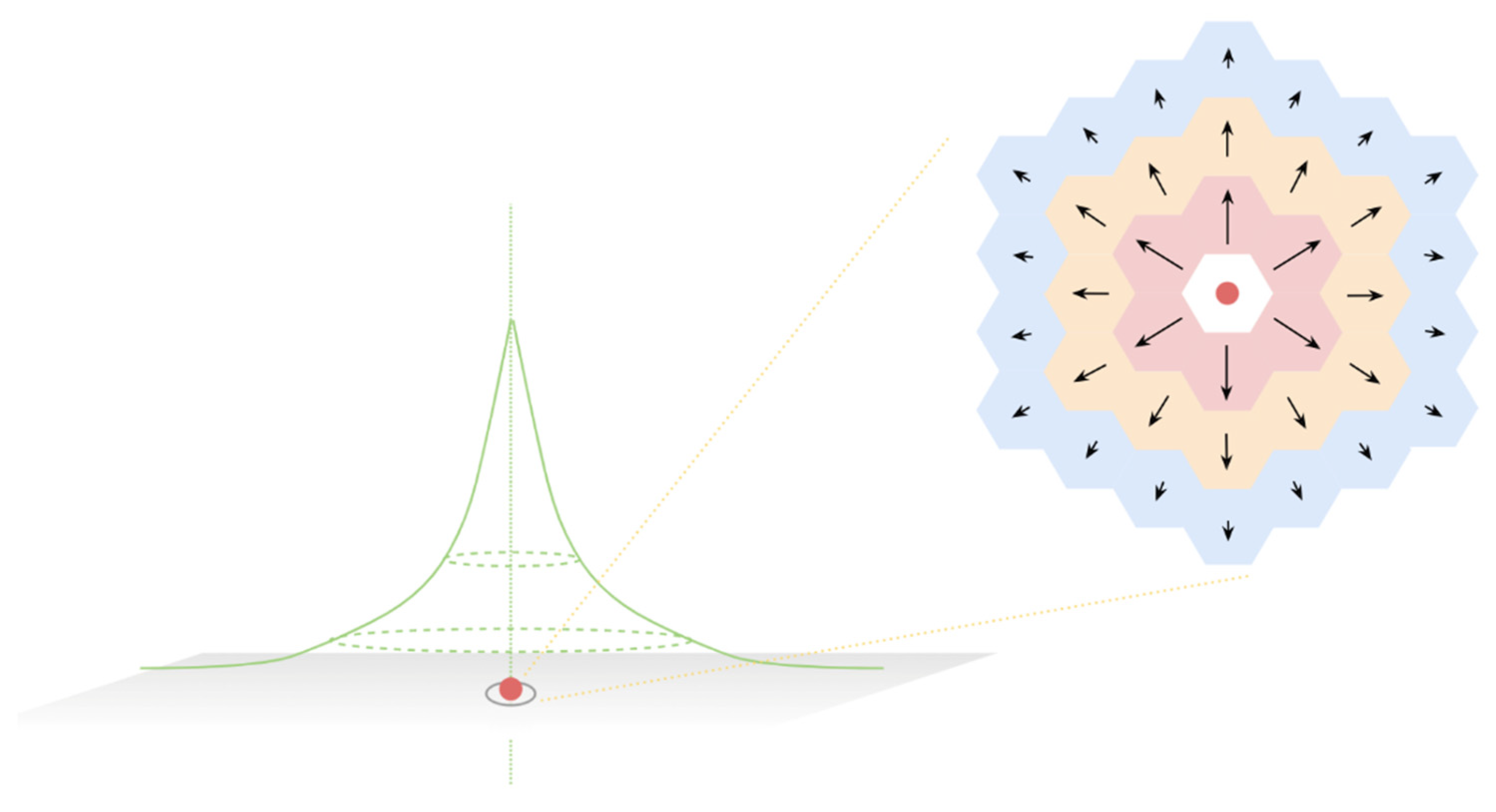
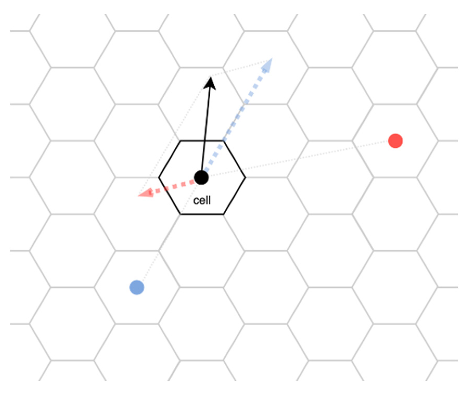
3.1.2. Define the Vector and the Vector Field
3.1.3. Create the Vector Field at the Individual Level
| Algorithm 1: Build vector field for individuals |
| 1: initialize sum_vector; //an indexed data structure with id as the index 2: for each activity point api in ap_list do 3: ap_lati ← api’s latitude; 4: ap_loni ← api’s longitude; 5: for each centroid point cpj in cp_list do 6: cp_latj ← cpj ’s latitude; 7: cp_lonj ← cpj ’s longitude; 8: idj ← cpj ’s point ID; 9: distanceij, angleij ← inverse solution for the geodesic (ap_lati, ap_loni, cp_latj, cp_lonj); 10: moduleij ← e ^ (−0.167 * distanceij −3.575); 11: vectorij ←vector packaging (moduleij, angleij); 12: sum_vector(idj) ←sum_vector(idj)+vectorij; //using vector addition 13: merge sum_vector and cp_list by point’s ID id to get output(id); 14: final; 15: return output; |
3.2. Travel Demand at the Population Level
| Algorithm 2: Build travel demand vector field for population (or specific groups) |
| 1: initialize output; //an indexed data structure with id as the index 2: for each point’s ID idi in id_list do 3: for each individual vector field vfj in vf_list do 4: vectorij ←vfj (idi)’s vector; //fetching vector at that position 5: moduleij ←vectorij ’s module; 6: output(idi) ←output(idi)+moduleij; //using scalar addition 7: final; 8: return output; |
3.3. Environmental Exposure Evaluation
4. Case Study
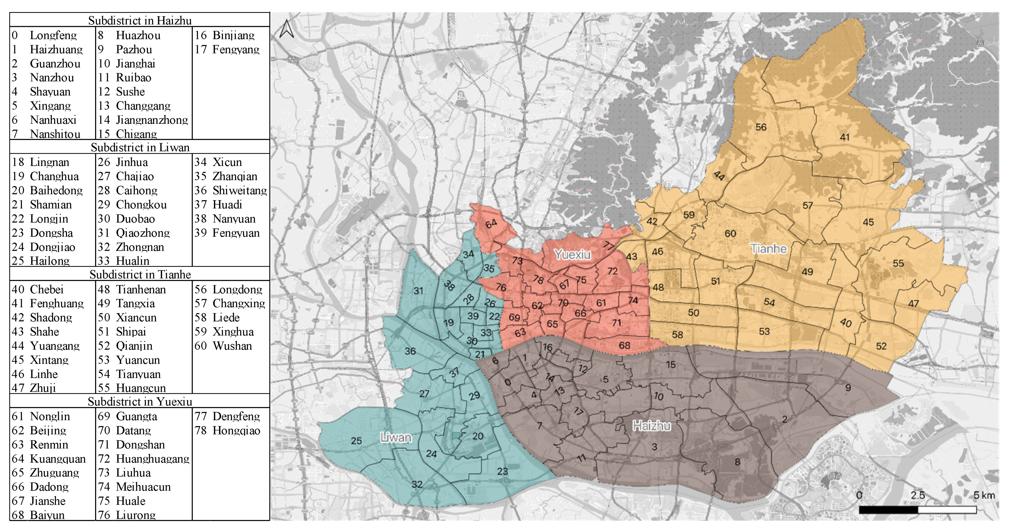
4.1. Study Area
4.2. Dataset and Data Processing
4.2.1. Daily Mobility Survey
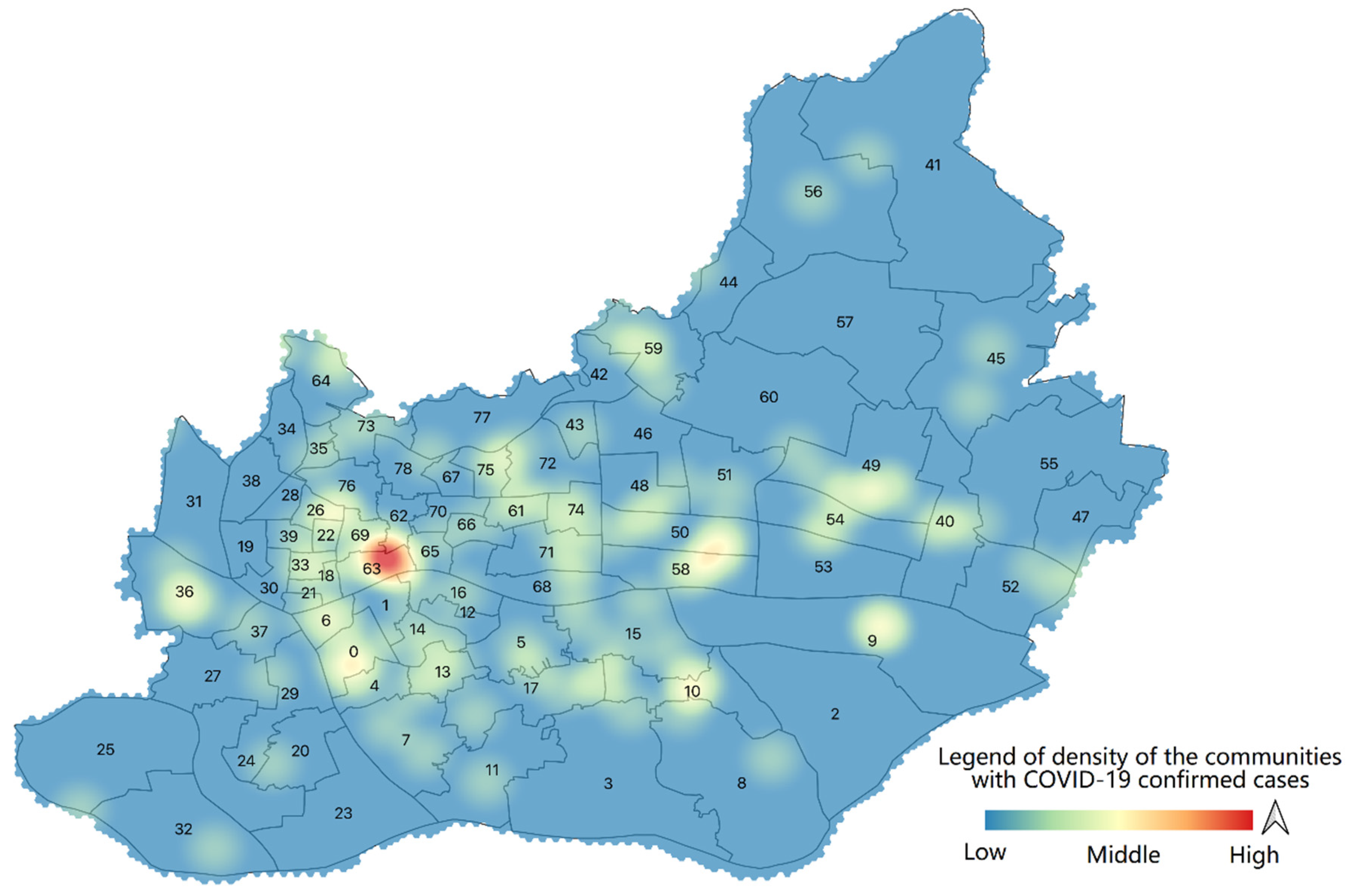
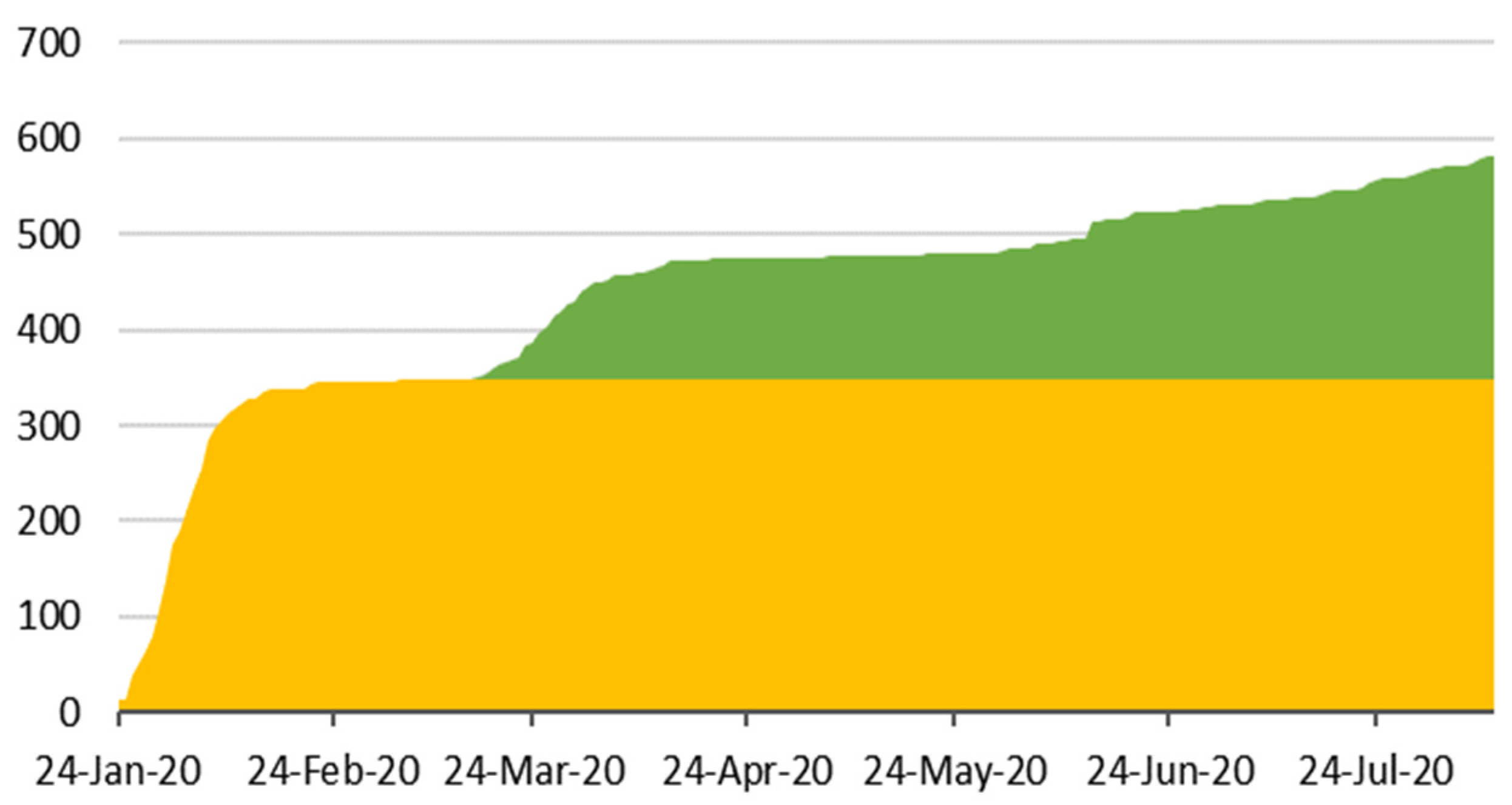
4.2.2. COVID-19 Reports
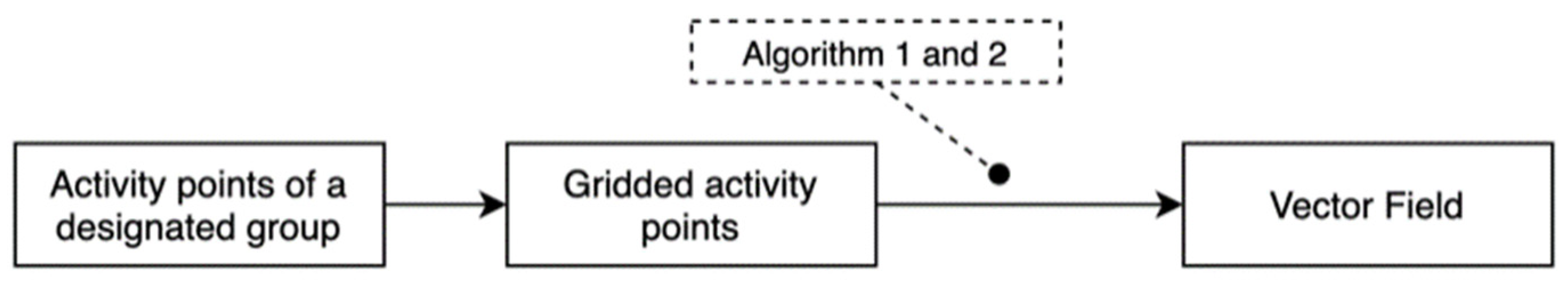
4.3. Constructing Vector Field to Model Travel Demand
4.4. Calculating the Groups’ Pandemic Exposure
5. Result
5.1. Travel Demand of Each Social Group
5.2. Pandemic Exposure Evaluation and Comparison for Various Demographic Groups
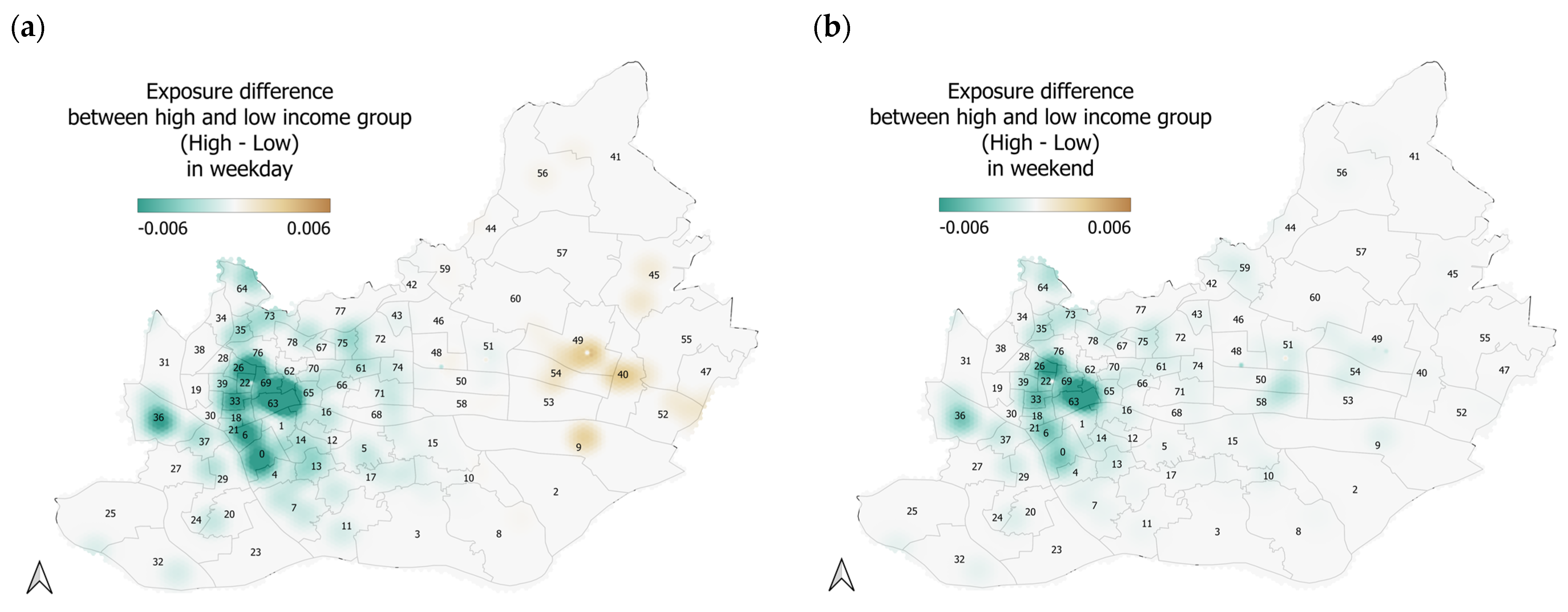
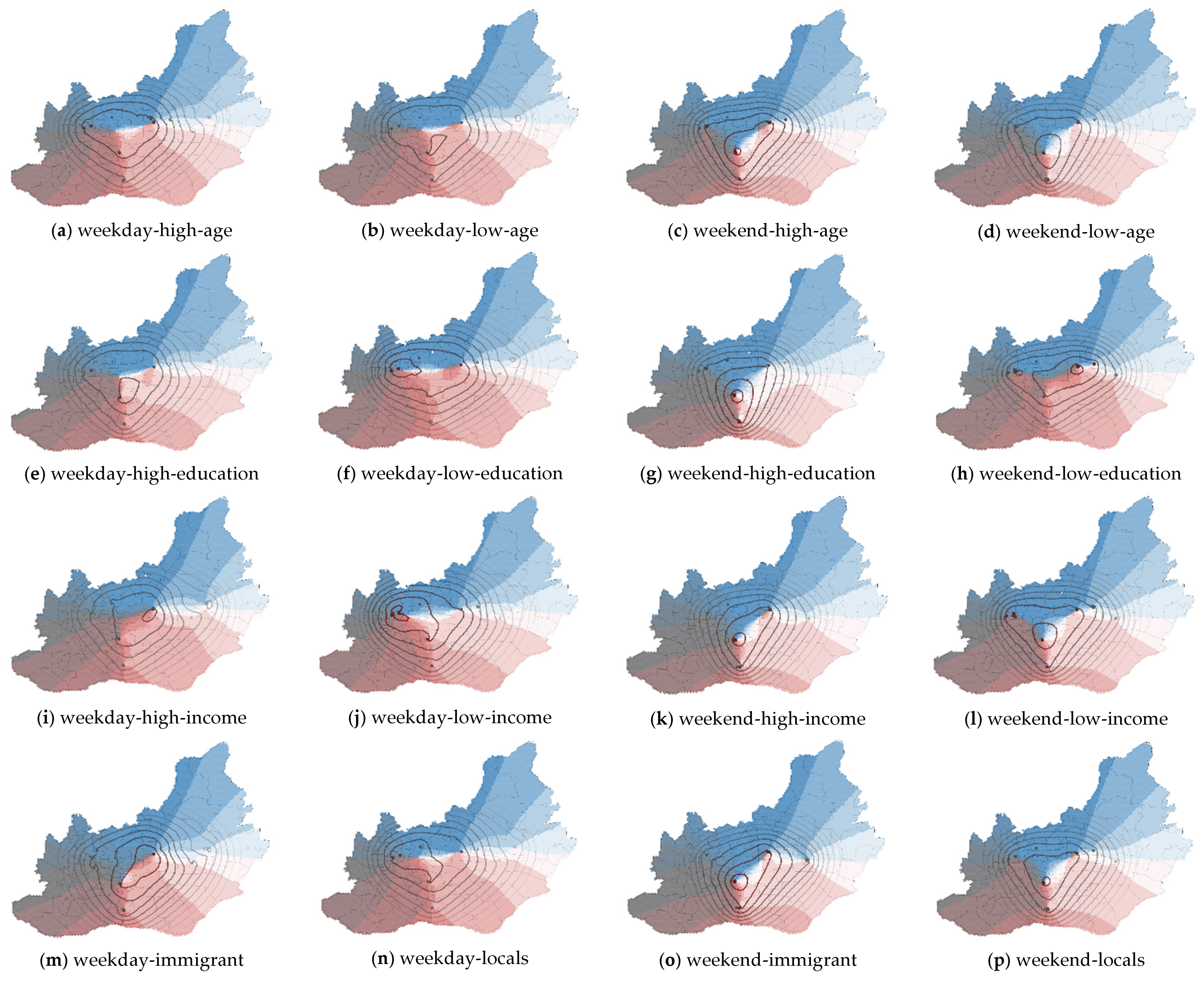
5.3. Pandemic Exposure Evaluation and Comparison in Space
6. Discussion and Conclusions
Author Contributions
Funding
Data Availability Statement
Conflicts of Interest
References
- Braun-Fahrländer, C.; Riedler, J.; Herz, U.; Eder, W.; Waser, M.; Grize, L.; Maisch, S.; Carr, D.; Gerlach, F.; Bufe, A.; et al. Environmental exposure to endotoxin and its relation to asthma in school-age children. N. Engl. J. Med. 2002, 347, 869–877. [Google Scholar] [CrossRef] [PubMed] [Green Version]
- Satarug, S.; Garrett, S.H.; Sens, M.A.; Sens, D.A. Cadmium, environmental exposure, and health outcomes. Environ. Health Perspect. 2010, 118, 182–190. [Google Scholar] [CrossRef]
- Templeton, A.; Guven, S.T.; Hoerst, C.; Vestergren, S.; Davidson, L.; Ballentyne, S.; Madsen, H.; Choudhury, S. Inequalities and identity processes in crises: Recommendations for facilitating safe response to the COVID-19 pandemic. Br. J. Soc. Psychol. 2020, 59, 674–685. [Google Scholar] [CrossRef] [PubMed]
- Redondo-Sama, G.; Matulic, V.; Munté-Pascual, A.; de Vicente, I. Social work during the COVID-19 crisis: Responding to urgent social needs. Sustainability 2020, 12, 8595. [Google Scholar] [CrossRef]
- Soja, E. The city and spatial justice. Spat. Justice 2009, 1, 1–5. [Google Scholar]
- Wiesner, M.R.; Lowry, G.V.; Jones, K.L.; Hochella, M.F., Jr.; Di Giulio, R.T.; Casman, E.; Bernhardt, E.S. Decreasing uncertainties in assessing environmental exposure, risk, and ecological implications of nanomaterials. Environ. Sci. Technol. 2009, 43, 6458–6462. [Google Scholar] [CrossRef] [Green Version]
- Zhang, L.; Zhou, S.; Kwan, M.P.; Chen, F.; Lin, R. Impacts of individual daily greenspace exposure on health based on individual activity space and structural equation modeling. Int. J. Environ. Res. Public Health 2018, 15, 2323. [Google Scholar] [CrossRef] [Green Version]
- Kwan, M.-P.; Wang, J.; Tyburski, M.; Epstein, D.H.; Kowalczyk, W.J.; Preston, K.L. Uncertainties in the geographic context of health behaviors: A study of substance users’ exposure to psychosocial stress using GPS data. Int. J. Geogr. Inf. Sci. 2019, 33, 1176–1195. [Google Scholar] [CrossRef]
- Coccia, M. An index to quantify environmental risk of exposure to future epidemics of the COVID-19 and similar viral agents: Theory and practice. Environ. Res. 2020, 191, 110155. [Google Scholar] [CrossRef]
- Rodes, C.E.; Kamens, R.M.; Wiener, R.W. The significance and characteristics of the personal activity cloud on exposure assessment measurements for indoor contaminants. Indoor Air 1991, 1, 123–145. [Google Scholar] [CrossRef]
- Su, J.G.; Morello-Frosch, R.; Jesdale, B.M.; Kyle, A.D.; Shamasunder, B.; Jerrett, M. An index for assessing demographic inequalities in cumulative environmental hazards with application to Los Angeles, California. Environ. Sci. Technol. 2009, 43, 7626–7634. [Google Scholar] [CrossRef] [PubMed] [Green Version]
- Padilla, C.M.; Kihal-Talantikite, W.; Vieira, V.M.; Rossello, P.; Le Nir, G.; Zmirou-Navier, D.; Deguen, S. Air quality and social deprivation in four French metropolitan areas—A localized spatio-temporal environmental inequality analysis. Environ. Res. 2014, 134, 315–324. [Google Scholar] [CrossRef] [PubMed] [Green Version]
- Milojevic, A.; Niedzwiedz, C.L.; Pearce, J.; Milner, J.; MacKenzie, I.A.; Doherty, R.M.; Wilkinson, P. Socioeconomic and urban-rural differentials in exposure to air pollution and mortality burden in England. Environ. Health 2017, 16, 104. [Google Scholar] [CrossRef] [Green Version]
- Yang, N.; Fu, R.; Chao, Y.; Liu, H.; Ma, X. Quantitative assessment of environmental exposure of delivery men in Wuhan. Arch. Environ. Occup. Health 2020, 75, 445–463. [Google Scholar] [CrossRef] [PubMed]
- Miller, H.J.; Bridwell, S.A. A field-based theory for time geography. Ann. Assoc. Am. Geogr. 2009, 99, 49–75. [Google Scholar] [CrossRef]
- Liu, X.; Yan, W.Y.; Chow, J.Y.J. Time-geographic relationships between vector fields of activity patterns and transport systems. J. Transp. Geogr. 2015, 42, 22–33. [Google Scholar] [CrossRef]
- Liu, X.; Chow JY, J.; Li, S. Online monitoring of local taxi travel momentum and congestion effects using projections of taxi GPS-based vector fields. J. Geogr. Syst. 2018, 20, 253–274. [Google Scholar] [CrossRef] [Green Version]
- McAloon, C.; Collins, Á.; Hunt, K.; Barber, A.; Byrne, A.W.; Butler, F.; Casey, M.; Griffin, J.; Lane, E.; McEvoy, D.; et al. Incubation period of COVID-19: A rapid systematic review and meta-analysis of observational research. BMJ Open 2020, 10, e039652. [Google Scholar] [CrossRef]
- Tang, B.; Xia, F.; Tang, S.; Bragazzi, N.L.; Li, Q.; Sun, X.; Liang, J.; Xiao, Y.; Wu, J. The effectiveness of quarantine and isolation determine the trend of the COVID-19 epidemics in the final phase of the current outbreak in China. Int. J. Infect. Dis. 2020, 95, 288–293. [Google Scholar] [CrossRef]
- Goldthorpe, J.H. Sociology as a Population Science; Cambridge University Press: Cambridge, UK, 2016. [Google Scholar]
- Gross, C.P.; Essien, U.R.; Pasha, S.; Gross, J.R.; Wang, S.Y.; Nunez-Smith, M. Racial and ethnic disparities in population-level Covid-19 mortality. J. Gen. Intern. Med. 2020, 35, 3097–3099. [Google Scholar] [CrossRef]
- Cwalina, S.N.; Ihenacho, U.; Barker, J.; Smiley, S.L.; Pentz, M.A.; Wipfli, H. Advancing racial equity and social justice for Black communities in US tobacco control policy. Tob. Control 2021. [Google Scholar] [CrossRef] [PubMed]
- Jian, I.Y.; Luo, J.; Chan, E.H. Spatial justice in public open space planning: Accessibility and inclusivity. Habitat Int. 2020, 97, 102122. [Google Scholar] [CrossRef]
- Liu, X.; Lin, Z.; Huang, J.; Gao, H.; Shi, W. Evaluating the Inequality of Medical Service Accessibility Using Smart Card Data. Int. J. Environ. Res. Public Health 2021, 18, 2711. [Google Scholar] [CrossRef] [PubMed]
- Chan, C.S.; Shek, K.F. Are Guangdong-Hong Kong-Macao Bay area cities attractive to university students in Hong Kong? Leading the potential human capital from image perception to locational decisions. J. Place Manag. Dev. 2021, 14, 404–429. [Google Scholar] [CrossRef]
- Ayeb-Karlsson, S.; Kniveton, D.; Cannon, T. Trapped in the prison of the mind: Notions of climate-induced (im) mobility decision-making and wellbeing from an urban informal settlement in Bangladesh. Palgrave Commun. 2020, 6, 62. [Google Scholar] [CrossRef] [Green Version]
- Xie, Y.; Danaf, M.; Azevedo, C.L.; Akkinepally, A.P.; Atasoy, B.; Jeong, K.; Seshadri, R.; Ben-Akiva, M. Behavioral modeling of on-demand mobility services: General framework and application to sustainable travel incentives. Transportation 2019, 46, 2017–2039. [Google Scholar] [CrossRef]
- Oldenkamp, R.; Hoeks, S.; Čengić, M.; Barbarossa, V.; Burns, E.E.; Boxall, A.B.; Ragas, A.M. A high-resolution spatial model to predict exposure to pharmaceuticals in European surface waters: EPiE. Environ. Sci. Technol. 2018, 52, 12494–12503. [Google Scholar] [CrossRef]
- Xu, Y.; Jiang, S.; Li, R.; Zhang, J.; Zhao, J.; Abbar, S.; González, M.C. Unraveling environmental justice in ambient PM2.5 exposure in Beijing: A big data approach. Comput. Environ. Urban Syst. 2019, 75, 12–21. [Google Scholar] [CrossRef]
- Song, Y.; Chen, B.; Kwan, M.P. How does urban expansion impact people’s exposure to green environments? A comparative study of 290 Chinese cities. J. Clean. Prod. 2020, 246, 119018. [Google Scholar] [CrossRef]
- Huang, J.; Kwan, M.P. Uncertainties in the assessment of COVID-19 risk: A Study of people’s exposure to high-risk environments using individual-level activity data. Ann. Am. Assoc. Geogr. 2021, 1–20. [Google Scholar] [CrossRef]
- Cartaxo, A.N.S.; Barbosa, F.I.C.; de Souza Bermejo, P.H.; Moreira, M.F.; Prata, D.N. The exposure risk to COVID-19 in most affected countries: A vulnerability assessment model. PLoS ONE 2021, 16, e0248075. [Google Scholar] [CrossRef] [PubMed]
- Kulu, H.; Dorey, P.S. Infection rates from Covid-19 in Great Britain by geographical units: A model-based estimation from mortality data. Health Place 2021, 67, 102460. [Google Scholar] [CrossRef] [PubMed]
- Elson, R.; Davies, T.M.; Lake, I.R.; Vivancos, R.; Blomquist, P.B.; Charlett, A.; Dabrera, G. The spatio-temporal distribution of COVID-19 infection in England between January and June 2020. Epidemiol. Infect. 2021, 149, 1–19. [Google Scholar] [CrossRef] [PubMed]
- Selander, J.; Nilsson, M.E.; Bluhm, G.; Rosenlund, M.; Lindqvist, M.; Nise, G.; Pershagen, G. Long-term exposure to road traffic noise and myocardial infarction. Epidemiology 2009, 20, 272–279. [Google Scholar] [CrossRef] [PubMed]
- Wang, M.; Aaron, C.P.; Madrigano, J.; Hoffman, E.A.; Angelini, E.; Yang, J.; Laine, A.; Vetterli, T.M.; Kinney, P.L.; Sampson, P.D.; et al. Association between long-term exposure to ambient air pollution and change in quantitatively assessed emphysema and lung function. JAMA 2019, 322, 546–556. [Google Scholar] [CrossRef]
- Larsen, K.; Black, P.; Rydz, E.; Nicol, A.M.; Peters, C.E. Using geographic information systems to estimate potential pesticide exposure at the population level in Canada. Environ. Res. 2020, 191, 110100. [Google Scholar] [CrossRef] [PubMed]
- Morrison, C.N.; Byrnes, H.F.; Miller, B.A.; Kaner, E.; Wiehe, S.E.; Ponicki, W.R.; Wiebe, D.J. Assessing individuals’ exposure to environmental conditions using residence-based measures, activity location-based measures, and activity path-based measures. Epidemiology 2019, 30, 166. [Google Scholar] [CrossRef]
- Wang, J.; Kwan, M.P.; Chai, Y. An innovative context-based crystal-growth activity space method for environmental exposure assessment: A study using GIS and GPS trajectory data collected in Chicago. Int. J. Environ. Res. Public Health 2018, 15, 703. [Google Scholar] [CrossRef] [Green Version]
- Zhao, P.; Liu, X.; Shi, W.; Jia, T.; Li, W.; Chen, M. An empirical study on the intra-urban goods movement patterns using logistics big data. Int. J. Geogr. Inf. Sci. 2020, 34, 1089–1116. [Google Scholar] [CrossRef]
- Torres Ochaita, Á. Betados/Vector_2d. GitHub. 2018. Available online: https://github.com/betados/vector_2d (accessed on 26 April 2020).
- Blundell, R.; Costa Dias, M.; Joyce, R.; Xu, X. COVID-19 and Inequalities. Fiscal Studies 2020, 41, 291–319. [Google Scholar] [CrossRef]
- Che, L.; Du, H.; Chan, K.W. Unequal pain: A sketch of the impact of the COVID-19 pandemic on migrants’ employment in China. Eurasian Geogr. Econ. 2020, 61, 448–463. [Google Scholar] [CrossRef]
- Millett, G.A.; Jones, A.T.; Benkeser, D.; Baral, S.; Mercer, L.; Beyrer, C.; Honermann, B.; Lankiewicz, E.; Mena, L.; Crowley, J.S. Assessing differential impacts of COVID-19 on black communities. Ann. Epidemiol. 2020, 47, 37–44. [Google Scholar] [CrossRef] [PubMed]
- Kwan, M.-P. The uncertain geographic context problem. Ann. Assoc. Am. Geogr. 2012, 102, 958–968. [Google Scholar] [CrossRef]
- Zhao, P.; Kwan, M.P.; Zhou, S. The uncertain geographic context problem in the analysis of the relationships between obesity and the built environment in Guangzhou. Int. J. Environ. Res. Public Health 2018, 15, 308. [Google Scholar] [CrossRef] [Green Version]
- Tuan, Y.F. Space and Place: The Perspective of Experience; University of Minnesota Press: Minneapolis, MN, USA, 1977. [Google Scholar]
- Guangzhou Municipal Health Commission. Guangzhou Municipal Health Commission Website-Epidemic Notification. Guangzhou Municipal Health Commission. Available online: http://wjw.gz.gov.cn/ztzl/xxfyyqfk/yqtb/index.html (accessed on 10 March 2021).
- Thakar, V. Unfolding events in space and time: Geospatial insights into COVID-19 diffusion in Washington State during the initial stage of the outbreak. ISPRS Int. J. Geo-Inf. 2020, 9, 382. [Google Scholar] [CrossRef]
- Lbs.Amap.Com. AMap Geocoding/Reverse Geocoding API Documentation. Available online: https://lbs.amap.com/api/webservice/guide/api/georegeo (accessed on 11 August 2020).
- Geopandas Developers. Geopandas/Geopandas: v0.8.1. Zenodo. 2020. Available online: https://zenodo.org/record/3946761#.YgeXjpaxVhF (accessed on 11 August 2020).
- Toms, S. ArcPy and ArcGIS–Geospatial Analysis with Python; Packt Publishing Ltd.: Birmingham, UK, 2015. [Google Scholar]
- Gdal/Ogr Contributors. GDAL/OGR Geospatial Data Abstraction Software Library; Open Source Geospatial Foundation: Beaverton, OR, USA, 2021. [Google Scholar]
- Lee, H.; Miller, V.J. The disproportionate impact of COVID-19 on minority groups: A social justice concern. J. Gerontol. Soc. Work. 2020, 63, 580–584. [Google Scholar] [CrossRef]


| ID | Start Time | End Time | Latitude | Longitude | Place Change |
|---|---|---|---|---|---|
| 1001-01-1 | 3:00:00 | 7:00:00 | 23.127996 | 113.25522 | 1 |
| 1001-01-2 | 7:00:00 | 7:15:00 | 23.127996 | 113.25522 | 3 |
| 1001-01-3 | 7:15:00 | 7:30:00 | 23.127996 | 113.25522 | 4 |
| 1001-01-4 | 7:30:00 | 8:00:00 | 23.127996 | 113.25522 | 3 |
| Name | TEI | Name | TEI | ||
|---|---|---|---|---|---|
| Weekday-high-income | 3.59 | 1.67 | Weekend-high-income | 3.49 | 1.19 |
| Weekday-low-income | 3.94 | 1.79 | Weekend-low-income | 3.77 | 1.35 |
| Weekday-high-age | 3.81 | 1.77 | Weekend-high-age | 3.78 | 1.35 |
| Weekday-low-age | 3.71 | 1.68 | Weekend-low-age | 3.48 | 1.19 |
| Weekday-high-education | 3.69 | 2.20 | Weekend-high-education | 3.61 | 1.60 |
| Weekday-low-education | 3.89 | 1.25 | Weekend-low-education | 3.68 | 0.94 |
| Weekday-migrant | 3.83 | 0.83 | Weekend-migrant | 3.71 | 0.65 |
| Weekday-local | 3.74 | 2.62 | Weekend-local | 3.61 | 1.89 |
| Rank | Name | ID | Weekday-High-Income | Weekday-Low-Income | Weekend-High-Income | Weekend-Low-Income | ||||
|---|---|---|---|---|---|---|---|---|---|---|
| TEI | TEI | TEI | TEI | |||||||
| 1 | Renmin | 63 | 36.97 | 17.23 | 46.24 | 20.95 | 37.23 | 12.73 | 43.27 | 15.45 |
| 2 | Guangta | 69 | 27.28 | 12.71 | 34.69 | 15.72 | 27.01 | 9.24 | 32.25 | 11.51 |
| 3 | Longjin | 22 | 19.64 | 9.15 | 25.06 | 11.35 | 18.34 | 6.27 | 22.56 | 8.05 |
| … | … | … | … | … | … | … | … | … | … | … |
| 77 | Guanzhou | 2 | 0.05 | 0.02 | 0.05 | 0.02 | 0.05 | 0.02 | 0.05 | 0.02 |
| 78 | Dongsha | 23 | 0.01 | 0.00 | 0.01 | 0.01 | 0.01 | 0.003 | 0.01 | 0.004 |
| 79 | Changxing | 57 | 0.00 | 0.00 | 0.00 | 0.00 | 0.00 | 0.00 | 0.00 | 0.00 |
Publisher’s Note: MDPI stays neutral with regard to jurisdictional claims in published maps and institutional affiliations. |
© 2022 by the authors. Licensee MDPI, Basel, Switzerland. This article is an open access article distributed under the terms and conditions of the Creative Commons Attribution (CC BY) license (https://creativecommons.org/licenses/by/4.0/).
Share and Cite
Guo, Z.; Liu, X.; Zhao, P. A Vector Field Approach to Estimating Environmental Exposure Using Human Activity Data. ISPRS Int. J. Geo-Inf. 2022, 11, 135. https://doi.org/10.3390/ijgi11020135
Guo Z, Liu X, Zhao P. A Vector Field Approach to Estimating Environmental Exposure Using Human Activity Data. ISPRS International Journal of Geo-Information. 2022; 11(2):135. https://doi.org/10.3390/ijgi11020135
Chicago/Turabian StyleGuo, Zijian, Xintao Liu, and Pengxiang Zhao. 2022. "A Vector Field Approach to Estimating Environmental Exposure Using Human Activity Data" ISPRS International Journal of Geo-Information 11, no. 2: 135. https://doi.org/10.3390/ijgi11020135
APA StyleGuo, Z., Liu, X., & Zhao, P. (2022). A Vector Field Approach to Estimating Environmental Exposure Using Human Activity Data. ISPRS International Journal of Geo-Information, 11(2), 135. https://doi.org/10.3390/ijgi11020135