Analysis of Urban Vitality in Nanjing Based on a Plot Boundary-Based Neural Network Weighted Regression Model

Abstract

As a representative indicator for the level and sustainability of urban development, urban vitality has been widely used to assess the quality of urban development. However, urban vitality is too blurry to be accurately quantified and is often limited to a particular type of expression of vitality. Current regression models often fail to accurately express the spatial heterogeneity of vibrancy and drivers. Therefore, this paper took Nanjing as the study area and quantified the social, cultural, and economic vitality indicators based on mobile phone data, POI data, and night-light remote sensing data. We also mapped the spatial distribution of comprehensive urban vitality using an improved entropy method and analyzed the spatial heterogeneity of urban vitality and its influencing factors using a plot boundary-based neural network weighted regression (PBNNWR). The results show: (1) The comprehensive vitality in Nanjing is distributed in a “three-center” pattern with one large and two small centers; (2) PBNNWR can be used to investigate the local regression relationships among the driving factors and urban vitality, and the fitting accuracy (95.6%) of comprehensive vitality in weekdays is higher than that of ordinary least squares regression (OLS) (65.9%), geographically weighted regression (GWR) (89.9%), and geographic neural network weighted regression (GNNWR) (89.5%) models; (3) House price, functional diversity, building density, metro station accessibility, and residential facility density are factors that significantly affect urban vitality. The study’s findings can provide theoretical guidance for optimizing the urban spatial layout, resource allocation, and targeted planning strategies for areas with different vitality values.

1. Introduction

The overwhelming process of urbanization and global population growth has led to a surge in the number of urban dwellers from 751 million in 1950 to 4.2 billion in 2018, and the management of urban areas has become one of the most critical development challenges facing the world in the 21st century [1]. Rapid urbanization has been accompanied by urban sprawl and irrational planning, which has reduced the ecological quality of affected regions [2] and even led to the emergence of empty cities and ghost towns in many places [3]. The excessive pursuit of faster urbanization and neglect of people-centered growth have seriously affected residents’ quality of life [4,5]. Therefore, a comprehensive assessment of the development quality of cities is needed to provide theoretical guidance for the optimization of urban spatial layout and resource allocation. As an indicator of urban attractiveness, cohesiveness, and ability to support various social activities [6], increased urban vitality can provide a positive emotional and psychological experience for citizens [7] and enhance the sustainability of socio-economic development. Therefore, assessing urban vitality and proposing targeted vitality creation strategies would serve to mitigate the problems associated with rapid urbanization and promote quality urban development.

Previous research on urban vitality has focused on the concept of urban vitality, quantitative analysis of urban vitality, and investigation of the influencing factors of urban vitality. The concept of urban vitality often varies according to the concerns of researchers. From the perspective of urban morphology, urban vitality is regarded as a product of spatial morphological design [8]. Jacobs was the representative who focused more on the microscopic expression of urban vitality, and she argued that urban vitality comes from people and their activities in space and proposed four characteristics of a vibrant city: a mix of land functions, small block sizes, diversity of building eras, and concentration of population [9]. Subsequently, Lynch, Montgomery, and Gehl refined the definition of urban vitality at the microform design level [6,10,11].

From the theory of urban economics, some studies argue that urban vitality is an essential engine for the economy of the country in which it is located, and identify dynamism as economic and technological competitiveness from a macro perspective [12]. In the development of urban economy, an urbanized economy with a concentration of competitive firms generates positive externalities to the local area, to a certain extent. Mature financial security policies and technological conditions can attract external capital and highly qualified labor, which provide stable impetuses for the growth of urban economic dynamism. Therefore, in these studies, the most dynamic cities tend to gather a large number of competitive firms and have the ability to bring in capital and attract external populations [13,14]. In addition, some researches divide urban vitality into social, economic, and cultural vitality from an urban sociological perspective [15]. Such studies measure the ability of cities to develop and survive on their own at a macro level, as well as the degree of support for various daily activities of inhabitants [16,17].

The quantitative assessment of urban vitality can help to objectively investigate urban development [18], and finding a scientific and effective method is the key to quantifying urban vitality. In the early stages of research, scholars mainly used questionnaires and statistical yearbooks to calculate vitality values [19]. Although the results obtained from the questionnaire data were accurate, they were more costly and time-consuming. As the statistics were mostly static and not fine scale, the study area was often limited by small size or coarse scale. With the development of communication and remote sensing technologies, Baidu heat maps [20], night-light remote sensing images [21], mobile phone data [22,23], and social media check-in data [24,25] are becoming increasingly available. These datasets can help researchers to study urban vitality from the overall structure to see clear differences by providing extensive, objective, and real-time observations [26,27,28]. Tu et al. [26] used POI density, mobile phone record density, and check-in density as proxies for urban vitality and then derived urban vitality according to the entropy weight method. Wang and Liu et al. [28] used mobile phone check-in data and POI data to obtain urban vitality values from the perspective of consumer activity density and diversity in each community. However, when using multiple sources of big data, there is an overlap of different data. For instance, the population density recorded by mobile phones and social check-in density both describe human behavior, which may shift the focus of the vibrancy quantification results toward population activity intensity.

Therefore, according to urban sociology theory, it is possible to quantify the comprehensive urban vitality from the perspective of society, economy, and culture using corresponding data [15]. Social vitality is closely related to the activities and mobility of urban residents, and is commonly measured by social media data, taxi track data, and mobile phone data. Due to its strong privacy, wide distribution, and high temporal resolution, mobile phone data can effectively express spatiotemporal changes in urban social vitality [29]. Economic vitality demonstrates the capacity and potential of a city in the process of economic development [12]. Traditional macro study data suffer from low resolution and missing areas, so fine-grained data such as Dianping, house price, and night-time light brightness are commonly used to characterize economic vitality [25]. Compared with Dianping data, which rely on user reviews and are challenging to obtain, and house price data, which are highly volatile and unevenly distributed, night light remote sensing data have characteristics of simple access and spatially rich detail, and are a good indicator of economic vitality at neighborhood and grid scales [30,31]. Cultural vitality reflects the occurrence of cultural activities in a city. It can be quantified by the number of cultural POIs, library collections, people engaged in cultural activities and students per unit of population, output of cultural industries, and input of cultural resources [19,32]. Cultural POIs are widely used to measure urban cultural vitality due to their rich semantics, high accuracy, and easy accessibility.

Exploring influencing factors of urban vitality can help suggest targeted vibrancy creation, which is essential to optimize the efficiency of urban construction and urban development decisions [33]. The qualities of favorable built environments, street design, and proper distribution of facilities are catalysts for improving residential quality and promoting the healthy development of the region [34], which have also been shown to create more vibrant urban spaces [35]. Indicators such as block size, road network density, building density, land use intensity, land use mix, and spatial accessibility [24,36,37,38,39,40], and models such as linear regression methods [41], geographically weighted regression (GWR) [24,27], Geodetector [42], and other non-linear regression models that take the spatial heterogeneity of geographic factors into account have been used to explore the various driving factors of urban vitality. Liu and Zhang et al. [22] chose mobile phone data as a proxy for urban vitality, and designed ten indicators such as POI density, land use mix, building density, and wage level as vitality drivers. They used the GWR model to investigate the regression relationship between urban social vitality, economic vitality, and the drivers. Fang et al. [7] used the spatial design network analysis technique to quantify 16 indicators of street density, connectivity, and separation, and established the relationship between urban vitality values and the above indicators by Geodetector. Urban vitality shows complex and variable spatial heterogeneity owing to the influence of the built environment and land function. However, the GWR model has shortcomings in exploring spatial non-stationarity relationships due to its simple structure of the weight kernel function [43]. To overcome the impact of spatial heterogeneity of associated factors, Du et al. [44] used a geographically neural network weighted regression model (GNNWR) to analyze the relationship between factors such as temperature, precipitation, and atmospheric PM2.5 concentrations. The results found that by modifying the kernel function, GNNWR could fit the effect of spatiotemporal proximity on weights, which possessed higher fitting accuracy than the GWR model. In addition, GNNWR accurately reflected the differences in the fluctuation of the relationship between geographical factors across different geographical locations.

The emergence of the sociology of urban vitality has brought comprehensiveness and objectivity to quantifying urban vitality. At the same time, the GNNWR provides a new perspective for analyzing the relationship between influencing factors and urban vitality. This study took Nanjing as the study area and used the improved entropy weight method to obtain the spatial structure of comprehensive urban vitality from social, economic, and cultural aspects. To address the shortcomings of the current regression models, which can only deal with low complexity and spatial heterogeneity between urban vitality and influencing factors, we also proposed a plot boundary-based neural network weighted regression (PBNNWR). It revealed possible factors influencing the structure of Nanjing city vitality.

2. Study Area and Datasets

2.1. Study Area

Nanjing is located in the lower reaches of the Yangtze River in eastern China, with a total area of 6587 km², including 868 km² of built-up area, and 11 districts with a total resident population of 9.31 million (Figure 1). As the only megacity in the Yangtze River Delta, the city is second only to Shanghai in size. With an urbanization rate of 85.2%, well-developed urban infrastructure, and commerce, the city has a dense population and diverse urban functions. In recent years, Nanjing has achieved rapid social and economic development, ranking first among Chinese provincial capitals in terms of GDP per capita in 2020. Nanjing is classified as Beta-level in the ranking of world cities compiled by the Globalization and World Cities Research Network (GaWC), the same rank as Athens and Seattle [45]. In addition, Nanjing was the first Chinese city to be selected by UNESCO as a “World Capital of Literature” and has rich scientific, educational, and cultural resources. Therefore, different types of urban vitality can be fully reflected in the area. According to the Nanjing Urban Plan (2018–2035), the government aims to build a vibrant city that is innovation-driven with international influence and green development. Therefore, Nanjing is perhaps one of the best representatives for studying the vitality and drivers of large cities in the context of China’s urban development, given the combination of current urban development and government policies.

2.2. Data

2.2.1. Mobile Subscriber Data

Mobile phone data was used to characterize social vitality for its ability to provide a detailed picture of the activity and mobility of the population in social activities [42]. The mobile subscriber data was purchased from Jiangsu mobile company, acquired from 18–24 February 2019, covering nine administrative districts in Nanjing (Figure 1c), with a temporal resolution of 0.5 h and a spatial resolution of 150 m. When a user entered the coverage area of a base station, any actions of the mobile phone (e.g., talking, sending and receiving messages, connecting to the network, etc.) were automatically recorded by the base station, and signaling data containing the location and number of the base station were generated. The mobile phone signaling data used in this study were obtained by counting the number of mobile phone users in each base station coverage area every half hour and interpolating the population data into a 150 × 150 m grid. Each grid datum includes the administrative area, time (as shown in

Table 1. The format of mobile subscriber data.

Region	Time	ID	Longitude	Latitude	Age	Num
Jian Ye	201902180230	wtsqjy5	118.728838	32.027868	26–35	116
Jian Ye	201902181430	wtsqjb0	118.724725	32.994904	55+	15

, 20,190,218 for 18 February 2019 and 0230 for half-past two), grid ID, latitude, longitude, and the number of people in each age group of the population. The age information was obtained based on the identity information tied to each user’s mobile phone number. In this paper, we treated Monday (18 February 2019) to Friday (22 February 2019 ) as weekdays and Saturday (23 February 2019) and Sunday (24 February 2019 ) as weekends based on the timestamp, and calculated the sum of the people in all the different age groups to get the total population of the grid.

2.2.2. POI Data

The POI data for Nanjing were obtained from Gaode (http://map.amap.com/, accessed on 14 December 2022) in December 2018, and each piece of data contained information, such as the name, latitude and longitude, primary category, secondary category, etc. The original data had 19 primary categories and 400 secondary categories, such as company enterprise, life service, tourism service, etc. According to the Map of Essential Urban Land Use Categories (EULUC) classification system [46], the data were reclassified into nine categories: residential, business, commercial, industrial, government institutions, education, medical, cultural, and public services. It was necessary to reconstruct the different types of POIs because of their uneven distribution in terms of number and space, mainly including: (1) deleting POIs of commercial type with a distance less than 10 m; (2) overlaying POIs and Google images to add public service POIs through visual interpretation; and (3) using random forest method to supplement industrial and residential POIs. The specific details of the reconstruction and spatial distribution of POIs before and after the reconstruction can be found in the literature [47,48]. Through the reconstruction of POIs, the problems of significant differences in the number of different types of POIs and the sparse distribution of POIs around the suburb of the city have been improved. We chose cultural POIs to characterize cultural vitality and used the number of different types of POIs to calculate the land use mix index.

2.2.3. Night-Time Lighting Data

It has been shown that there is a positive correlation between light brightness and economic vitality [30]. The night-time light data was downloaded from the official website of Luojia-1 (http://59.175.109.173:8888/index.html, accessed on 14 December 2022), and images with no clouds and high imaging quality acquired on 27 September 2018 were selected. The latitude and longitude of the image center are 118.689773 and 31.796713, respectively. We used night-time light remote sensing images to calculate the study area’s economic vitality.

2.2.4. OSM Data

The OSM data were obtained from the OpenStreetMap website (https://www.openstreetmap.org, accessed on 14 December 2022), downloaded in December 2018, and includes vector data of roads, railways, and water bodies. There are seven types of roads, namely primary road, secondary road, tertiary road, residential road, motorway, trunk, and railway, which were used to delineate the traffic analysis area of this paper.

2.2.5. Traffic Analysis Area (TAZ)

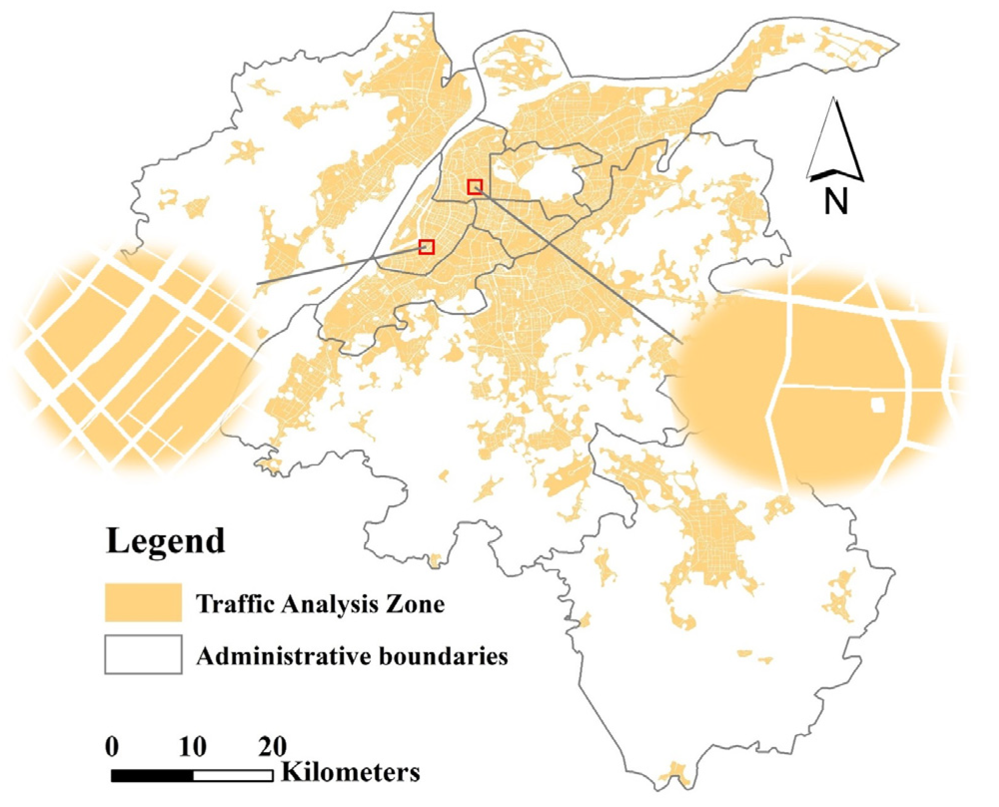
The traffic analysis area in Nanjing was obtained by overlaying the OSM road network and impervious surface data, which characterizes the extent of the built-up urban area. Impervious surface refers to artificial ground surfaces such as roofs or asphalt or concrete pavements that cannot be permeated by water, and we downloaded free impervious surface maps (GAIA) with up to 90% accuracy from the Tsinghua website (http://data.ess.tsinghua.edu.cn/, accessed on 14 December 2022) [49]. The main methods for generating TAZ [48] are as follows: (1) Gather statistical distribution of the road widths at each level in the OSM and obtain the corresponding widths as the radius of the road buffers with the rule of choosing the upper quartile for primary roads, and the median for secondary roads, e.g., 44 m for primary roads, 34.8 m for secondary roads, etc.; (2) Overlay seven levels of road buffers with the impervious surface distribution map of the study area to obtain a total of 8209 TAZs; (3) Remove fine TAZs that are not suitable for human activities (e.g., flowerbeds in the middle of the road) through visual interpretation. We obtained 5513 TAZs (parcels) (Figure 2), with a minimum area of 4600 m² and a maximum area of 120,000 m². This paper chose TAZs as the basic unit for urban vitality analysis.

2.2.6. Other Datasets

The following datasets were used to calculate the driving variables of urban vitality.

(1)

Building data

The building vector data of the study area was downloaded from the BIGEMAP platform (http://www.bigemap.com/, accessed on 14 December 2022), including contour polygons and heights. For locations in the suburbs where buildings were missing, we supplied them with visual interpretation by overlaying with Google Earth high-resolution remote sensing images. Building heights were obtained by the inversion of the shadow lengths of images [48], resulting in 163,840 building profile vector data for Nanjing.

(2)

House price data

The listing data for the study area were crawled in Python from the Lianjia platform (https://nj.lianjia.com/, accessed on 14 December 2022) in December 2021. The data contain information both on rental and second-hand housing listings. There were 48,352 rental listings and 101,634 second-hand listings, all containing title, total price, unit price, area, latitude, and longitude. As the data had some redundancy and coordinate offset, data cleaning was carried out to (1) remove non-housing data, such as garages and basements; (2) convert housing coordinates from the BD-09 coordinate system to the WGS-84 coordinate system; (3) transfer housing points appearing on roads to the interior of buildings by visual interpretation according to maps and housing descriptions; and (4) obtain second-hand housing price data by interpolating rental data for the missing data areas.

(3)

Sentinel-2 data

The 1C-level Sentinel-2 remote sensing images for the whole year of 2018 were acquired from the ESA Copernicus Data Centre (https://scihub.copernicus.eu, accessed on 14 December 2022). After pre-processing, such as atmospheric correction and resampling, the NDVI value of each image element was calculated, and the 2018 synthetic image was generated with the maximum NDVI image element values for the whole year [48].

(4)

Subway station data

Nanjing metro station data was crawled from Gaode Map (http://map.amap.com/, accessed on 14 December 2022) for 2019, with 174 stations covering 10 lines.

3. Method

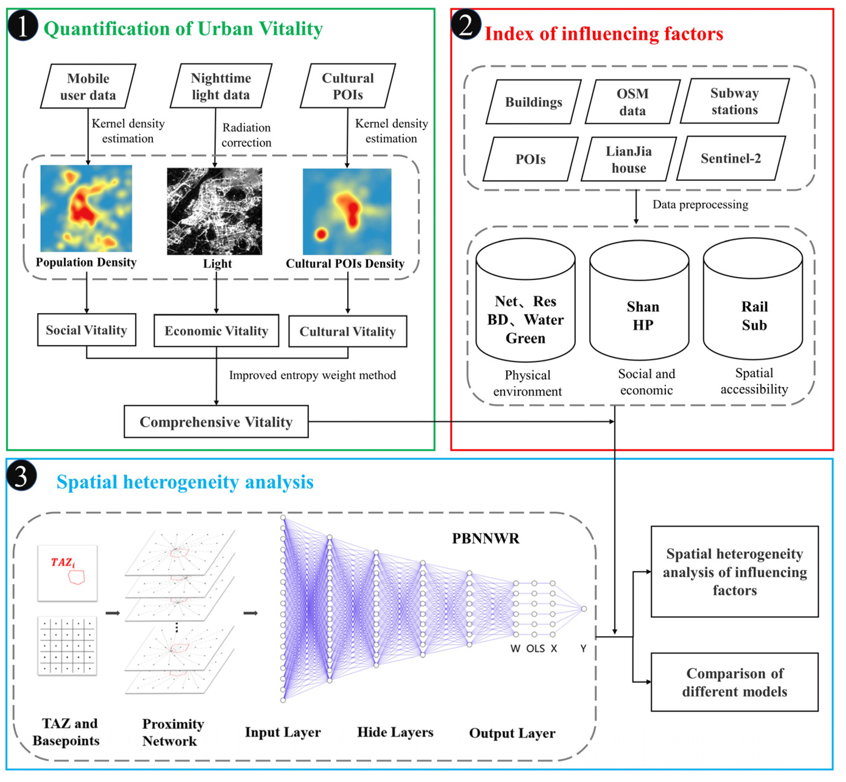
This paper divides the research methodology into the following three parts (Figure 3): (1) Quantifying the urban cultural, economic, and social vitality using Gaode POI, night-time light remote sensing imagery, and mobile phone data, respectively, and then calculating comprehensive urban vitality value using an improved entropy method; (2) Constructing an index system in terms of the physical environment, socio-economy, and spatial accessibility indicators using multisource geographic big data; (3) Exploring the drivers of spatial heterogeneity of urban vitality using plot boundary-based neural network weighted regression (PBNNWR) and comparing the simulation results with that of least squares regression (OLS), geographic weighted regression (GWR), and geographic neural network weighted regression (GNNWR).

3.1. Quantification of Urban Vitality

3.1.1. Social Vitality

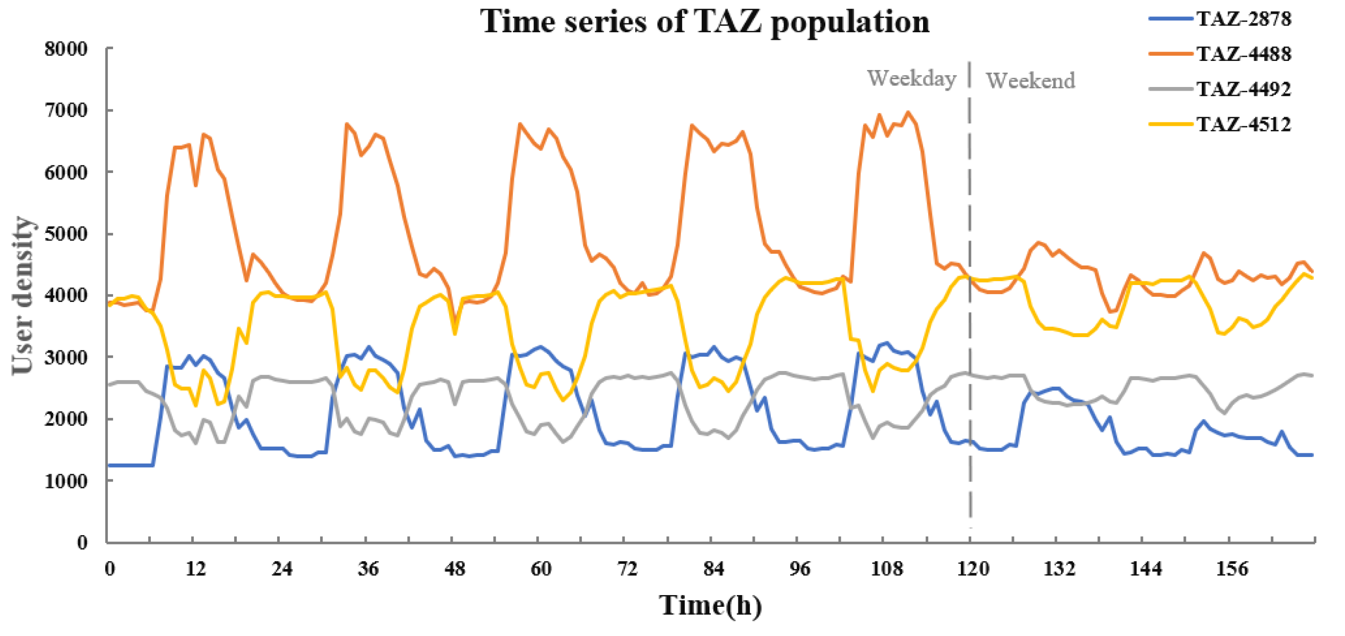
The population aggregation value from the mobile phone data was first used to obtain 168 time periods of 7 days with one-hour intervals. Then, we calculated the sum of the population in each age group as the total population of the grid using the grid ID as the unique identifier, and 168 kernel density maps were drawn using the vector point data. The change curve of mobile phone subscribers of each TAZ in Nanjing was plotted based on the TAZ statistics (Figure 4). By removing anomalous fluctuations in the data, a total of 160 time periods were obtained for this paper.

From the change curves of user density of the four randomly selected TAZs in Figure 4, there is evident periodicity in the change in population density of the TAZs, with differences between weekdays and weekends. Therefore, the average population density of the parcels was separately calculated for weekdays and weekends to obtain the social vitality of the TAZs.

3.1.2. Economic Vitality

We first performed radiation calibration on the Luojia-1 image to convert the image grey-scale values into light brightness values. Then, we performed pan correction against the Google Earth image of Nanjing. Finally, we counted the average brightness of each TAZ and selected the normalized brightness value as the economic vitality. The formula for radiation calibration is as follows:

$$L=D{N}^{\frac{3}{2}}\times {10}^{-10}$$

(1)

where $L$ indicates the light brightness value after radiation correction and $DN$ is the image gray value.

3.1.3. Cultural Vitality

Cultural vitality reflects the activity of cultural events in the city. Cultural facilities provide the necessary space for the generation of cultural activities and cultural vitality; therefore, they can be expressed by the density of cultural POIs [50]. Cultural POIs in Nanjing include media institutions, exhibition centers, galleries, museums, science and technology museums, etc. In this paper, we verified the accuracy of POI distributions via visual interpretation from the Gaode map and then obtained cultural vitality value at each TAZ unit by kernel density analysis, TAZ aggregation, and normalization.

3.1.4. The Change in Urban Vitality

In order to explore the discrepancy in urban vitality between weekdays and weekends, all vitality values were normalized according to the maximum and minimum values on weekdays. Then, the difference in vitality values was calculated.

3.2. Calculation of Comprehensive Urban Vitality by Improving Entropy Method

Single-source big data only measures one aspect of vitality [26]. For example, mobile phone user data are often used to characterize human activity, whereas POI data are applied to describe spatial vitality with quantitative information about facilities. Hence, it is necessary to synthesize the three types of vitality to obtain comprehensive urban vitality [51]. Common methods include the mean method [42], entropy method [52], F-1 score method [28], and factor analysis method [21]. The entropy method uses the property of entropy quantifying the discrete degree of data and finds the degree of difference between different indicators based on the data itself to determine the weights. The method avoids the interference of human factors on the index weight and has strong objectivity of comprehensive evaluation [53].

However, in the case of extreme vitality values, huge data deviation can produce unreasonable weights [54]. In order to improve the instability of the entropy method, we filtered out the neighboring TAZs of each TAZ based on distance and then performed the local entropy method for each TAZ. The obtained indicator weights were only applied to this TAZ. Distance weighting was applied to each datum to weaken the influence of spatial autocorrelation in calculating local weight. The method is as follows:

(1)

Construct the original matrix $X$, where each column denotes a different vitality indicator (population, culture, and economy), each row represents a different sample (i.e., TAZ), and $X_{ij}$ denotes the jth indicator value of sample $i$.

(2)

Taking $TA{Z}_i$ as an example, calculate the centroid distance $D_i$ from other TAZs.

(3)

Use the maximum distance (5000 m) between adjacent TAZs as the search radius, and filter $t$ adjacent TAZs within the search radius to obtain the data matrix:

$$Data\_i={\left[X_1,\dots ,X_t\right]}^T=\left[\begin{array}{ccc}{X}_{11}& \dots & X_{1n}\\ ⋮& \ddots & ⋮\\ X_{t1}& \dots & X_{tn}\end{array}\right]$$

(2)

(4)

For the data of each adjacent TAZ, use distance weighting to attenuate the effect of adjacent TAZs on their vitality, which is calculated as follows:

$$X_s{}^{\prime }=\frac{X_s\ast d_{is}{}^2}{{{\displaystyle \sum }}_{s=1}^t{d}_{is}{}^2}$$

(3)

where $X_s$ and $X_s^{\prime }$ are row vectors indicating the value of each indicator of TAZs before and after weighting, respectively. The distance-weighted dataset was only obtained and used to calculate the weights, with the dataset represented as:

$$temp\_Data\_i={\left[X_1{}^{\prime },\dots ,X_t{}^{\prime }\right]}^T=\left[\begin{array}{ccc}{X}_{11}{}^{\prime }& \dots & X_{1n}{}^{\prime }\\ ⋮& \ddots & ⋮\\ X_{t1}{}^{\prime }& \dots & X_{tn}{}^{\prime }\end{array}\right]$$

(4)

(5)

Perform entropy method operations on the dataset $temp\_Data\_i$, including data normalization, entropy value calculation, difference coefficient calculation, and indicator weight calculation [55], to obtain $n$ indicator weights $W_i$ of $TA{Z}_i$.

(6)

Use the original data $X_i$ and weight values $W_i$ of $TA{Z}_i$ to calculate the comprehensive urban vitality $V_i$:

$$V_i={{\displaystyle \sum }}_{j=1}^n{W}_{ij}\ast X_{ij}$$

(5)

(7)

Repeat steps (2) to (6) to finally obtain the comprehensive vitality value V for all the TAZs in the study area.

3.3. Construction of the Influencing Factors Index of Urban Vitality

3.3.1. Principle of Indicator Construction

The influencing factor indicators of urban vitality can be constructed from three aspects: the physical environment, socio-economics, and spatial accessibility [40]. The physical environment is the foundation of urban vitality, including streets, roads, buildings, and other aspects. Dense road networks [26] and open space facilities can sufficiently meet people’s travel and living needs. A larger building area can carry more people and gather more functions [56], and a good natural environment (e.g., green space and water bodies) helps people to soothe their mood, reduce stress, and promote the generation of various communication activities. We selected road network density, density of residential facilities, building density, green space coverage, and hydrophilicity as physical environment indicators.

Socio-economics is an essential indicator for urban development. Land use mix [22] can ensure the complementarity of urban functions and promote socio-economic growth by improving the efficiency of urban space use. The distribution of house prices can, to a certain extent, reflect the degree of development and economical distribution of the study area. We calculated the diversity of land use and house prices as socio-economic indicators using reclassified POIs and Lianjia house listing data.

Spatial accessibility includes the accessibility of spatial locations such as subway stations and railways. Well-structured and evenly distributed subway stations can help residents reduce commuting costs, and areas with dense stations not only represent higher pedestrian flows but also have a robust radiating effect on the surrounding areas. The vacuum formed around railways due to hazards is usually not conducive to human activities and negatively impacts urban vitality in general [18]. In this paper, the accessibility of subway stations and railways were chosen as spatial accessibility indicators.

3.3.2. Calculation of Influencing Factor Indicators

Data such as OSM, POI, building vectors, house prices, Sentinel-2 images, Google Earth images, and subway stations were used to calculate nine influencing factor indicators in three dimensions. The calculation method is shown in

Table 2. Calculation methods of influencing indicators.

Dimension	Indicator	Calculation Method
Physical environment	Road network density (Net)	The ratio of the total length of the road network within the buffer zone to the buffer zone area. The buffer radius is the average of the minimum spacing of the TAZs.
	Residential density (Res)	The ratio of the number of residential facilities in the TAZ area.
	Building density (BD)	The ratio of the total building area (the number of floors multiplies individual floor area) to the TAZ area.
	Green cover (Green)	The ratio of the total vegetation area to the TAZ buffer area. The vegetation was extracted by visual interpretation and supplied with Google Earth images.
	Hydrophilicity (Water)	Indicated by $D-NEARW\_di{s}_i$. D (500 m) is the search radius of the proximity analysis based on the idea of a 15-min living circle for residents [57], and $NEARW\_di{s}_i$ indicates the distance from the TAZ to the nearest water body.
Socio-economics	Land function diversity (Shan)	Indicated by the Shannon entropy of POI: $Sha{n}_i=-{\displaystyle \sum }_{j=1}^n{p}_{ij}\ast In(p_{ij})$$. n$ denotes the number of POI species within the TAZ and $p_{ij}$ denotes the ratio of the number of the $jth$ POI species to the total number of POIs within the TAZ.
	House prices (HP)	The average value of all the housing unit prices within the TAZ.
Spatial accessibility	Accessibility of subway stations (Sub)	$\mathrm{Indicated}\mathrm{by}K-NEARS\_di{s}_i$$.NEARS\_di{s}_i$ represents the distance from the TAZ to the nearest subway station and $K$ is a constant that is calculated by the average minimum distance between each subway station.
	Rail accessibility (Rail)	$\mathrm{Indicated}\mathrm{by}D-NEARR\_di{s}_i$. The calculation method is the same as that of hydrophilicity.

.

The variance inflation factor (VIF) (Equation (6)) was used to conduct the multiple cointegration test of the independent variables [51]. $R_i^2$ indicates the goodness of fit of the multiple linear regression model with indicator $i$ as the dependent variable and other indicators as independent variables. If $VI{F}_i$ is greater than 7.5, it means serious co-linearity between the independent variables, and this indicator needs to be removed.

$$VI{F}_i=\frac{1}{1-R_i^2}$$

(6)

3.4. PBNNWR Model

In order to detect the driving factors of urban vitality, it is often necessary to make use of various regression models. Global regression models represented by OLS require parameters with spatial stationarity, whereas the spatial heterogeneity inherent in urban vitality cannot meet the requirements of OLS modeling [58]. GWR shows better performance than OLS regression in terms of local spatial variation. However, GWR can only portray simple non-linear relationships [44] and cannot cope with the complex spatial non-stationarity characteristics between urban dynamics and its influencing factors. The GNNWR model, on the other hand, can adequately fit complex non-linear regression relationships between geographic elements but does not consider the varying TAZ sizes and the nonuniformity of spatial distribution. Therefore, we created a PBNNWR model for solving the above spatial heterogeneity problems.

3.4.1. Model Construction

According to the formula of the weight kernel function in GWR:

$$W\left(u_i,v_i\right)=Diag\left(W_1\left(u_i,v_i\right),W_2\left(u_i,v_i\right),\dots ,W_m\left(u_i,v_i\right)\right)$$

(7)

The function $W_j\left(u_i,v_i\right)$, which relied on the spatial distance $d_{ij}$ and bandwidth $h$, can be abstracted as $f\left(d_{ij},h\right)$ and the final weight matrix is obtained:

$$W\left(u_i,v_i\right)=Diag\left(f\left(d_{i1},h\right),f\left(d_{i2},h\right),\dots , f\left(d_{im},h\right)\right)$$

(8)

The accuracy of the regression model is closely related to the sample proximity relationship. Therefore, Du and Wang et al. [44] regarded the spatial non-stationary nature of the regression relationship as the difference in the fluctuation of the spatial relationship to the mean relationship arising from different geographical locations. They used the OLS regression results to represent the mean relationship between geographical elements to create GNNWR, mathematically expressed as:

$$y_i=w_0\left(u_i,v_i\right)\ast {\beta }_{0,OLS}+{{\displaystyle \sum }}_{t=1}^m{w}_t\left(u_i,v_i\right)*{\beta }_{t,OLS}*x_{it}+{\epsilon }_i$$

(9)

The fit matrix can be expressed as:

$${\widehat{Y}}_i=X_i^{T}W\left(u_i,v_i\right){\left(X^{T}X\right)}^{-1}{X}^{T}Y$$

(10)

where $W\left(u_i,v_i\right)$ was solved using a spatial weighted neural network (SWNN), denoted as $W\left(u_i,v_i\right)=SWNN\left(d_{i1},d_{i2},\dots ,d_{im}\right)$, with $d_{ij}$ denoting the Euclidean distance of the sample points.

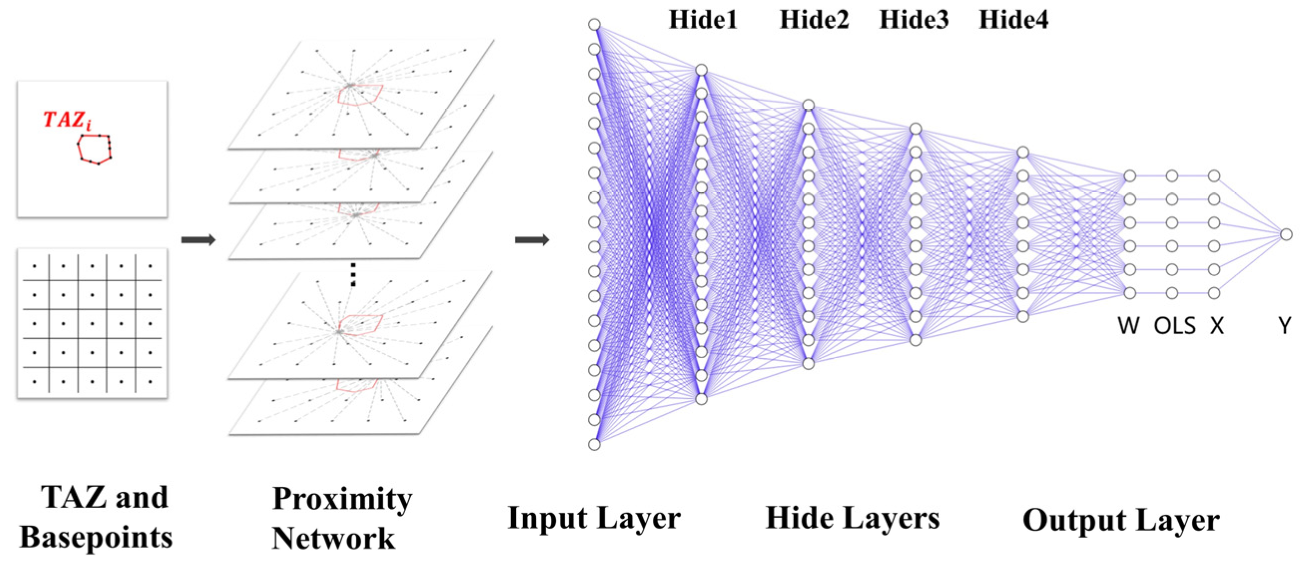
As the sample TAZs in this study range in size from 4600 to 120,000 m² and have different shapes (Figure 2), using the TAZ centroid distance alone cannot accurately express the proximity of the TAZs, leading to biased spatial weights. Therefore, the SWNN network is optimized to use the approximate shape of the TAZ as input instead of the Euclidean distance between any two sample points to construct PBNNWR. The specific construction steps are as follows:

(1)

Extract the shape features of the TAZ samples. As the TAZs in this paper were obtained from the OSM road network superimposed on impervious surfaces, most had a relatively regular shape. Therefore, taking into account the computational volume and an exhaustive description of the TAZ shape, 10 points were randomly extracted from the boundary of each TAZ, denoted as $P_i=\left[\left(u_{i1},v_{i1}\right),\left(u_{i2},v_{i2}\right),\dots ,\left(u_{i10},v_{i10}\right)\right]$. We obtained the final sample point pool $P={\left[P_1,P_2,\dots ,P_m\right]}^T$, where $m$ is the number of TAZ samples; there were 5513 TAZ samples in this study.

(2)

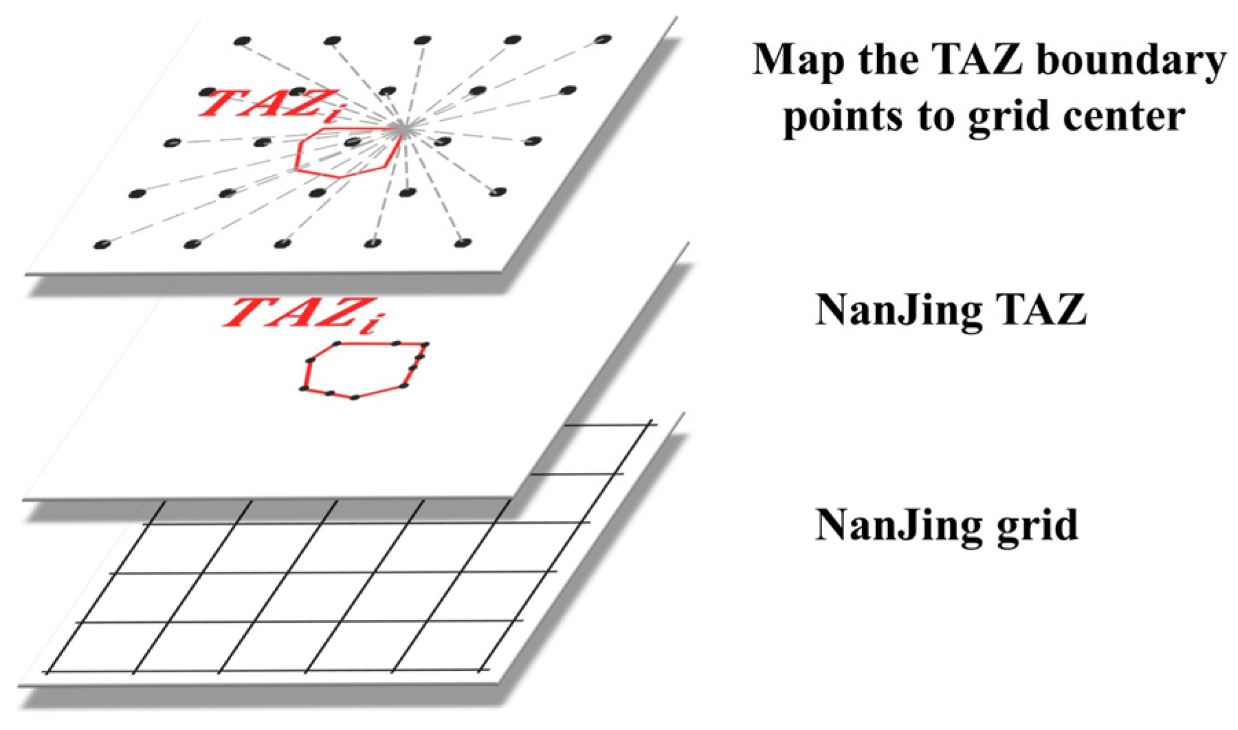
Selection of reference points. By dividing the study area into a regular grid of 3 × 3 km and using the center of the grid as the datum, 548 datum points covering the whole study area could be obtained. By calculating the distance from the ten sampling points at the boundary of each plot to all the datum points, a plot proximity relationship network was constructed (Figure 5), which represented the TAZ shape characteristics and proximity relationships between parcels. Taking $TA{Z}_i$ as an example, it could be represented in the proximity relationship network as:

$$D_i=f\left(P_i,Base\right)$$

(11)

(3)

Spatial weight calculation. Referring to the method of GWR and GNNWR to solve the weight matrix $W\left(u_i,v_i\right)$ based on the distance between sample points, $W\left(u_i,v_i\right)$ was regarded as a function of the proximity matrix $D_i$ of $TA{Z}_i$ and the spatial weights were solved using PBNNWR as follows:

$$W\left(u_i,v_i\right)=g\left(f\left(P_i,Base\right)\right)=PBNNWR\left(P_i,Base\right)=\mathrm{PBNNWR}\left(\left[\begin{array}{ccc}{d}_{1,1}^i& \cdots & d_{1,10}^i\\ ⋮& \ddots & ⋮\\ d_{k,1}^i& \cdots & d_{k,10}^i\end{array}\right]\right)$$

(12)

where $d_{k,t}^i$ denotes the Euclidean distance of the boundary sampling point $t$ of plot $i$ from the datum point $k$.

(4)

Network design. The OLS regression coefficients were calculated to represent the average relationship between each geographical element, i.e.$, \widehat{\beta }={\left(X^{T}X\right)}^{-1}{X}^{T}Y$. The spatial weights $W\left(u_i,v_i\right)$ were regarded as fluctuations of this mean relationship at different geographical locations [44], and the regression relationship was finally established. Taking TAZ $i$ as an example, the relationship can be expressed as follows:

$${\widehat{y}}_i={{\displaystyle \sum }}_{t=0}^n{\beta }_t*x_{it}={{\displaystyle \sum }}_{t=0}^n{w}_t\left(u_i,v_i\right)\ast {\beta }_{t,OLS}\ast x_{it}$$

(13)

The matrix form is ${\widehat{y}}_i=X_i^{T}W\left(u_i,v_i\right){\left(X^{T}X\right)}^{-1}{X}_i^{T}Y$, where the fitted values can be calculated from the weights, OLS regression coefficients, and independent variables. For the full TAZs in the study area, the matrix expression of PBNNWR can be obtained as follows:

$$\widehat{Y}=\left[\begin{array}{c}{\widehat{y}}_1\\ {\widehat{y}}_2\\ ⋮\\ {\widehat{y}}_m\end{array}\right]=\left[\begin{array}{c}{X}_1^T{\beta }_1\\ X_2^T{\beta }_2\\ ⋮\\ X_m^T{\beta }_m\end{array}\right]=\left[\begin{array}{c}{X}_1^{T}W\left(u_1,v_1\right){\left(X^{T}X\right)}^{-1}{X}^T\\ X_2^{T}W\left(u_2,v_2\right){\left(X^{T}X\right)}^{-1}{X}^T\\ ⋮\\ X_m^{T}W\left(u_m,v_m\right){\left(X^{T}X\right)}^{-1}{X}^T\end{array}\right]Y$$

(14)

Considering the complexity and computational cost of the network model, a six-layer PBNNWR network structure model was constructed in this paper, including one input layer, four hidden layers, and one output layer (Figure 6).

3.4.2. Model Optimization

In order to improve the goodness of fit of the influencing factors on urban vitality and ensure model complexity, LReLU [59] and Tanh [60] functions were selected as activation functions. In addition, this paper adopted the He initialization method [61] and Dropout technique [62] in each hidden layer to reduce training difficulty and improve generalization ability.

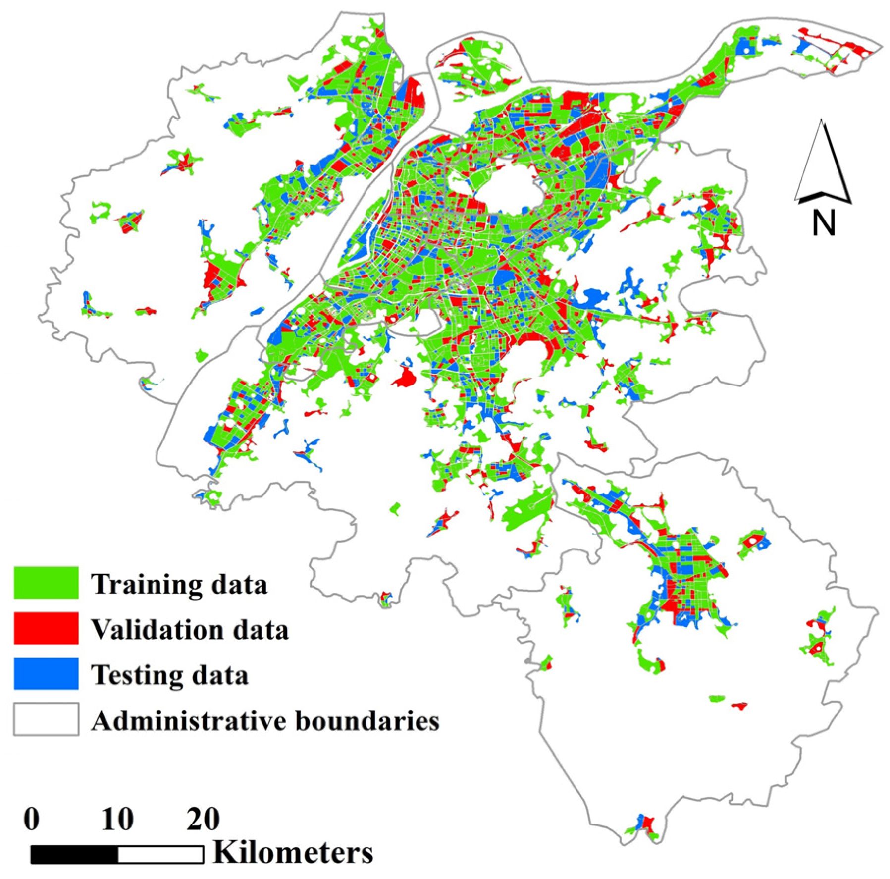
In this paper, the 5513 TAZs (Figure 2) were divided into the training set, validation set, and testing set according to a ratio of 60, 20, and 20% to ensure that the distribution of the three datasets was relatively uniform and could cover the whole study area (Figure 7). The root mean square error (RMSE) metric was selected as the loss function of the model, and the mean absolute error (MAE), Akaike information criterion (AICc), and goodness of fit (R²) were selected to evaluate model performance. During the training process, if the number of iterations in which the loss function value or R² value in the validation keeps steady exceeds a threshold (set at 200 in this paper), the model is considered over-fitted. The parameters are returned at that epoch.

4. Results

4.1. Spatial Distribution of Urban Vtality

4.1.1. Social, Economic, and Cultural Vitality

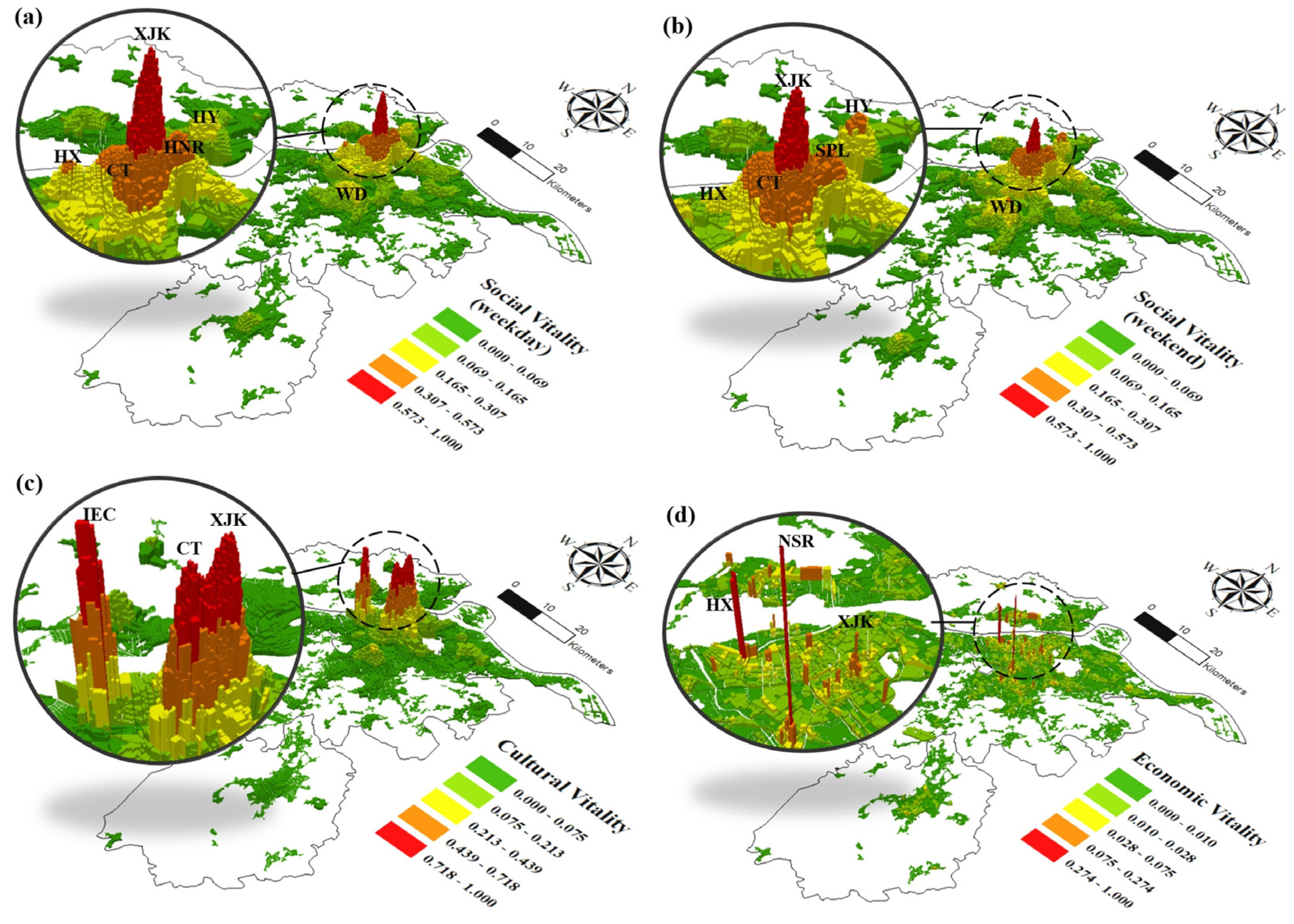
The social, economic, and cultural vitality values were calculated using mobile phone signaling data, night-time lighting data, and POI data, respectively. From the results of the natural interruption method for the hierarchical presentation of the three types of vitality, we found that social vitality on working days and rest days had a similar spatial distribution (Figure 8a,b), with the largest vitality pole located in the area of Xinjiekou (XJK), followed by Hunan Road (HNR), Sanpailou Street (SPL), and Confucius Temple (CT) around XJK. In addition, the social vitality of certain regions varied considerably over time. For example, Hexi CBD (HX) presented as a small vitality pole on weekdays and dropped significantly on weekends, whereas the social vitality around Hongyang Plaza (HY) and Wanda Plaza (WD) rose on rest days, forming two new small vitality poles, respectively. Compared with weekdays, although the peak of social vitality on rest days was smaller, there were 16.6 and 15.9% greater numbers and areas of vibrant zones (red and brown in Figure 8a,b) on weekends than on weekdays, respectively, with a total of 74 parcels and an area of 4.9 km².

The distribution of cultural vitality formed two centers, with XJK and CT districts together forming a larger area and the Nanjing International Expo Centre (IEC) district constituting a smaller area with a relatively higher vitality value (Figure 8c). The economic vitality centers are discrete, covering relatively smaller areas and forming several high and sharp columns (Figure 8d). Regarding economic vitality values, the top three places were Nanjing South Railway Station (NSR), HX, and XJK, in that order.

4.1.2. Comprehensive Urban Vitality

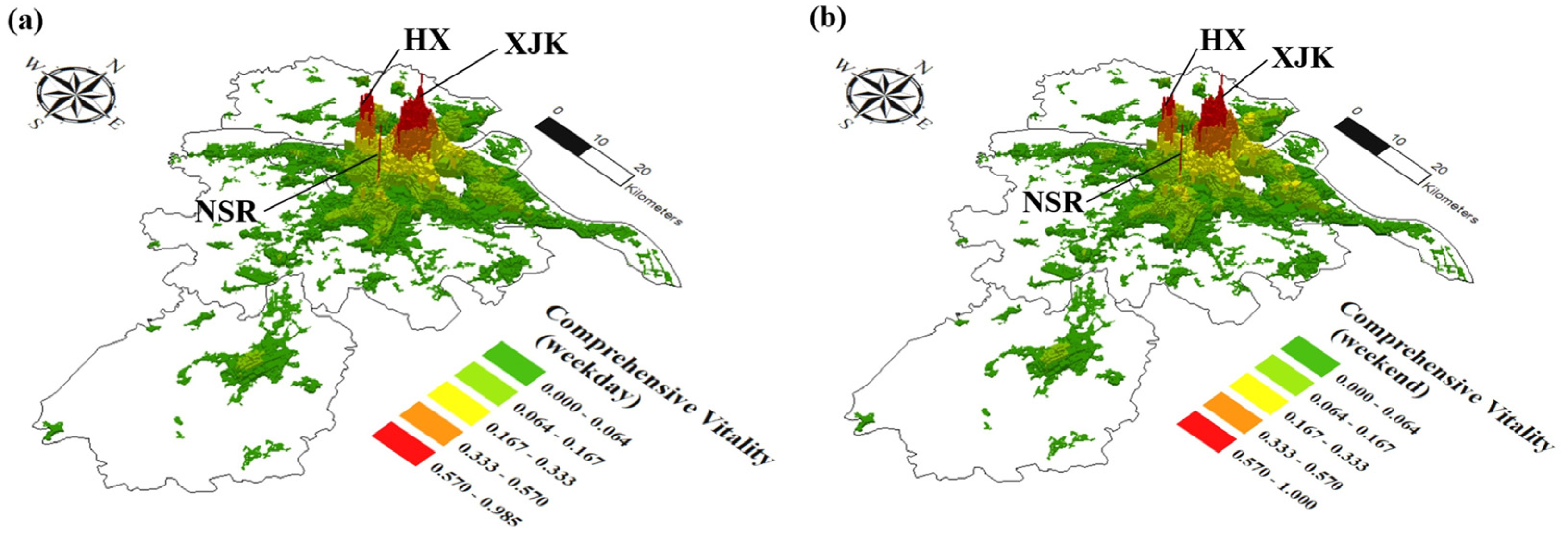
There are three high comprehensive vitality zones, XJK, HX, and NSR, covering 8.20, 1.74, and 0.03 km², respectively, on weekdays (Figure 9). The median integrated vitality zones are mainly clustered around the high vitality zones and are distributed in clusters. The difference in the distribution of vitality values between weekdays and weekends cannot be seen visually in the figure. However, statistical analyses showed that the average vitality on weekends was 6.4% higher than on weekdays, and areas with higher vitality values (red and orange color in Figure 9) on rest days (37.3 km²) were 4.5% higher than on weekdays (35.7 km²).

4.2. Statistical Characteristics of the Influencing Factors

The average VIF values of the nine indicators is 1.408, which is much less than 7.5 (

Table 3. Statistical characteristics of the impact indicators.

Variable	Max	Min	Mean	VIF	Correlation Coefficient (Weekday/Weekend)	p-Value
Net	59.80	0.00	12.70	1.141	0.229/0.238	0.005
Res	376.90	0.00	62.83	1.958	0.774/0.800	0.005
BD	11.56	0.00	0.63	1.596	0.532/0.543	0.005
Green	1.02 × 10−3	0.00	3.38 × 10−4	1.601	–0.484/–0.501	0.005
Water	500.00	0.00	312.39	1.083	0.058/0.062	0.005
Shan	2.37	0.00	1.71	1.189	0.335/0.334	0.005
HP	1.24 × 105	4437.44	2.80 × 104	1.497	0.522/0.519	0.005
Sub	1988.64	0.00	569.82	1.558	0.549/0.555	0.005
Rail	500.00	0.00	105.21	1.052	–0.154/–0.152	0.005

), indicating no co-linearity among the above indicators. Therefore, all indicators can be used to analyze the spatial heterogeneity relationship with urban vitality. Table 3 also demonstrates that the nine indicators has significant (p < 0.005) correlations with comprehensive urban vitality, with Res, BD, HP, and Sub having strong positive correlations and Green showing a strong negative correlation.

4.3. Simulation Results and Comparisons

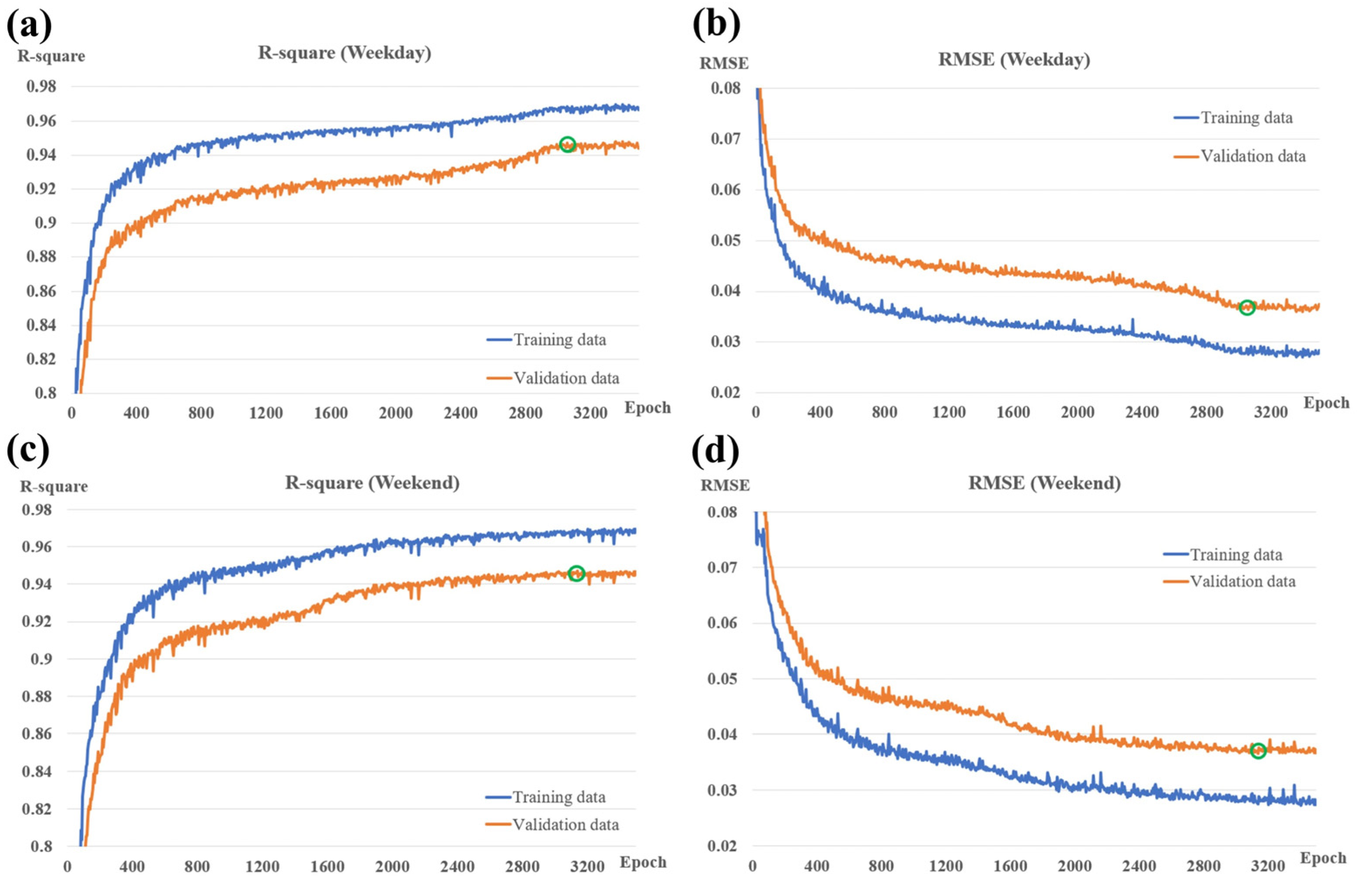
After the parameter adjustment of the PBNNWR model, the learning rate was chosen to be 0.21 and 0.25 for weekdays and weekends, respectively. The dropout ratio and batch-size were 0.3 and 64 for both weekdays and weekends. When the epoch is 3056 (green circle in Figure 10a,b), the R² and RMSEs of the validation sets reach a local optimum and remain stable while the training sets continue to be optimized; R² of the training sets and validation set are 0.968 and 0.947 and the RMSEs are 0.028 and 0.036, respectively. On rest days, the optimum is reached when the epoch is 3136, at which R² of the training and validation sets are 0.969 and 0.947 and the RMSEs are 0.028 and 0.036, respectively.

Applying the optimal model to the complete samples, the distribution of regression coefficients for the associated factors of vitality was obtained. We constructed a statistic to test the spatial non-stationarity of the regression coefficients [63], and the statistical results show that the nine associated factors significantly influenced urban vitality (

Table 4. Regression coefficients between influence indicators and urban vitality.

Variable	PBNNWR
	Min	Max	Mean	p-Value
Intercept	6.638(7.030)	15.832 (16.924)	8.039 (8.794)	0.005 ***
HP	–0.137 (–0.189)	4.226 (4.547)	0.451 (0.520)	0.005 ***
Shan	0.376 (–0.088)	8.702 (8.086)	1.773 (1.468)	0.005 ***
Net	0.063 (–0.018)	0.248 (0.027)	0.161 (0.006)	0.005 ***
BD	–0.310 (–0.191)	2.237 (2.225)	0.236 (0.444)	0.005 ***
Sub	–0.150 (–0.029)	8.379 (7.606)	1.064 (1.163)	0.005 ***
Rail	–1.076 (–1.402)	0.601 (0.459)	–0.208 (–0.247)	0.005 ***
Water	–0.194 (–0.230)	0.171 (0.317)	–0.027 (0.066)	0.005 ***
Green	–0.306 (–0.296)	–0.138 (–0.128)	–0.212 (–0.214)	0.005 ***
Res	4.579 (4.370)	13.192 (13.829)	5.989 (6.576)	0.005 ***

Note: Data in brackets represent regression coefficients on weekends; the values for all indicators are expanded by a factor of 100 due to space limitations; *** indicates a significance level of 0.005.

). Res, Sub, Shan, HP, Net, and BD all had a positive relationship with urban vitality, whereas Rail and Green had a depressing effect on urban vitality. For Water, there was an opposite effect on weekdays and weekends, with average contributions of –0.027 and 0.066%, respectively.

The OLS, GWR, and GNNWR models were selected for comparison, where two common kernel function types [43], GWR-FG (the fixed Gaussian kernel) and GWR-AB (the adaptive bivariate kernel), were chosen for the GWR model. The different modeling results had the same trends on weekdays and weekends. Therefore, only weekday results were selected for later analysis (

Table 5. Statistics of the different modeling results on weekdays.

Model	Training Result				Validation Result			Testing Result
	R2	RMSE	MAE	AICc	R2	RMSE	MAE	R2	RMSE	MAE
OLS	0.687	0.087	0.054	−16,153.7	0.652	0.093	0.056	0.662	0.083	0.052
GWR-FG	0.891	0.051	0.027	−19,631.4	0.878	0.055	0.028	0.893	0.047	0.023
GWR-AB	0.946	0.036	0.020	−21,941.9	0.838	0.063	0.036	0.851	0.055	0.031
GNNWR	0.931	0.040	0.024	−21,271.6	0.893	0.052	0.026	0.896	0.047	0.025
PBNNWR	0.968	0.028	0.018	−23,741.1	0.947	0.036	0.020	0.956	0.030	0.018

). For the training dataset, the OLS model performed the worst, and the PBNNWR model gave the best results, based on the four metrics of R², RMSE, MAE, and AICc. GNNWR outperformed GWR-FG, but did not perform as well as GWR-AB. Compared with OLS, GWR-FG, GWR-AB, and GNNWR, PBNNWR improved its R² by approximately 28, 8, 2, and 4%, respectively.

For the testing dataset, the OLS model also performed the worst. In contrast to the training dataset, GWR-FG and GNNWR significantly outperform GWR-AB. The PBNNWR model is greatly superior to other models with an R² of 0.956 (Table 5).

5. Discussion

5.1. Analysis of Simulation Results of the PBNNWR Model

The OLS model performed the worst compared with other models (Table 5). This is because OLS only constructed an average relationship between urban vitality and its influencing factors. The Moran’s I values for driving factors (from 0.2 to 0.8) and comprehensive vitality (0.82) reveal that the spatial distribution of both independent and dependent variables had highly significant (p < 0.001) autocorrelations. Thus, a local regression model, such as GWR, that considers spatial autocorrelation has efficient explanatory power of local variations in urban dynamics. This discovery is similar to what Li and Wu et al. [64] have found.

Comparing the GWR-AB and GWR-FG models, the former’s simulation results were significantly better than that of the latter, as GWR-FG chooses a fixed bandwidth in the kernel function, which is insufficient to reflect the complex spatial variations between the independent and dependent variables in practice [65]. In contrast, the GWR-AB model is based on the density of geographical elements and sets the adaptive bandwidth by finding the optimal number of neighbors, which is more suitable for TAZs (Figure 2). Our study shows the importance of choosing the type of kernel function for GWR models, and the feasibility of using neural networks to improve kernel functions to enhance model performance, which has also been demonstrated by Wu and Wang et al. [43].

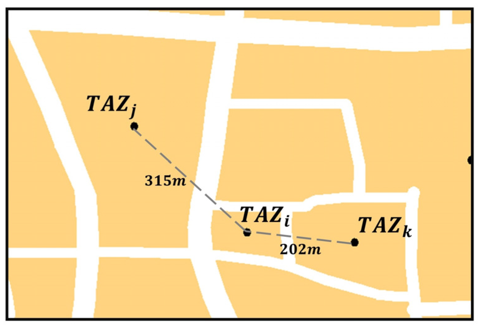
Table 5 shows that the GNNWR simulations on the training dataset outperform GWR-FG, demonstrating the improved effect of the neural network on the kernel function. However, the GNNWR results are slightly worse than GWR-AB, which may be related to the choice of TAZ proxies. The parcel samples were collected from the overlay of the OSM road buffers and impervious surfaces with irregular shapes ranging in size from 4600 to 120,000 m². However, both GWR and GNNWR selected only the centroid as the parcel proxy, so neighboring TAZs of different sizes may give rise to an overestimation of the distance between two parcels. For example, in Figure 11, $TA{Z}_i$ is adjacent to $TA{Z}_j$ and $TA{Z}_k$, and the distance between two adjacent parcels is less than 50 m if measured by the boundary distance. However, the $d_{ij}$ and $d_{ik}$ calculated based on the centroid are 315 and 202 m, respectively, which are much larger than the actual distance of the two parcels, leading to some deviation in the spatial weights $W_j\left(u_i,v_i\right)$ and $W_k\left(u_i,v_i\right)$ solved by using GWR or GNNWR.

In order to solve the above problems, several boundary points have been selected to form a regular grid. The shape and spatial relationships of TAZs were represented by the attributes of the grid points (Figure 5), and the spatial weight was calculated by the neural network. The PBNNWR model explained 96.8% of the spatial variation in vitality, which was higher than GWR-AB (94.6%) and GNNWR (93.1%). For the testing dataset, the prediction performance of PBNNWR (R² = 0.956) also far exceeded that of the other models (Table 5). The GWR-AB model, which had the second highest training accuracy, for example, had significantly lower prediction performance (R² = 0.85), indicating that GWR-AB suffered from overfitting. The above results demonstrate that the spatial centroids of irregularly sized and shaped parcels cannot be used to calculate the spatial weights in regression models. By adding TAZ boundaries, the PBNNWR model created in this study can more accurately capture the non-linear relationships between geographic elements and better solve spatial weight and fit and predict urban vibrancy.

5.2. Spatial Heterogeneity in Different Types of Urban Vitality

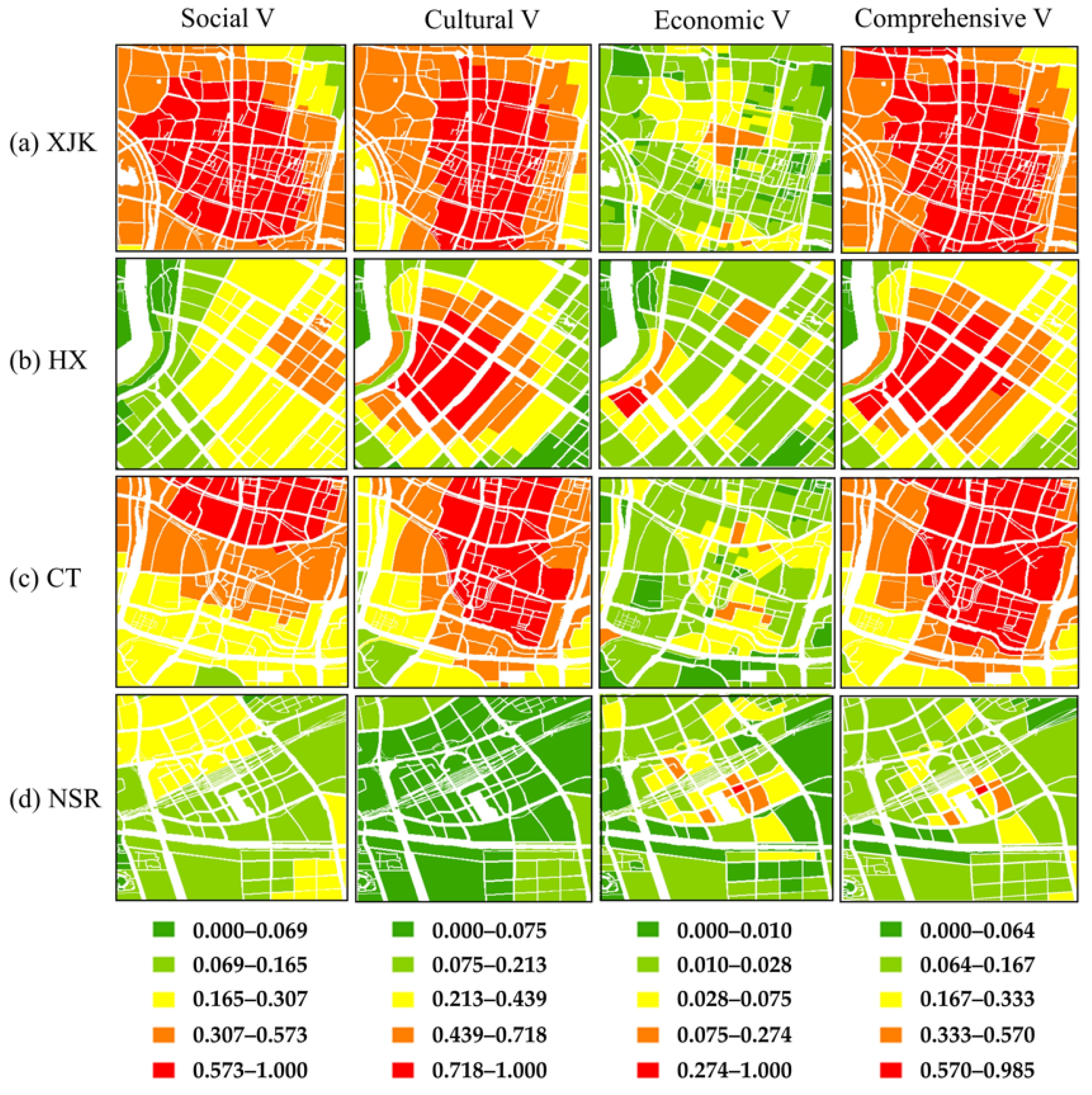
In an era of big data, data such as mobile phone user data, social media data, and POI can help us perceive urban dynamics on a large scale and explore the distribution of urban vitality by providing objective and real-time information [66]. However, inconsistencies in data sources may lead to a significant difference in the revealed urban vitality [26]. Here, four typical zones were selected to illustrate the differences in the spatial distributions of social, economic, and cultural vitality, and the combined effect of comprehensive vitality (Figure 12).

The XJK CBD, as “the first Chinese business district”, has a large number of shopping malls, retail, restaurants, and entertainment facilities, which have a strong ability to attract people. However, there is some difference in their vitality centers (Figure 12a). Both mobile phone data and night-time lighting data reveal its centroid as the location of the vitality center. At the same time, cultural POI data show that the vitality center is shifted eastward because of of the many museums, libraries, art galleries, and cultural and sports centers in this area. The distribution of comprehensive vitality also shows high social and economic vitality within the core area and high cultural vitality in the eastern part of the core area.

The Hexi CBD (HX) is a combination of financial information, software development, business offices, and cultural expo centers. Although its social vitality is low, its cultural and economic vitality are at the forefront in Nanjing (Figure 12b). Comprehensive vitality is similar to cultural vitality, but the range has expanded due to the economic vitality represented by night-light data.

The Confucius Temple (CT) was the cultural and educational center in the Ming and Qing dynasties. It has the highest cultural vitality values in Nanjing, but its social and economic vitality have no corresponding dominant positions (Figure 12c). The distribution of comprehensive vitality in CT takes into account the high value of social vitality in the eastern region and the high value of cultural vitality in the southern region. Nanjing South Railway Station (NSR) is the largest transportation hub in East China and the largest railway station in Asia, with a daily passenger volume of 400,000 in 2019 [67], which has led to economic development around this area. However, its vitality is almost zero based on cultural POIs (Figure 12d). Based on our calculations, NSR was mainly divided into low and medium value areas of comprehensive vitality.

Therefore, comprehensive vitality integrates the three parts of the vitality distribution from different data sources and can give a more exhaustive picture of the vitality distribution in Nanjing. The distribution of the comprehensive vitality classifications in this paper is similar to the results provided by Tang and Xu et al. [68] using the spatial TOPSIS method.

5.3. The Relationship between Vitality and Driving Factors

The distribution of comprehensive vitality in Nanjing shows significant spatial heterogeneity (Figure 9). The study of the influence of the natural environment and social and economic factors on vitality can provide theoretical guidance for optimizing the spatial layout and resource allocation of the city. The spatial distribution of the regression coefficients of different influencing factors and urban vitality, based on the results of the PBNNWR model, were plotted in the following figures. The coefficients were graded by the natural interruption method, with values near 0 being manually set to 0 as a threshold for distinguishing the positive or negative impacts of drivers on urban vitality [69]. This section focuses on weekdays as an example. For regression coefficients with a significant difference in distribution, both weekdays and weekends were analyzed.

For HP (Figure 13a), the areas with the highest regression coefficients are XJK and HX, which have higher housing prices and are accompanied by convenient transport, adequate commercial business, public service facilities, and other elements with vibrancy-creating functions. The above results have also been found by Wu and Ye et al. [24] and Lu et al. [33]. However, the peak area of HP does not precisely match the peak area of the regression coefficients. In Nanjing city, the highest house prices are highly related to some primary and secondary schools with high teaching quality (marked in numbers in Figure 13b), regardless of whether the environmental conditions are poor, such as in XJK and the south of XW, or good, such as in LJ and HX. The improvement of educational resources and supporting facilities has led to extremely high residential prices and strong vitality [70], and will gradually appreciate over time [71]. However, urban vitality in these education districts would not grow indefinitely with housing prices. From the HP regression coefficients, the vitality only increases by 0.015 to 0.029% for every 1% increase in housing price.

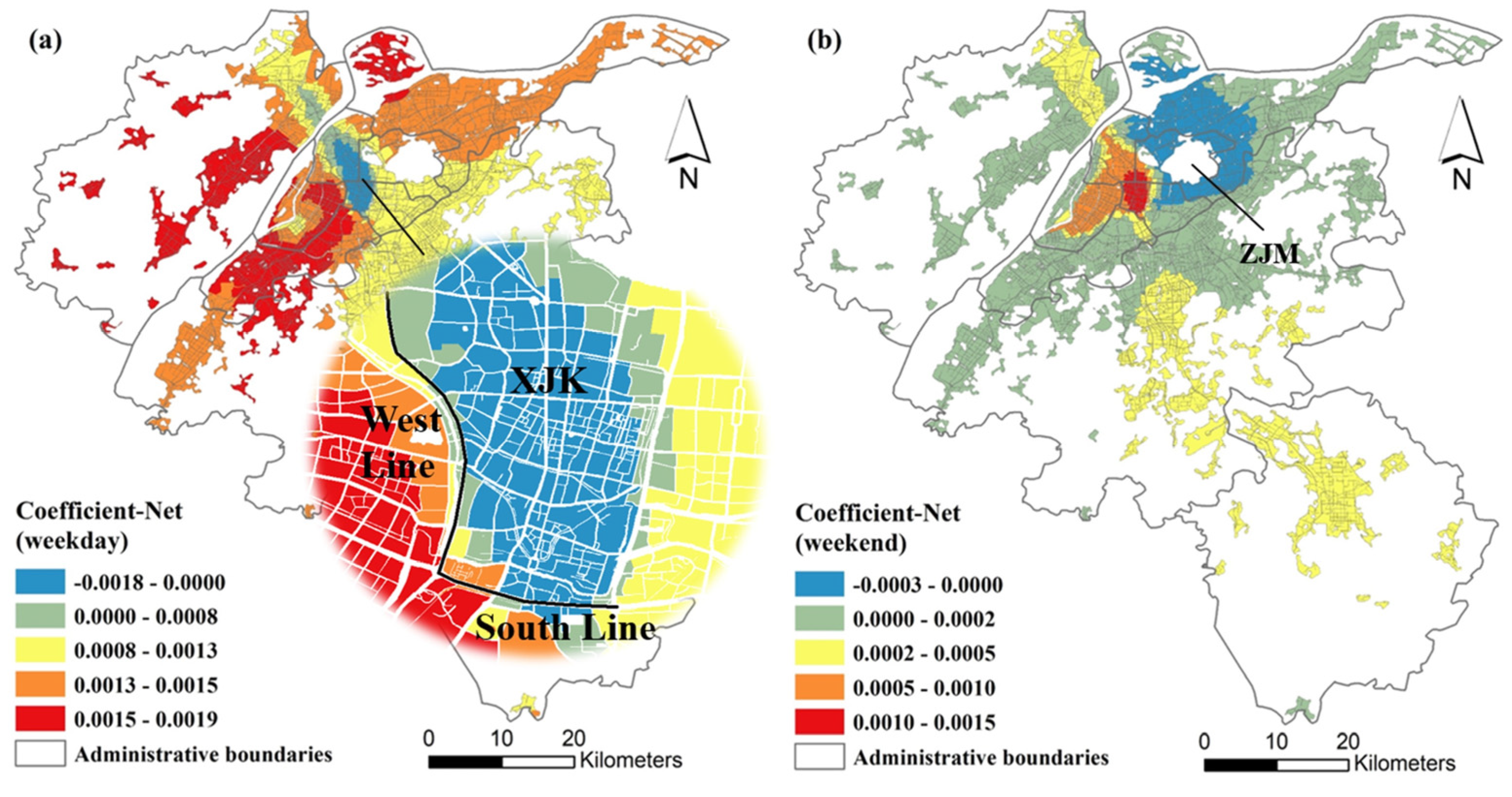
A well-developed road network provides citizens with a variety of path options and creates a wide range of social activities by increasing pedestrian exposure. Thus, the Net has a positive relationship with urban vitality [52,64]. However, in our study, Net presented a suppressing effect on urban vitality for the area around XJK on weekdays and Zijin Mountain (ZJM) on weekends (Figure 14a,b). This result may be explained in terms of data. The existence of underground expressways along the west line of the inner ring and a large number of viaducts along the south line of the inner ring makes the road network density in the areas around the centers higher than that in the core areas, resulting in a “high vitality–low Net” and “low vitality–high Net” situation in XJK. For ZJM, the vitality and Net in the surrounding parcels were counted, and the results showed that the comprehensive vitality and Net were not strictly correlated in these TAZs. The absolute value of its regression coefficient (less than 0.0003) also proves this view.

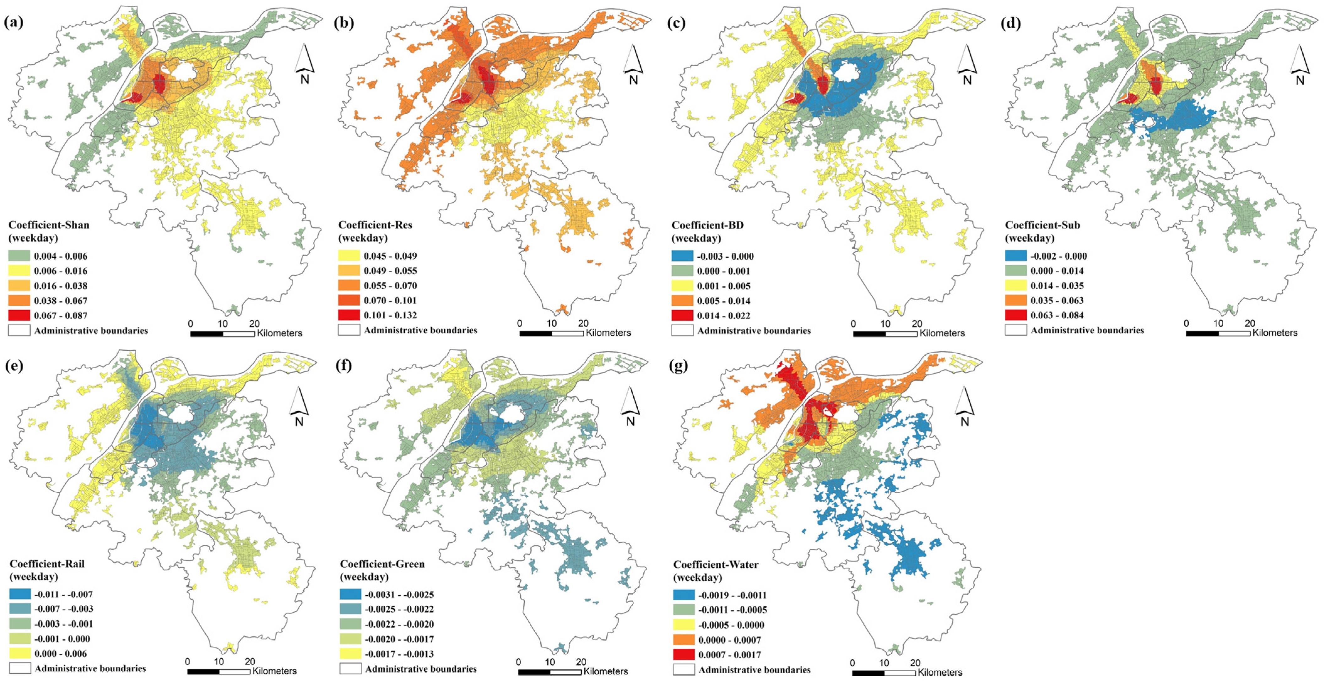
The regression coefficients for Shan and Res show positive values throughout the study area and have a similar distribution (Figure 15a,b). Obviously, people tend to live in functionally rich and well-equipped areas, and adequate services and diverse urban functions are necessary to stimulate economic and social vitality [22,51]. In the agricultural, industrial, and natural landscape cover areas in the periphery of the city, the concentration of vitality is associated with its dominant land function [72]; thus, the regression coefficients for Shan are both at low values. Both BD and Sub contribute to urban vitality, and the urban core contributes the most. The higher BD (Figure 15c) in the core area helps to improve land use efficiency and host more facilities and human activities [42,73]. However, to protect the ancient cultural capital of Nanjing, the government adopted height restrictions in 2011. Therefore, the creation of vibrancy around the core area has little to do with BD.

Rail and Green act as a disincentive to urban vitality (Figure 15e,f), due to the fact that rail segregates urban space to a certain extent and is not conducive to human activities [38,51]. Similarly, high vegetation cover areas, e.g., parks, neighborhood greenery, and mountainous areas, are large, with a relatively lower built-up density and a single function [74], leading to low vitality. Water has positive or negative influences on vitality (Figure 15g), depending on the varying areas. The positive coefficients are mainly distributed along the banks of the Yangtze River, indicating that mature waterfront areas can attract human activities to an extent [38]. In the southeast, water bodies are mostly interspersed in villages and ecological landscape areas, which are less vibrant and show a negative correlation between urban vitality and Water overall.

6. Conclusions

This paper used mobile phone data, POI data, and night-time lighting data to quantify comprehensive urban vitality and constructed an index system of vitality drivers through multiple sources of big data such as OSM and building density. We designed a plot boundary-based neural network weighted regression model to analyze the spatial heterogeneity relationship between urban vitality and its drivers. This study found that a single source of urban data (mobile phone data, POI, night light remote sensing data) only revealed a certain aspect of vitality. In contrast, the comprehensive indicator calculated using multiple sources of big data could provide a comprehensive picture of urban vitality. The PBNNWR model designed in this paper could effectively capture the relationship between urban vitality and influencing factors. Taking weekdays as an example, the fitting accuracy and prediction accuracy of PBNNWR for urban vitality reached 96.8 and 95.6%, respectively, with prediction accuracy improved by 29.4, 6.3, and 6.1%, and RMSE reduced by 63.8, 36.2, and 36.2% when compared with the OLS, GWR and GNNWR models, respectively. According to the regression results of the model, the positive or negative influences of the associated indicators on vitality depended on the location. In most areas, house prices, functional diversity, road network density, building density, metro station accessibility, and residential facility density showed a positive correlation with urban vitality. Railway accessibility, hydrophilicity, and green space coverage could weaken urban vitality. Designers could refer to these results to build up local vitality using aspects of the physical environment, social economy, and so on.

In this paper, we used a neural network to solve the spatial weight, which overcame the problem that traditional regression models have when simple kernel functions cannot adequately fit the complex non-linear relationships among geographic elements. In addition, the GWR and GNNWR models used in previous studies calculate spatial weights through the centroid of geographic elements, which is inadequate when dealing with parcels with different shapes and sizes. The PBNNWR model more adequately fit the spatially non-stationarity relationships between urban vitality and influencing factors by considering parcel size and shape when measuring parcel proximity. Of course, although PBNNWR performs well in modeling, it is much less computationally efficient than the GWR model. Therefore, PBNNWR is suitable for complex geographic relationships, whereas GWR is a better choice for simple spatial relationship studies.

This study still leaves room for future explorations. First, due to the limitations of the data source, only one scene of night light remote sensing image with high quality was selected to calculate economic vitality, and the temporal resolution was low compared with mobile phone data. The difference in comprehensive vitality between weekdays and weekends in this paper was mostly related to the social vitality characterized by mobile phone user data. Weibo is the largest social media platform in China and, similar to Twitter, supports users to post reviews, daily tasks, etc., with location. Dianping supports users to rate and recommend consumption places in China. These data had high temporal resolution and should be considered in the future to represent economic vitality [25,51]. Then, the spatial heterogeneity of the influencing factors on urban vitality has only been studied for weekdays and weekends. Researchers have explored the spatiotemporal non-stationarity relationship using the geographically and temporally weighted regression (GTWR) model using mobile phone data or Weibo check-in data [24,75]. In the future, the design of a spatiotemporal weighted regression neural network model should be considered. This could be used to assess the temporal properties of mobile user data to explore the distribution of vitality and changes in the influence mechanism at an hourly level.

References

1. UN. World Urbanization Prospects Report. Available online: https://www.un.org/development/desa/zh/news/population/2018-world-urbanization-prospects.html (accessed on 14 October 2022).
2. Xu, L.; Ge, J.; Hua, Y. Analysis on the environmental problems accompanying the high-speed urbanization of small towns in China. J. Environ. Sci. 2002, 14, 120–126. [Google Scholar]
3. Jin, X.; Long, Y.; Sun, W.; Lu, Y.; Yang, X.; Tang, J. Evaluating cities’ vitality and identifying ghost cities in China with emerging geographical data. Cities 2017, 63, 98–109. [Google Scholar] [CrossRef]
4. Liu, X.; Cao, G.; Liu, T.; Liu, H. Semi-urbanization and evolving patterns of urbanization in China: Insights from the 2000 to 2010 national censuses. J. Geogr. Sci. 2016, 26, 1626–1642. [Google Scholar] [CrossRef]
5. Li, Y.; Jia, L.; Wu, W.; Yan, J.; Liu, Y. Urbanization for rural sustainability–rethinking China’s urbanization strategy. J. Clean. Prod. 2018, 178, 580–586. [Google Scholar] [CrossRef]
6. Lynch, K. A Theory of Good City Form; MIT Press: Boston, MA, USA, 1981. [Google Scholar]
7. Fang, C.; He, S.; Wang, L. Spatial Characterization of Urban Vitality and the Association With Various Street Network Metrics From the Multi-Scalar Perspective. Front. Public Health 2021, 9, 677910. [Google Scholar] [CrossRef] [PubMed]
8. Ye, Y.; Zhuang, Y.; Zhang, L.; Van Nes, A. Designing Urban Spatial Vitality from Morphological Perspective—A Study Based on Quantified Urban Morphology and Activities’ Testing. Int. Urban Plan. 2016, 31, 26–33. [Google Scholar]
9. Jacobs, J. The Death and Life of Great American Cities; Random House: New York, NY, USA, 1961. [Google Scholar]
10. Montgomery, J. Making a city: Urbanity, vitality and urban design. J. Urban Des. 1998, 3, 93–116. [Google Scholar] [CrossRef]
11. Gehl, J. New City Spaces; Danish Architectural Press: Copenhagen, Denmark, 2000. [Google Scholar]
12. Jin, Y. Study on Urban Economic Vitality Index in China. Sci. Geogr. Sin. 2007, 27, 9–16. [Google Scholar]
13. Turok, I.; Mykhnenko, V. The trajectories of European cities 1960–2005. Cities 2007, 24, 165–182. [Google Scholar] [CrossRef]
14. Zhou, W.; Yan, J. Urban Economics; Fudan University Press: Shanghai, China, 2004. (In Chinese) [Google Scholar]
15. Jiang, D. The Theory of City Form Vitality; Southeast University Press: Nanjing, China, 2007. (In Chinese) [Google Scholar]
16. Ta, N.; Zeng, Y.; Zhu, Q.; Wu, J. Relationship between Built Environment and Urban Vitality in Shanghai Downtown Area based on Big Data. Sci. Geogr. Sin. 2020, 40, 60–68. [Google Scholar]
17. Zarin, S.; Niroomand, M.; Heidari, A. Physical and social aspects of vitality case study: Traditional street and modern street in Tehran. Procedia-Soc. Behav. Sci. 2015, 170, 659–668. [Google Scholar] [CrossRef] [Green Version]
18. Yue, W.; Chen, Y.; Thy, P.T.M.; Fan, P.; Liu, Y.; Zhang, W. Identifying urban vitality in metropolitan areas of developing countries from a comparative perspective: Ho Chi Minh City versus Shanghai. Sustain. Cities Soc. 2021, 65, 102609. [Google Scholar] [CrossRef]
19. Montalto, V.; Moura, C.J.T.; Langedijk, S.; Saisana, M. Culture counts: An empirical approach to measure the cultural and creative vitality of European cities. Cities 2019, 89, 167–185. [Google Scholar] [CrossRef]
20. Yang, J.; Cao, J.; Zhou, Y. Elaborating non-linear associations and synergies of subway access and land uses with urban vitality in Shenzhen. Transp. Res. Part A Policy Pract. 2021, 144, 74–88. [Google Scholar] [CrossRef]
21. Huang, B.; Wang, J. Big Spatial Data for Urban and Environmental Sustainability. Geo-Spat. Inf. Sci. 2020, 23, 125–140. [Google Scholar] [CrossRef]
22. Liu, S.; Zhang, L.; Long, Y.; Long, Y.; Xu, M. A new urban vitality analysis and evaluation framework based on human activity modeling using multisource big data. ISPRS Int. J. Geo-Inf. 2020, 9, 617. [Google Scholar] [CrossRef]
23. Kim, S. Urban Vitality, Urban Form, and Land Use: Their Relations within a Geographical Boundary for Walkers. Sustainability 2020, 12, 10633. [Google Scholar] [CrossRef]
24. Wu, C.; Ye, X.; Ren, F.; Du, Q. Check-in behaviour and spatio-temporal vibrancy: An exploratory analysis in Shenzhen, China. Cities 2018, 77, 104–116. [Google Scholar] [CrossRef]
25. Long, Y.; Huang, C. Does block size matter? The impact of urban design on economic vitality for Chinese cities. Environ. Plan. B Urban Anal. City Sci. 2019, 46, 406–422. [Google Scholar] [CrossRef] [Green Version]
26. Tu, W.; Zhu, T.; Xia, J.; Zhou, Y.; Lai, Y.; Jiang, J.; Li, Q. Portraying the spatial dynamics of urban vibrancy using multisource urban big data. Comput. Environ. Urban Syst. 2020, 80, 101428. [Google Scholar] [CrossRef]
27. Zhang, A.; Li, W.; Wu, J.; Lin, J.; Chu, J.; Xia, C. How can the urban landscape affect urban vitality at the street block level? A case study of 15 metropolises in China. Environ. Plan. B Urban Anal. City Sci. 2021, 48, 1245–1262. [Google Scholar] [CrossRef]
28. Wang, P.; Liu, K.; Wang, D.; Fu, Y. Measuring urban vibrancy of residential communities using big crowdsourced geotagged data. Front. Big Data 2021, 4, 690970. [Google Scholar] [CrossRef]
29. Yue, Y.; Zhuang, Y.; Yeh, A.G.O.; Xie, J.Y.; Ma, C.L.; Li, Q.Q. Measurements of POI-based mixed use and their relationships with neighbourhood vibrancy. Int. J. Geogr. Inf. Sci. 2017, 31, 658–675. [Google Scholar] [CrossRef] [Green Version]
30. Chen, S.L.; Chen, H.H.; Li, X. The ability of nighttime imagery in monitoring economic activity in different scales. Sci. Geogr. Sin. 2020, 40, 1476–1483. [Google Scholar]
31. Doll, C.; Muller, J.P.; Morley, J. Mapping regional economic activity from nighttime light satellite imagery. Ecol. Econ. 2006, 57, 75–92. [Google Scholar] [CrossRef]
32. Lan, F.; Gong, X.; Da, H.; Wen, H. How do population inflow and social infrastructure affect urban vitality? Evidence from 35 large- and medium-sized cities in China. Cities 2020, 100, 102454. [Google Scholar] [CrossRef]
33. Lu, S.; Shi, C.; Yang, X. Impacts of Built Environment on Urban Vitality: Regression Analyses of Beijing and Chengdu, China. Int. J. Environ. Res. Public Health 2019, 16, 4592. [Google Scholar] [CrossRef] [Green Version]
34. Wayne, A.; Logan, D. American Urban Architecture: Catalysts in the Design of Cities; University of California Press: Berkeley, CA, USA, 1989. [Google Scholar]
35. Lu, S.; Huang, Y.; Shi, C.; Yang, X. Exploring the Associations Between Urban Form and Neighborhood Vibrancy: A Case Study of Chengdu, China. ISPRS Int. J. Geo-Inf. 2019, 8, 165. [Google Scholar] [CrossRef] [Green Version]
36. Sung, H.; Lee, S. Residential built environment and walking activity: Empirical evidence of Jane Jacobs’ urban vitality. Transp. Res. Part D Transp. Environ. 2015, 41, 318–329. [Google Scholar] [CrossRef]
37. Zeng, C.; Song, Y.; He, Q.; Shen, F. Spatially explicit assessment on urban vitality: Case studies in Chicago and Wuhan. Sustain. Cities Soc. 2018, 40, 296–306. [Google Scholar] [CrossRef]
38. Wu, W.; Niu, X. Influence of built environment on urban vitality: Case study of Shanghai using Mobile phone location data. J. Urban Plan. Dev. 2019, 145, 04019007. [Google Scholar] [CrossRef]
39. Dong, Y.H.; Peng, F.L.; Guo, T.-F. Quantitative assessment method on urban vitality of metro-led underground space based on multisource data: A case study of Shanghai Inner Ring area. Tunn. Undergr. Space Technol. 2021, 116, 104108. [Google Scholar] [CrossRef]
40. Yue, W.; Chen, Y.; Zhang, Q.; Liu, Y. Spatial Explicit Assessment of Urban Vitality Using Multi-Source Data: A Case of Shanghai, China. Sustainability 2019, 11, 638. [Google Scholar] [CrossRef] [Green Version]
41. Gan, X.; Huang, L.; Wang, H.; Mou, Y.; Wang, D.; Hu, A. Optimal block size for improving urban vitality: An exploratory analysis with multiple vitality indicators. J. Urban Plan. Dev. 2021, 147, 1–12. [Google Scholar] [CrossRef]
42. Wang, N.; Wu, J.; Li, S.; Wang, H.; Peng, Z. Spatial Features of Urban Vitality and the Impact of Built Environment on Them Based on Multi-Source Data: A Case Study of Shenzhen. Trop. Geogr. 2021, 41, 1280–1291. [Google Scholar]
43. Wu, S.; Wang, Z.; Du, Z.; Huang, B.; Zhang, F.; Liu, R. Geographically and temporally neural network weighted regression for modeling spatiotemporal non-stationary relationships. Int. J. Geogr. Inf. Sci. 2020, 35, 582–608. [Google Scholar] [CrossRef]
44. Du, Z.; Wang, Z.; Wu, S.; Zhang, F.; Liu, R. Geographically neural network weighted regression for the accurate estimation of spatial non-stationarity. Int. J. Geogr. Inf. Sci. 2020, 34, 1353–1377. [Google Scholar] [CrossRef]
45. Globalization and World Cities Research Network. Available online: https://detailedpedia.com/wiki-Globalization_and_World_Cities_Research_Network (accessed on 30 November 2022).
46. Gong, P.; Chen, B.; Li, X.; Liu, H.; Wang, J.; Bai, Y.; Chen, J.; Chen, X.; Fang, L.; Feng, S.; et al. Mapping essential urban land use categories in China (EULUC-China): Preliminary results for 2018. Sci. Bull. 2020, 65, 182–187. [Google Scholar] [CrossRef] [Green Version]
47. Zhang, X.; Du, S.; Wang, Q. Hierarchical semantic cognition for urban functional zones with VHR satellite images and POI data. ISPRS J. Photogramm. Remote Sens. 2017, 132, 170–184. [Google Scholar] [CrossRef]
48. Sun, J.; Wang, H.; Song, Z.; Lu, J.; Meng, P.; Qin, S. Mapping Essential Urban Land Use Categories in Nanjing by Integrating Multisource Big Data. Remote Sens. 2020, 12, 2386. [Google Scholar] [CrossRef]
49. Li, X.; Gong, P.; Zhou, Y.; Wang, J.; Bai, Y.; Chen, B.; Hu, T. Mapping Global Urban Boundaries from the Global Artificial Impervious Area (GAIA) Data. Environ. Res. Lett. 2020, 15, 094044. [Google Scholar] [CrossRef]
50. Zhao, H.; Yu, D.; Miao, C.; Li, G.; Feng, Y.; Bie, Q. The Location Distribution Characteristics and Influencing Factors of Cultural Facilities in Zhengzhou Based on POI Data. Sci. Geogr. Sin. 2018, 38, 1525–1534. [Google Scholar]
51. Huang, B.; Zhou, Y.; Li, Z.; Song, Y.; Cai, J.; Tu, W. Evaluating and characterizing urban vibrancy using spatial big data: Shanghai as a case study. Environment and Planning B. Urban Anal. City Sci. 2020, 47, 1543–1559. [Google Scholar]
52. Zhu, T.; Tu, W.; Le, Y.; Zhong, C.; Zhao, T.; Li, Q.; Li, Q. Sensing urban vibrancy using geo-tagged data. Acta Geod. Cartogr. Sin. 2020, 49, 365–374. [Google Scholar]
53. Li, X.; Shao, X.; Li, R. Optimization of tobacco water-fertilizer coupling scheme under effective microorganisms biochar-based fertilizer application condition. Agron. J. 2021, 113, 1–11. [Google Scholar] [CrossRef]
54. Li, C.X.; Ma, Y.F.; Zhang, Y.; Wei, Y. Dynamic evolution mode of regional dominance indexes of Chinese inbound tourism flows during 1993 to 2008: An empirical research based on modified entropy technology. Geogr. Res. 2012, 31, 257–268. [Google Scholar]
55. Zou, Z.; Sun, J.; Ren, G. Study and Application on the Entropy method for Determination of Weight of evaluating indicators in Fuzzy Synthetic Evaluation for Water Quality Assessment. Acta Sci. Circumst. 2005, 4, 552–556. [Google Scholar]
56. Ye, Y.; Li, D.; Liu, X. How block density and typology affect urban vitality: An exploratory analysis in Shenzhen, China. Urban Geogr. 2018, 39, 631–652. [Google Scholar] [CrossRef]
57. Zhang, X.; Wu, S.; Zhao, Z. Spatial distribution characteristics of people with small activity space in urban based on mobile phone signaling data. J. Geo-Inf. Sci. 2021, 23, 1433–1445. [Google Scholar]
58. Fu, R.; Zhang, X.; Yang, D.; Cai, T.; Zhang, Y. The Relationship between Urban Vibrancy and Built Environment: An Empirical Study from an Emerging City in an Arid Region. Int. J. Environ. Res. Public Health 2021, 18, 525. [Google Scholar] [CrossRef]
59. Andrew, M.; Awni, H.; Andrew, N. Rectifier Nonlinearities Improve Neural Network Acoustic Models. In Proceedings of the International Conference on Machine Learning: Workshop on Deep Learning for Audio Speech and Language Processing, Atlanta, GA, USA, 16 June 2013. [Google Scholar]
60. Glorot, X.; Bordes, A.; Bengio, Y. Deep sparse rectifier neural networks. In Proceedings of the Fourteenth International Conference on Artificial Intelligence and Statistics, Ft. Lauderdale FL, USA, 11–13 April 2011; JMLR Workshop and Conference Proceedings. pp. 315–323. [Google Scholar]
61. He, K.; Zhang, X.; Ren, S.; Sun, J. Delving deep into rectifiers: Surpassing human-level performance on ImageNet classification. In Proceedings of the 2015 IEEE International Conference on Computer Vision (ICCV), Santiago, Chile, 7–13 December 2015; IEEE: Piscataway, NJ, USA, 2015; pp. 1026–1034. [Google Scholar] [CrossRef] [Green Version]
62. Srivastava, N.; Hinton, G.; Krizhevsky, A.; Sutskever, I.; Salakhutdinov, R. Dropout: A Simple Way to Prevent Neural Networks from Overfitting. J. Mach. Learn. Res. 2014, 15, 1929–1958. [Google Scholar]
63. Leung, Y.; Mei, C.; Zhang, W. Statistical Tests for Spatial Nonstationarity Based on the Geographically Weighted Regression Model. Environ. Plan. A Econ. Space 2000, 32, 9–32. [Google Scholar] [CrossRef] [Green Version]
64. Li, S.; Wu, C.; Lin, Y.; Li, Z.; Du, Q. Urban Morphology Promotes Urban Vibrancy from the Spatiotemporal and Synergetic Perspectives: A Case Study Using Multisource Data in Shenzhen, China. Sustainability 2020, 12, 4829. [Google Scholar] [CrossRef]
65. Yang, W. An Extension of Geographically Weighted Regression with Flexible Bandwidths. Ph.D. Thesis, University of St Andrews, Laurinburg, NC, USA, 2014. [Google Scholar]
66. Liu, M.; Jiang, Y.; He, J. Quantitative Evaluation on Street Vitality: A Case Study of Zhoujiadu Community in Shanghai. Sustainability 2021, 13, 3027. [Google Scholar] [CrossRef]
67. Nanjing Government Report. Available online: https://www.nanjing.gov.cn/zdgk/201907/t20190725_1604867.html (accessed on 14 October 2022).
68. Tang, L.; Xu, H.; Ding, Y. Comprehensive Vitality Evaluation of Urban Blocks based on Multi-source Geographic Big Data. J. Geo-Inf. Sci. 2022, 24, 1575–1588. [Google Scholar]
69. Zhang, X.; Sun, Y.; Chan, T.O.; Huang, Y.; Zheng, A.; Liu, Z. Exploring Impact of Surrounding Service Facilities on Urban Vibrancy Using Tencent Location-Aware Data: A Case of Guangzhou. Sustainability 2021, 13, 444. [Google Scholar] [CrossRef]
70. Yin, S.; Hu, X.; Ma, Z.; Song, W. Spatial and Temporal Effects of Housing Price in Urban School Districts Based on Education Equity: A Case Study of Public Primary School in the Main Urban Area of Nanjing. Econ. Geogr. 2019, 39, 82–93. [Google Scholar]
71. Song, W.X.; Mao, N.; Chen, P.Y.; Yuan, Y.; Wang, Y. Coupling mechanism and spatial-temporal pattern of residential differentiation from the perspective of housing prices: A case study of Nanjing. Acta Geogr. Sin. 2017, 72, 589–602. [Google Scholar]
72. Tang, L.; Lin, Y.; Li, S.; Li, S.; Li, J.; Ren, F.; Wu, C. Exploring the Influence of Urban Form on Urban Vibrancy in Shenzhen Based on Mobile Phone Data. Sustainability 2018, 10, 4565. [Google Scholar] [CrossRef] [Green Version]
73. Xu, X.; Xu, X.; Guan, P.; Ren, Y.; Wang, W.; Xu, N. The Cause and Evolution of Urban Street Vitality under the Time Dimension: Nine Cases of Streets in Nanjing City, China. Sustainability 2018, 10, 2797. [Google Scholar] [CrossRef] [Green Version]
74. Zumelzu, A.; Barrientos-Trinanes, M. Analysis of the effects of urban form on neighborhood vitality: Five cases in Valdivia, Southern Chile. J. Hous. Built Environ. 2019, 34, 897–925. [Google Scholar] [CrossRef]
75. Chen, L.; Zhao, L.; Xiao, Y. Investigating the spatiotemporal pattern between the built environment and urban vibrancy using big data in Shenzhen, China. Comput. Environ. Urban Syst. 2022, 95, 101827. [Google Scholar] [CrossRef]
Figure 1. Study area: (a) Jiangsu, China; (b) Nanjing, Jiangsu; (c) extent of the study area.
Ijgi 11 00624 g001
Figure 2. Distribution of TAZs in the study area.
Ijgi 11 00624 g002
Figure 3. The analytical framework for urban vitality.
Ijgi 11 00624 g003
Figure 4. Time series of the user density of different TAZs.
Ijgi 11 00624 g004
Figure 5. Proximity relation network of TAZs.
Ijgi 11 00624 g005
Figure 6. Structure of PBNNWR model.
Ijgi 11 00624 g006
Figure 7. Distribution of training set, validation set, and testing set.
Ijgi 11 00624 g007
Figure 8. Distribution of vitality values: (a) social vitality on weekdays; (b) social vitality on weekends; (c) cultural vitality; and (d) economic vitality.
Ijgi 11 00624 g008
Figure 9. Comprehensive urban vitality: (a) weekdays and (b) weekends.
Ijgi 11 00624 g009
Figure 10. The trend of R2 and RMSE: (a,b) on weekdays; (c,d) on weekends.
Ijgi 11 00624 g010
Figure 11. Proximity expression of TAZs.
Ijgi 11 00624 g011
Figure 12. Distribution of vitality revealed based on different data.
Ijgi 11 00624 g012
Figure 13. Distribution of HP regression coefficient (a) and HP (b). ① Shuren Campus of Affiliated High School of Nanjing Normal University; ② Nanjing No. 29 Middle School; ③ Yincheng Primary School; ④ Nanjing Jinling Huiwen middle and primary school; ⑤ Langya Road Primary School; ⑥ Lixue Primary School; ⑦ Lasa Road Primary School; ⑧ Nanjing No.13 High School; ⑨ Beijing East Road Primary School; ⑩ Affiliated Primary School of Nanjing Normal University.
Ijgi 11 00624 g013
Figure 14. Net regression coefficients: (a) weekdays and (b) weekends.
Ijgi 11 00624 g014
Figure 15. Regression coefficients of driving indicators: (a) Shan; (b) Res; (c) BD; (d) Sub; (e) Rail; (f) Green; and (g) Water.
Ijgi 11 00624 g015