
A Novel Approach Based on Machine Learning and Public Engagement to Predict Water-Scarcity Risk in Urban Areas


Abstract
1. Introduction
2. Methodology
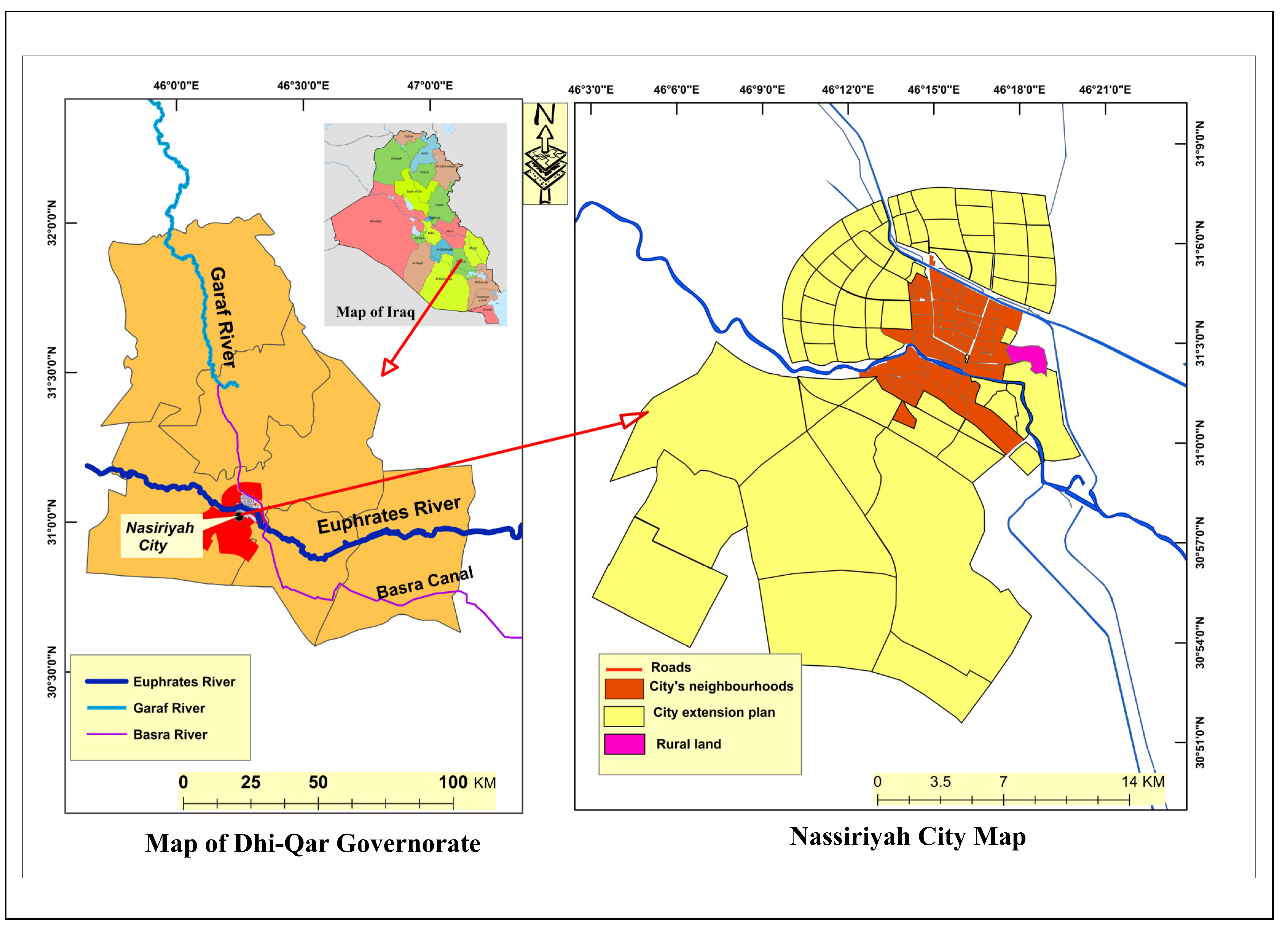
2.1. Study Area
2.2. Criteria Selection
2.2.1. Unmet Demand (C1)
2.2.2. Proximity to the River Basin (C2)
2.2.3. Proximity to PS (C3)
2.2.4. Proximity to Major Pipes (C4)
2.2.5. Age of the Network Pipes (C5)
2.2.6. Capacity of Reservoir (C6)
2.2.7. Electricity Supply (C7)
2.2.8. Population (C8)
2.2.9. Population Density (C9)
2.2.10. Unemployment Ratio (C10)
2.3. Data Collection
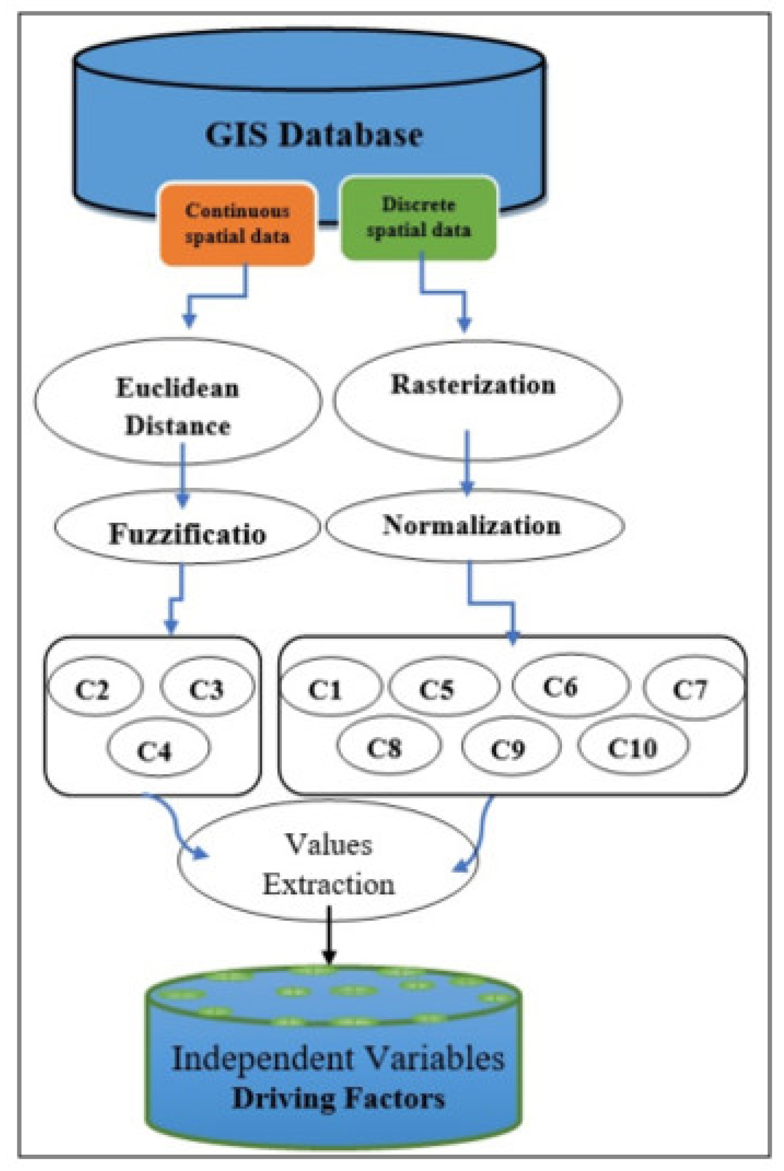
2.4. Generating Driving Factors
2.4.1. Euclidean Distance and Rasterization
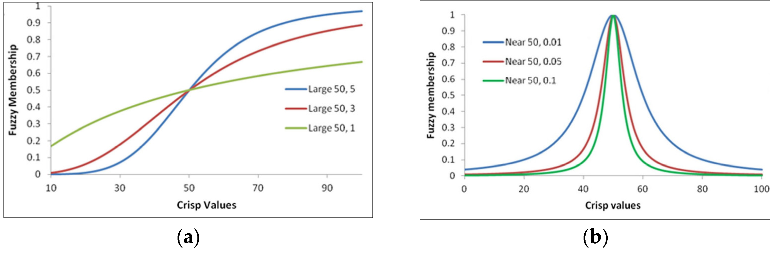
2.4.2. Fuzzy Large and Near Membership
2.5. Public Participation Process
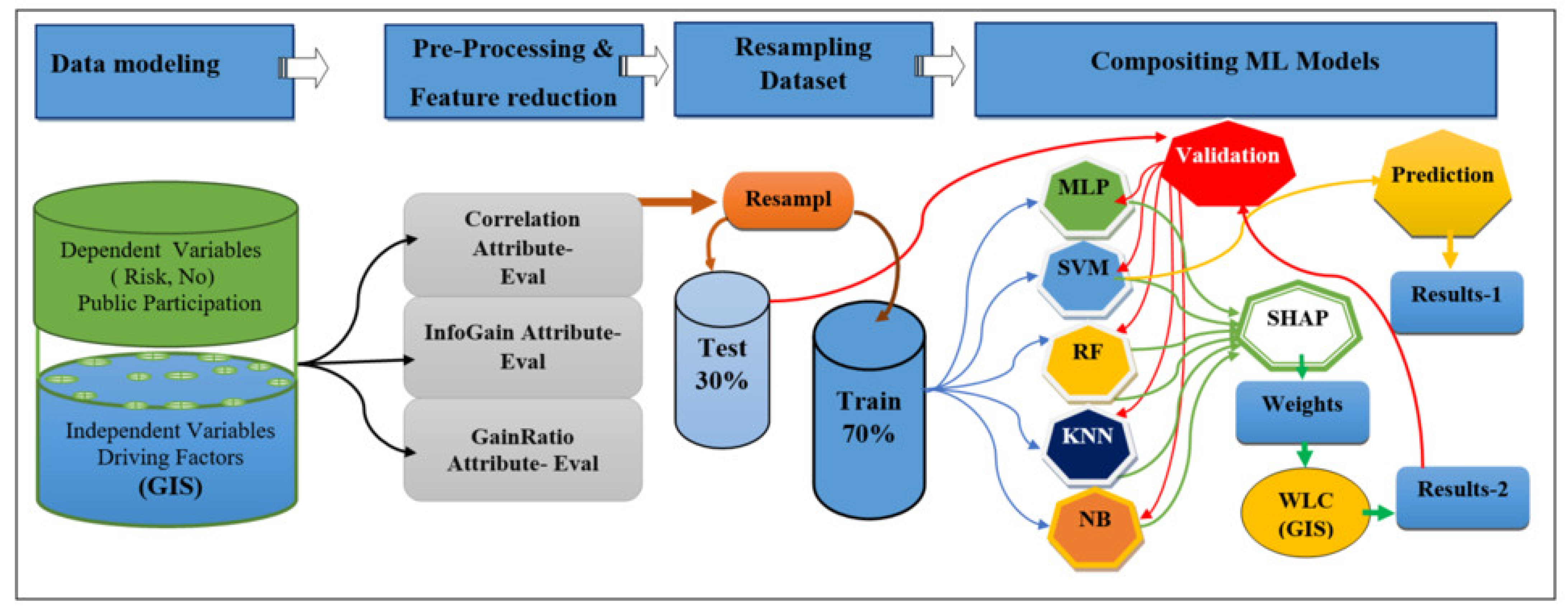
2.6. Data Model in ML
2.7. Constructing ML Models
2.7.1. Feature Reduction Using Weka Software
2.7.2. Modelling with Orange Software Application
2.8. Model Validation
2.9. Production of WSR Maps Using GIS
3. Results
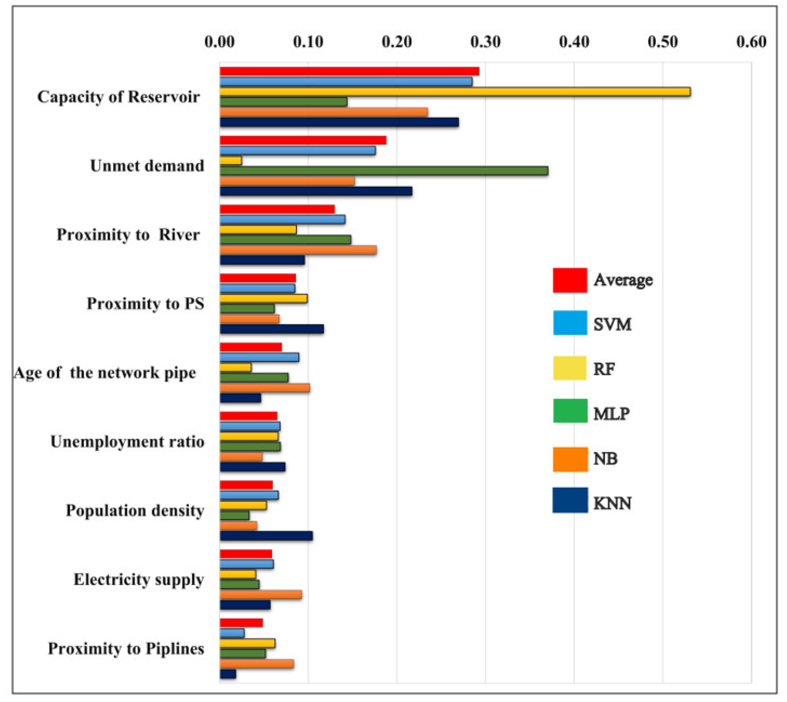
3.1. Results of Feature Reduction
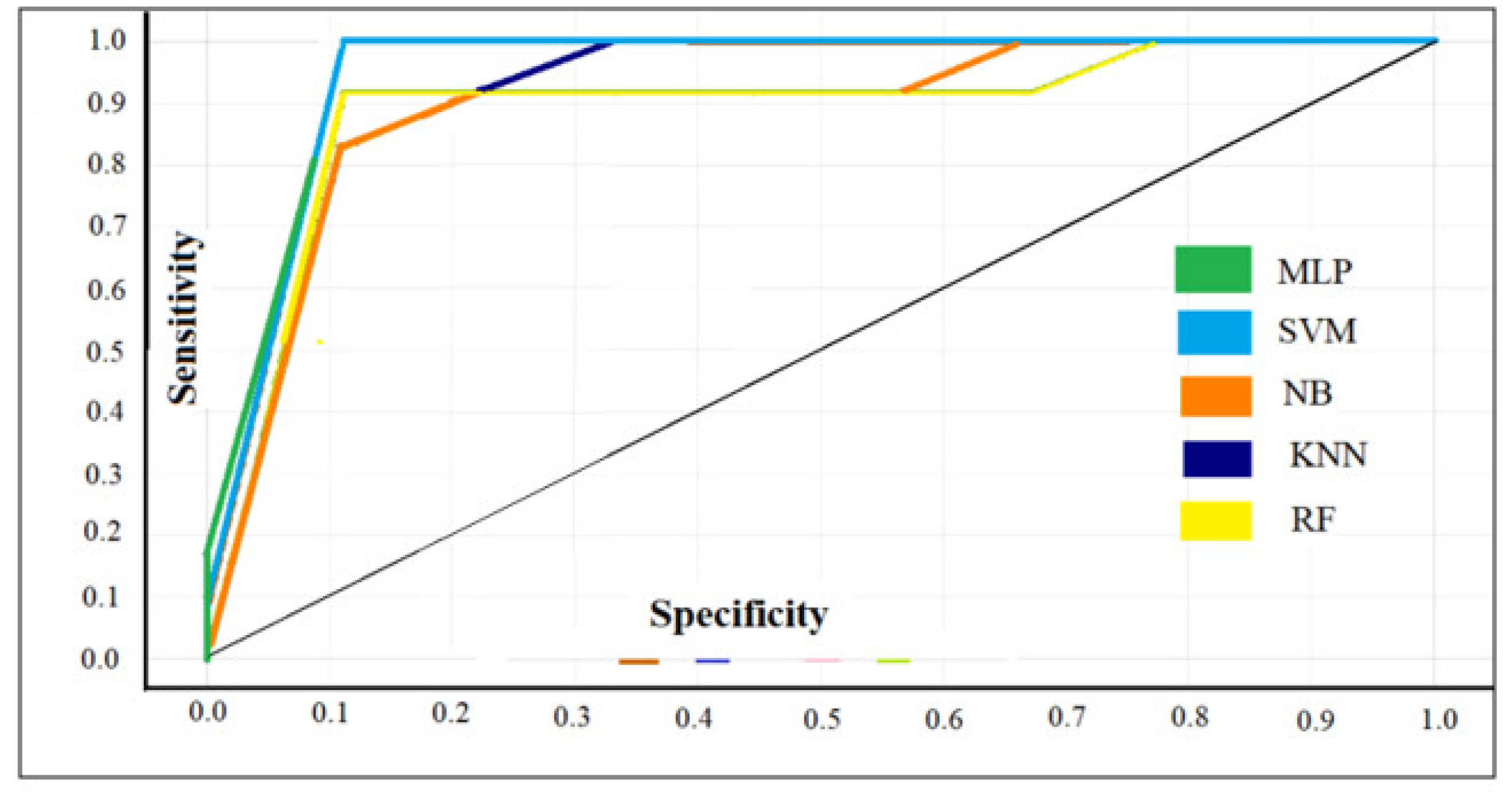
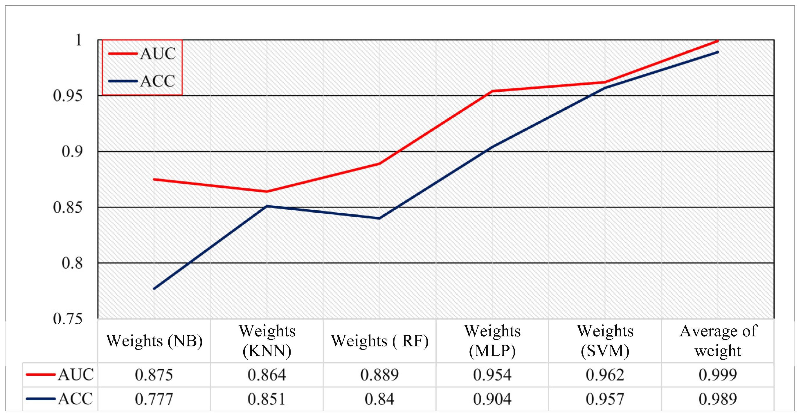
3.2. Performance of ML Models
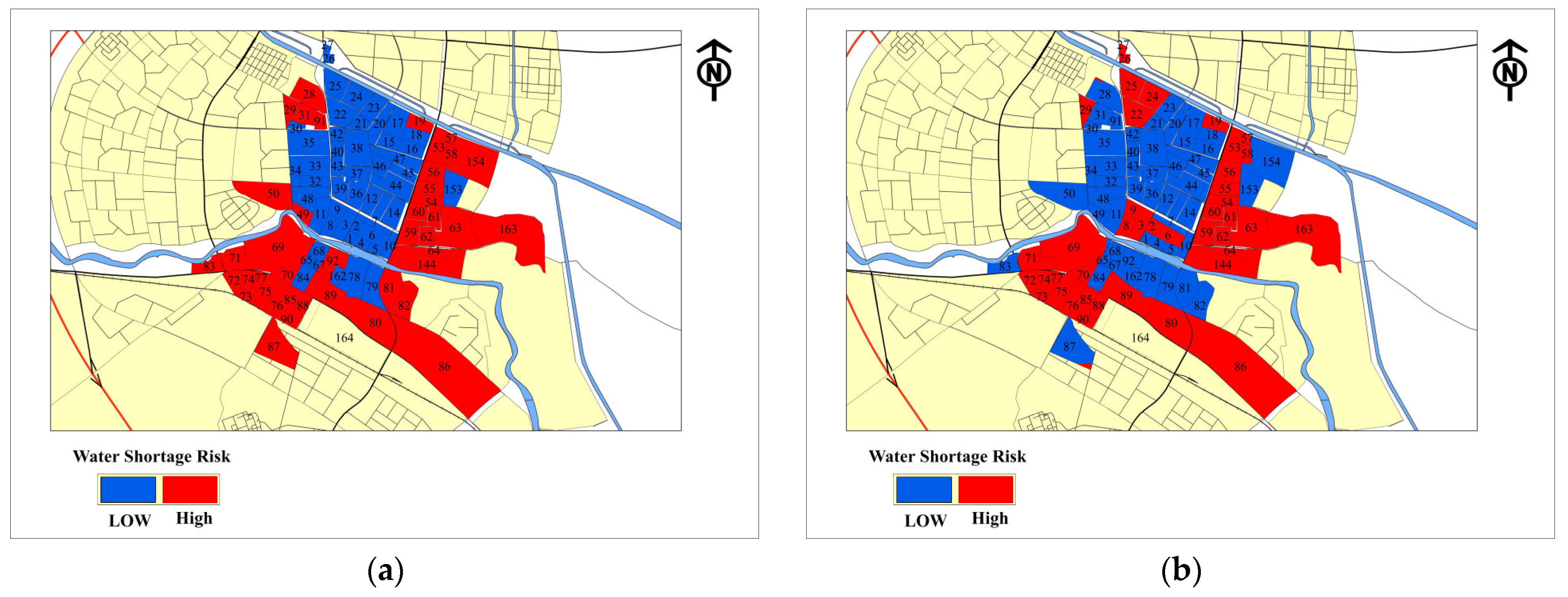
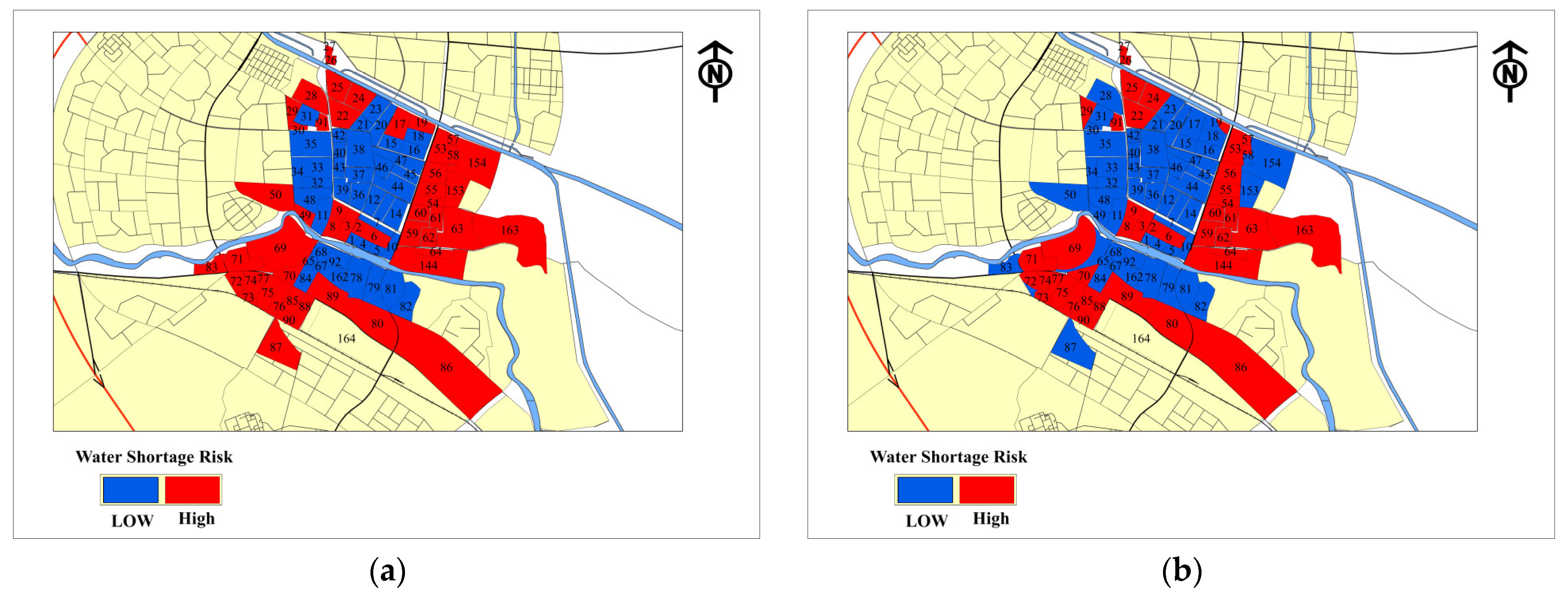
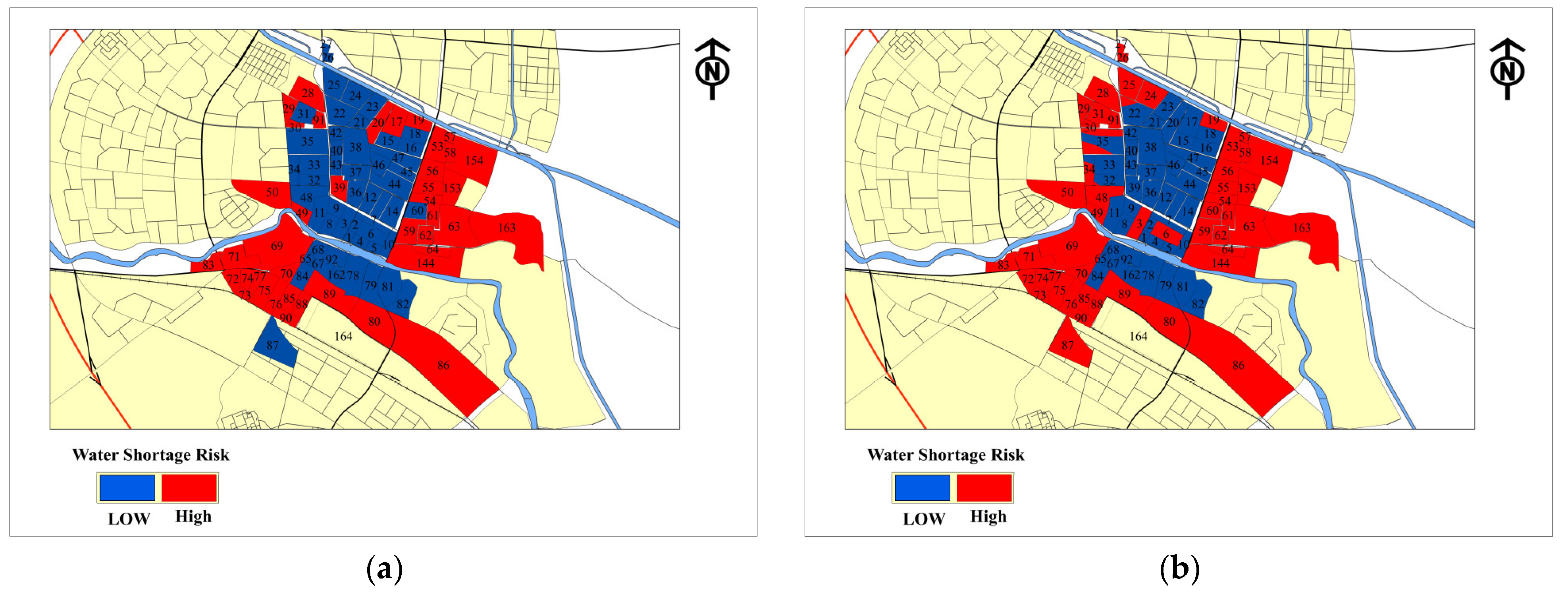
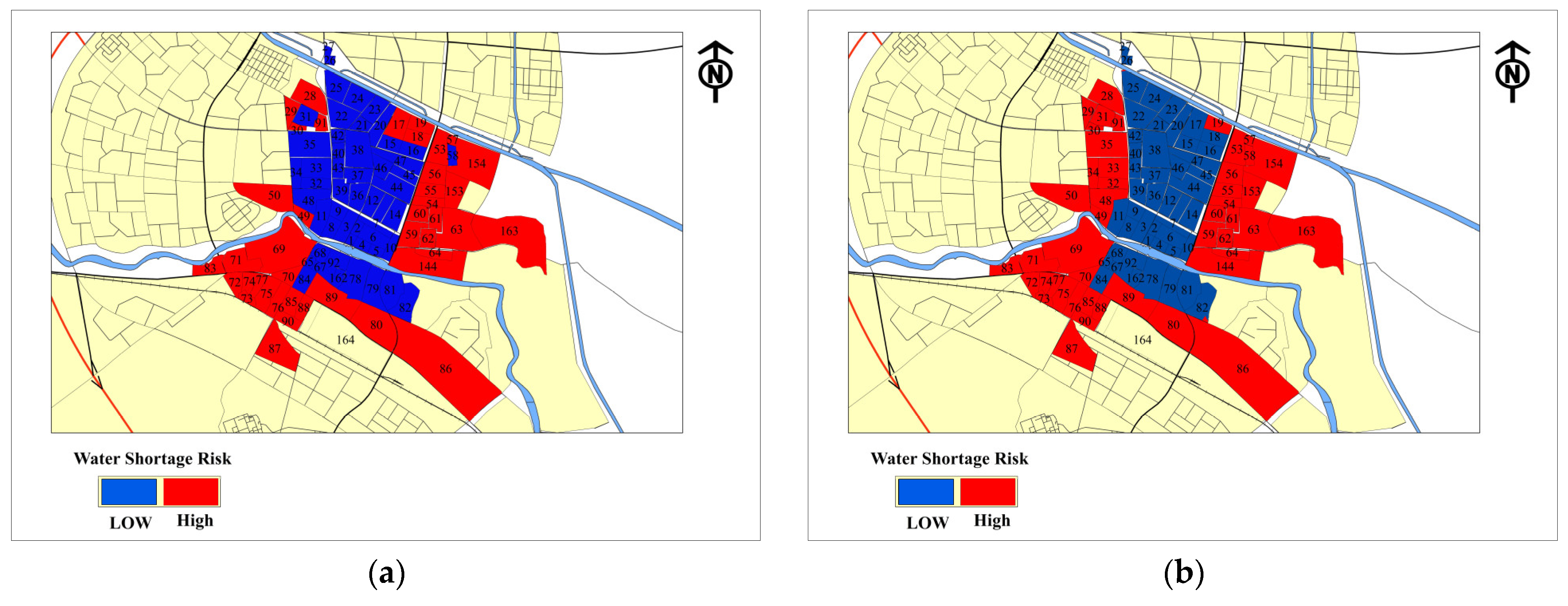
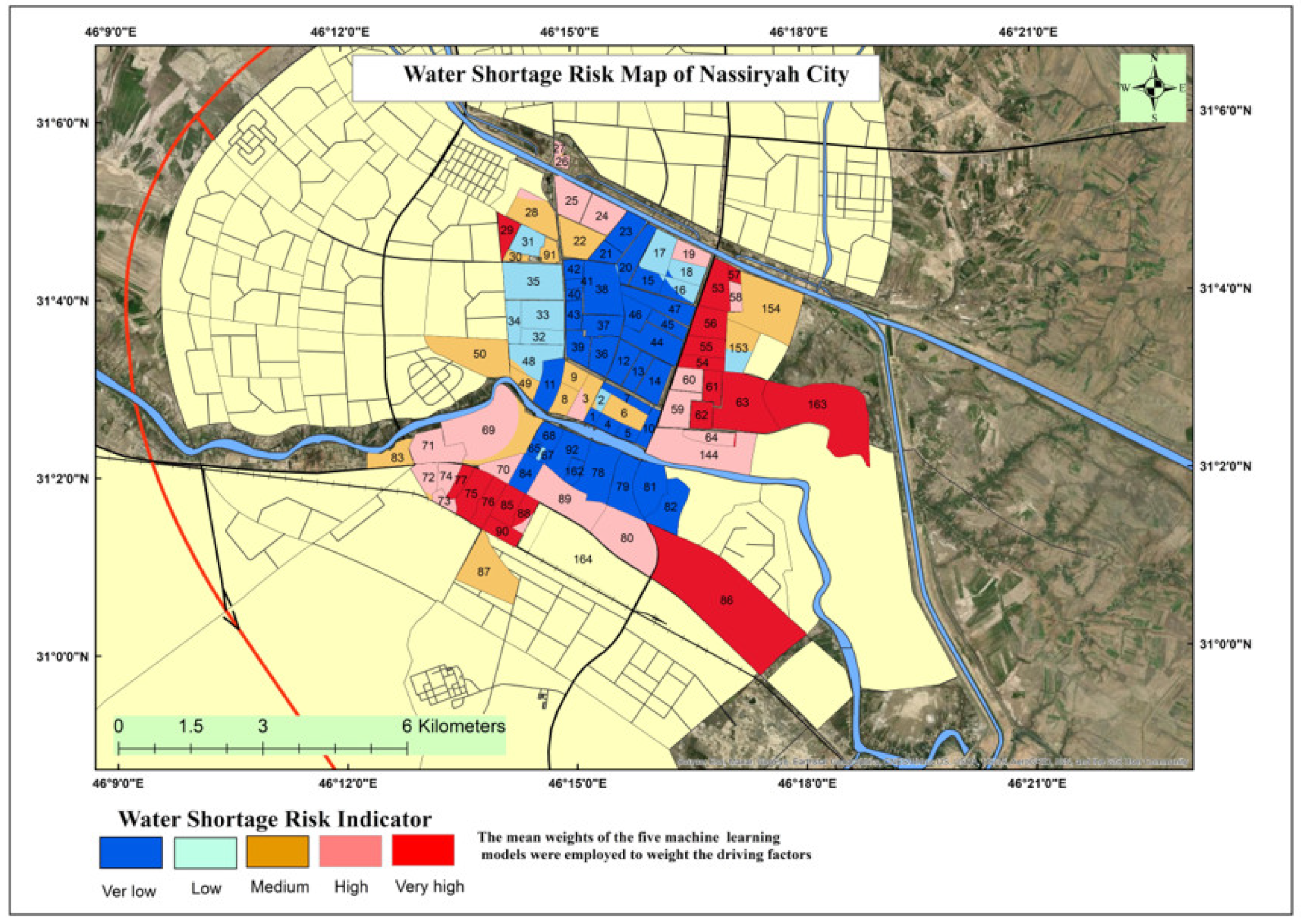
3.3. GIS Techniques Results
4. Validation
5. Discussion
6. Conclusions
Author Contributions
Funding
Institutional Review Board Statement
Informed Consent Statement
Data Availability Statement
Conflicts of Interest
References
- Johannessen, O.M.; Shalina, E.V. Population increase impacts the climate, using the sensitive Arctic as an example. Atmospheric Ocean. Sci. Lett. 2022, 15, 100192. [Google Scholar] [CrossRef]
- Gesualdo, G.C.; Sone, J.S.; Galvão, C.D.O.; Martins, E.S.; Montenegro, S.M.G.L.; Tomasella, J.; Mendiondo, E.M. Unveiling water security in Brazil: Current challenges and future perspectives. Hydrol. Sci. J. 2021, 66, 759–768. [Google Scholar] [CrossRef]
- Ahmadi, M.S.; Sušnik, J.; Veerbeek, W.; Zevenbergen, C. Towards a global day zero? Assessment of current and future water supply and demand in 12 rapidly developing megacities. Sustain. Cities Soc. 2020, 61, 102295. [Google Scholar] [CrossRef]
- Luo, P.; Sun, Y.; Wang, S.; Wang, S.; Lyu, J.; Zhou, M.; Nakagami, K.; Takara, K.; Nover, D. Historical assessment and future sustainability challenges of Egyptian water resources management. J. Clean. Prod. 2020, 263, 121154. [Google Scholar] [CrossRef]
- Rafiei, F.; Gharechelou, S.; Golian, S.; Johnson, B.A. Aquifer and Land Subsidence Interaction Assessment Using Sentinel-1 Data and DInSAR Technique. ISPRS Int. J. Geo-Inf. 2022, 11, 495. [Google Scholar] [CrossRef]
- Albarqouni, M.M.Y.; Yagmur, N.; Balcik, F.B.; Sekertekin, A. Assessment of Spatio-Temporal Changes in Water Surface Extents and Lake Surface Temperatures Using Google Earth Engine for Lakes Region, Türkiye. ISPRS Int. J. Geo-Inf. 2022, 11, 407. [Google Scholar] [CrossRef]
- Hanoon, S.K.; Abdullah, A.F.; Shafri, H.Z.M.; Wayayok, A. Using Supervised Classification technique to monitor hydrological systems of Mesopotamia marshes in Dhi-Qar province (Iraq). In Proceedings of the IGARSS 2022—2022 IEEE International Geoscience and Remote Sensing Symposium, Kuala Lumpur, Malaysia, 17–22 July 2022; pp. 6189–6192. [Google Scholar]
- Chapagain, K.; Aboelnga, H.T.; Babel, M.S.; Ribbe, L.; Shinde, V.R.; Sharma, D.; Dang, N.M. Urban water security: A comparative assessment and policy analysis of five cities in diverse developing countries of Asia. Environ. Dev. 2022, 43, 100713. [Google Scholar] [CrossRef]
- Asghar, A.; Iqbal, J.; Amin, A.; Ribbe, L. Integrated hydrological modeling for assessment of water demand and supply under socio-economic and IPCC climate change scenarios using WEAP in Central Indus Basin. J. Water Supply Res. Technol. 2019, 68, 136–148. [Google Scholar] [CrossRef]
- Yousuf, M.A.; Rapantova, N.; Younis, J.H. Sustainable Water Management in Iraq (Kurdistan) as a Challenge for Governmental Responsibility. Water 2018, 10, 1651. [Google Scholar] [CrossRef]
- Ougougdal, H.A.; Khebiza, M.Y.; Messouli, M.; Lachir, A. Assessment of futurewater demand and supply under IPCC climate change and socio-economic scenarios, using a combination of models in Ourika watershed, High Atlas, Morocco. Water 2020, 12, 1751. [Google Scholar] [CrossRef]
- Amin, A.; Iqbal, J.; Asghar, A.; Ribbe, L. Analysis of current and futurewater demands in the Upper Indus Basin under IPCC climate and socio-economic scenarios using a hydro-economic WEAP Model. Water 2018, 10, 537. [Google Scholar] [CrossRef]
- Alwan, I.A.; Aziz, N.A.; Hamoodi, M.N. Potential Water Harvesting Sites Identification Using Spatial Multi-Criteria Evaluation in Maysan Province, Iraq. ISPRS Int. J. Geo-Inf. 2020, 9, 235. [Google Scholar] [CrossRef]
- de Sousa Cordão, M.J.; Rufino, I.A.A.; Barros Ramalho Alves, P.; Barros Filho, M.N.M. Water shortage risk mapping: A GIS-MCDA approach for a medium-sized city in the Brazilian semi-arid region. Urban Water J. 2020, 17, 642–655. [Google Scholar] [CrossRef]
- Al-Juaidi, A.E.; Al-Shotairy, A.S. Evaluation of municipal water supply system options using water evaluation and planning system (WEAP): Jeddah case study. Desalination Water Treat. 2020, 176, 317–323. [Google Scholar] [CrossRef]
- Chini, C.M.; Stillwell, A.S. One Model Does Not Fit All: Bottom-Up Indicators of Residential Water Use Provide Limited Explanation of Urban Water Fluxes. J. Sustain. Water Built Environ. 2020, 6, 04020011. [Google Scholar] [CrossRef]
- Rufino, I.; Djordjević, S.; de Brito, H.C.; Alves, P.B.R. Multi-temporal built-up grids of brazilian cities: How trends and dynamic modelling could help on resilience challenges? Sustainability 2021, 13, 748. [Google Scholar] [CrossRef]
- Khosravi, K.; Shahabi, H.; Pham, B.T.; Adamowski, J.; Shirzadi, A.; Pradhan, B.; Dou, J.; Ly, H.-B.; Gróf, G.; Ho, H.L.; et al. A comparative assessment of flood susceptibility modeling using Multi-Criteria Decision-Making Analysis and Machine Learning Methods. J. Hydrol. 2019, 573, 311–323. [Google Scholar] [CrossRef]
- Sachit, M.S.; Shafri, H.Z.M.; Abdullah, A.F.; Rafie, A.S.M.; Gibril, M.B.A. Global Spatial Suitability Mapping of Wind and Solar Systems Using an Explainable AI-Based Approach. ISPRS Int. J. Geo-Inf. 2022, 11, 422. [Google Scholar] [CrossRef]
- Martyn, K.; Kadziński, M. Deep preference learning for multiple criteria decision analysis. Eur. J. Oper. Res. 2023, 305, 781–805. [Google Scholar] [CrossRef]
- Roy, A.; Kar, B. A multicriteria decision analysis framework to measure equitable healthcare access during COVID-19. J. Transp. Heal. 2022, 24, 101331. [Google Scholar] [CrossRef]
- Hanoon, S.K.; Abdullah, A.F.; Shafri, H.Z.M.; Wayayok, A. Using scenario modelling for adapting to urbanization and water scarcity: Towards a sustainable city in semi-arid areas. Period. Eng. Nat. Sci. (PEN) 2021, 10, 518–532. [Google Scholar] [CrossRef]
- Almansi, K.Y.; Shariff, A.R.M.; Abdullah, A.F.; Ismail, S.N.S. Hospital Site Assessment Using Three Machine Learning Approaches: Evidence from the Gaza Strip in Palestine. Appl. Sci. 2021, 11, 11054. [Google Scholar] [CrossRef]
- Kumar, P.; Sharma, R.; Bhaumik, S. MCDA techniques used in optimization of weights and ratings of DRASTIC model for groundwater vulnerability assessment. Data Sci. Manag. 2022, 5, 28–41. [Google Scholar] [CrossRef]
- Nachappa, T.G.; Piralilou, S.T.; Gholamnia, K.; Ghorbanzadeh, O.; Rahmati, O.; Blaschke, T. Flood susceptibility mapping with machine learning, multi-criteria decision analysis and ensemble using Dempster Shafer Theory. J. Hydrol. 2020, 590, 125275. [Google Scholar] [CrossRef]
- Iban, M.C.; Sekertekin, A. Machine learning based wildfire susceptibility mapping using remotely sensed fire data and GIS: A case study of Adana and Mersin provinces, Turkey. Ecol. Inform. 2022, 69, 101647. [Google Scholar] [CrossRef]
- Wang, S.; Peng, H.; Hu, Q.; Jiang, M. Analysis of runoff generation driving factors based on hydrological model and interpretable machine learning method. J. Hydrol. Reg. Stud. 2022, 42, 101139. [Google Scholar] [CrossRef]
- Haltofova, B. Using Crowdsourcing To Support Civic Engagement in Strategic Urban Development Planning: A Case Study of Ostrava, Czech Republic. J. Competitiveness 2018, 10, 85–103. [Google Scholar] [CrossRef]
- Aubert, A.H.; Esculier, F.; Lienert, J. Recommendations for online elicitation of swing weights from citizens in environmental decision-making. Oper. Res. Perspect. 2020, 7, 100156. [Google Scholar] [CrossRef]
- Bugs, G.; Granell, C.; Fonts, O.; Huerta, J.; Painho, M. An assessment of Public Participation GIS and Web 2.0 technologies in urban planning practice in Canela, Brazil. Cities 2010, 27, 172–181. [Google Scholar] [CrossRef]
- Li, W.; Shi, Y.; Huang, F.; Hong, H.; Song, G. Uncertainties of Collapse Susceptibility Prediction Based on Remote Sensing and GIS: Effects of Different Machine Learning Models. Front. Earth Sci. 2021, 9, 731058. [Google Scholar] [CrossRef]
- Sachit, M.S.; Shafri, H.Z.M.; Abdullah, A.F.; Rafie, A.S.M. Combining Re-Analyzed Climate Data and Landcover Products to Assess the Temporal Complementarity of Wind and Solar Resources in Iraq. Sustainability 2022, 14, 388. [Google Scholar] [CrossRef]
- Millington, N. Producing water scarcity in São Paulo, Brazil: The 2014-2015 water crisis and the binding politics of infrastructure. Politi-Geogr. 2018, 65, 26–34. [Google Scholar] [CrossRef]
- Simukonda, K.; Farmani, R.; Butler, D. Intermittent water supply systems: Causal factors, problems and solution options. Urban Water J. 2018, 15, 488–500. [Google Scholar] [CrossRef]
- Noori, A.; Bonakdari, H.; Hassaninia, M.; Morovati, K.; Khorshidi, I.; Noori, A.; Gharabaghi, B. A reliable GIS-based FAHP-FTOPSIS model to prioritize urban water supply management scenarios: A case study in semi-arid climate. Sustain. Cities Soc. 2022, 81, 103846. [Google Scholar] [CrossRef]
- Krueger, E.H.; Rao, P.S.C.; Borchardt, D. Quantifying urban water supply security under global change. Glob. Environ. Chang. 2019, 56, 66–74. [Google Scholar] [CrossRef]
- Liu, Y.; Tan, Q.; Zhang, X.; Han, J.; Guo, M. How does electricity supply mode affect energy-water-emissions nexus in urban energy system? Evidence from energy transformation in Beijing, China. J. Clean. Prod. 2022, 366, 132892. [Google Scholar] [CrossRef]
- Dallison, R.J.; Patil, S.D.; Williams, A.P. Impacts of climate change on future water availability for hydropower and public water supply in Wales, UK. J. Hydrol. Reg. Stud. 2021, 36, 100866. [Google Scholar] [CrossRef]
- Mena, D.; Solera, A.; Restrepo, L.; Pimiento, M.; Cañón, M.; Duarte, F. An analysis of unmet water demand under climate change scenarios in the Gualí river basin, Colombia, through the implementation of hydro-bid and weap hydrological modeling tools. J. Water Clim. Chang. 2021, 12, 185–200. [Google Scholar] [CrossRef]
- Savari, M.; Mombeni, A.S.; Izadi, H. Socio-psychological determinants of Iranian rural households’ adoption of water consumption curtailment behaviors. Sci. Rep. 2022, 12, 1–12. [Google Scholar] [CrossRef]
- Wee, S.Y.; Aris, A.Z.; Yusoff, F.M.; Praveena, S.M.; Harun, R. Drinking water consumption and association between actual and perceived risks of endocrine disrupting compounds. npj Clean Water 2022, 5, 1–10. [Google Scholar] [CrossRef]
- Zhuang, J.; Sela, L. Impact of Emerging Water Savings Scenarios on Performance of Urban Water Networks. J. Water Resour. Plan. Manag. 2020, 146, 04019063. [Google Scholar] [CrossRef]
- Eryiğit, M.; Sulaiman, S.O. Specifying optimum water resources based on cost-benefit relationship for settlements by artificial immune systems: Case study of Rutba City, Iraq. Water Supply 2022, 22, 5873–5881. [Google Scholar] [CrossRef]
- Vicente, D.J.; Garrote, L.; Sánchez, R.; Santillán, D. Pressure Management in Water Distribution Systems: Current Status, Proposals, and Future Trends. J. Water Resour. Plan. Manag. 2016, 142, 04015061. [Google Scholar] [CrossRef]
- Zyoud, S.H.; Kaufmann, L.G.; Shaheen, H.; Samhan, S.; Fuchs-Hanusch, D. A framework for water loss management in developing countries under fuzzy environment: Integration of Fuzzy AHP with Fuzzy TOPSIS. Expert Syst. Appl. 2016, 61, 86–105. [Google Scholar] [CrossRef]
- Hashemi, S.; Filion, Y.; Speight, V.; Long, A. Effect of Pipe Size and Location on Water-Main Head Loss in Water Distribution Systems. J. Water Resour. Plan. Manag. 2020, 146, 06020006. [Google Scholar] [CrossRef]
- Latif, J.; Shakir, M.Z.; Edwards, N.; Jaszczykowski, M.; Ramzan, N.; Edwards, V. Review on condition monitoring techniques for water pipelines. Measurement 2022, 193, 110895. [Google Scholar] [CrossRef]
- Zielina, M.; Bielski, A.; Młyńska, A. Leaching of chromium and lead from the cement mortar lining into the flowing drinking water shortly after pipeline rehabilitation. J. Clean. Prod. 2022, 362, 132512. [Google Scholar] [CrossRef]
- Moossa, B.; Trivedi, P.; Saleem, H.; Zaidi, S.J. Desalination in the GCC countries- a review. J. Clean. Prod. 2022, 357, 131717. [Google Scholar] [CrossRef]
- Pissarra, T.C.T.; Fernandes, L.F.S.; Pacheco, F.A.L. Production of clean water in agriculture headwater catchments: A model based on the payment for environmental services. Sci. Total Environ. 2021, 785, 147331. [Google Scholar] [CrossRef] [PubMed]
- Yan, X.; Jie, W.; Minjun, S.; Shouyang, W.; Zhuoying, Z. China’s regional imbalance in electricity demand, power and water pricing—From the perspective of electricity-related virtual water transmission. Energy 2022, 257, 42–50. [Google Scholar] [CrossRef]
- Bakhtiari, P.H.; Nikoo, M.R.; Izady, A.; Talebbeydokhti, N. A coupled agent-based risk-based optimization model for integrated urban water management. Sustain. Cities Soc. 2020, 53, 101922. [Google Scholar] [CrossRef]
- Wang, Z.-H.; von Gnechten, R.; Sampson, D.A.; White, D.D. Wastewater Reclamation Holds a Key for Water Sustainability in Future Urban Development of Phoenix Metropolitan Area. Sustainability 2019, 11, 3537. [Google Scholar] [CrossRef]
- Chandra, G.; Chakraborty, M.; Sinha, A. Framework for Assessing Efficient Water Consumption Attributes and Their Relative Importance in Office Complexes. Asian J. Water, Environ. Pollut. 2017, 14, 65–74. [Google Scholar] [CrossRef]
- Diao, K.; Sitzenfrei, R.; Rauch, W. The Impacts of Spatially Variable Demand Patterns on Water Distribution System Design and Operation. Water 2019, 11, 567. [Google Scholar] [CrossRef]
- Chen, X.; Li, F.; Li, X.; Hu, Y.; Hu, P. Evaluating and mapping water supply and demand for sustainable urban ecosystem management in Shenzhen, China. J. Clean. Prod. 2019, 251, 119754. [Google Scholar] [CrossRef]
- Van Leeuwen, C.J. Water governance and the quality of water services in the city of Melbourne. Urban Water J. 2017, 14, 247–254. [Google Scholar] [CrossRef]
- Valencia, A.; Qiu, J.; Chang, N.-B. Integrating sustainability indicators and governance structures via clustering analysis and multicriteria decision making for an urban agriculture network. Ecol. Indic. 2022, 142, 109237. [Google Scholar] [CrossRef]
- Kuntiyawichai, K.; Wongsasri, S. Assessment of Drought Severity and Vulnerability in the Lam Phaniang River Basin, Thailand. Water 2021, 13, 2743. [Google Scholar] [CrossRef]
- Wang, L.; Jin, G.; Xiong, X.; Zhang, H.; Wu, K. Object-Based Automatic Mapping of Winter Wheat Based on Temporal Phenology Patterns Derived from Multitemporal Sentinel-1 and Sentinel-2 Imagery. ISPRS Int. J. Geo-Inf. 2022, 11, 424. [Google Scholar] [CrossRef]
- Oliver, M.A.; Webster, R. Kriging: A method of interpolation for geographical information systems. Int. J. Geogr. Inf. Syst. 1990, 4, 312–332. [Google Scholar] [CrossRef]
- Li, Z.; Chen, H.; Yan, W. Exploring Spatial Distribution of Urban Park Service Areas in Shanghai Based on Travel Time Estimation: A Method Combining Multi-Source Data. ISPRS Int. J. Geo-Inf. 2021, 10, 608. [Google Scholar] [CrossRef]
- Baalousha, H.; Tawabini, B.; Seers, T. Fuzzy or Non-Fuzzy? A Comparison between Fuzzy Logic-Based Vulnerability Mapping and DRASTIC Approach Using a Numerical Model. A Case Study from Qatar. Water 2021, 13, 1288. [Google Scholar] [CrossRef]
- Arab, S.T.; Ahamed, T. Land Suitability Analysis for Potential Vineyards Extension in Afghanistan at Regional Scale Using Remote Sensing Datasets. Remote Sens. 2022, 14, 4450. [Google Scholar] [CrossRef]
- Liu, J.; Li, Y.; Xiao, B.; Jiao, J. Coupling Fuzzy Multi-Criteria Decision-Making and Clustering Algorithm for MSW Landfill Site Selection (Case Study: Lanzhou, China). ISPRS Int. J. Geo-Inf. 2021, 10, 403. [Google Scholar] [CrossRef]
- Kritikos, T.; Davies, T. Assessment of rainfall-generated shallow landslide/debris-flow susceptibility and runout using a GIS-based approach: Application to western Southern Alps of New Zealand. Landslides 2015, 12, 1051–1075. [Google Scholar] [CrossRef]
- Rahman, M.; Szabó, G. Sustainable Urban Land-Use Optimization Using GIS-Based Multicriteria Decision-Making (GIS-MCDM) Approach. ISPRS Int. J. Geo-Inf. 2022, 11, 313. [Google Scholar] [CrossRef]
- Salvati, P.; Ardizzone, F.; Cardinali, M.; Fiorucci, F.; Fugnoli, F.; Guzzetti, F.; Marchesini, I.; Rinaldi, G.; Rossi, M.; Santangelo, M.; et al. Acquiring vulnerability indicators to geo-hydrological hazards: An example of mobile phone-based data collection. Int. J. Disaster Risk Reduct. 2021, 55, 102087. [Google Scholar] [CrossRef]
- Chou, J.-S.; Truong, D.-N.; Tsai, C.-F. Solving Regression Problems with Intelligent Machine Learner for Engineering Informatics. Mathematics 2021, 9, 686. [Google Scholar] [CrossRef]
- Güneş, S.S.; Yeşil, Ç.; Gurdal, E.E.; Korkmaz, E.E.; Yarım, M.; Aydın, A.; Sipahi, H. Primum non nocere: In silico prediction of adverse drug reactions of antidepressant drugs. Comput. Toxicol. 2021, 18, 100165. [Google Scholar] [CrossRef]
- Gao, W.; Alsarraf, J.; Moayedi, H.; Shahsavar, A.; Nguyen, H. Comprehensive preference learning and feature validity for designing energy-efficient residential buildings using machine learning paradigms. Appl. Soft Comput. 2019, 84, 105748. [Google Scholar] [CrossRef]
- Albagmi, F.M.; Alansari, A.; Al Shawan, D.S.; AlNujaidi, H.Y.; Olatunji, S.O. Prediction of generalized anxiety levels during the Covid-19 pandemic: A machine learning-based modeling approach. Inform. Med. Unlocked 2022, 28, 100854. [Google Scholar] [CrossRef] [PubMed]
- Sindhu, S.S.S.; Geetha, S.; Kannan, A. Decision tree based light weight intrusion detection using a wrapper approach. Expert Syst. Appl. 2012, 39, 129–141. [Google Scholar] [CrossRef]
- Amirruddin, A.D.; Muharam, F.M.; Ismail, M.H.; Tan, N.P. Synthetic Minority Over-sampling TEchnique (SMOTE) and Logistic Model Tree (LMT)-Adaptive Boosting algorithms for classifying imbalanced datasets of nutrient and chlorophyll sufficiency levels of oil palm (Elaeis guineensis) using spectroradiometers and unmanned aerial vehicles. Comput. Electron. Agric. 2022, 193, 106646. [Google Scholar] [CrossRef]
- Otchere, D.A.; Ganat, T.O.A.; Gholami, R.; Ridha, S. Application of supervised machine learning paradigms in the prediction of petroleum reservoir properties: Comparative analysis of ANN and SVM models. J. Pet. Sci. Eng. 2021, 200, 108182. [Google Scholar] [CrossRef]
- Almeida, V.G.; Vieira, J.; Santos, P.; Pereira, T.; Pereira, H.C.; Correia, C.; Pego, M.; Cardoso, J. Machine Learning Techniques for Arterial Pressure Waveform Analysis. J. Pers. Med. 2013, 3, 82–101. [Google Scholar] [CrossRef] [PubMed]
- Nguyen, D.D.; Roussis, P.C.; Pham, B.T.; Ferentinou, M.; Mamou, A.; Vu, D.Q.; Bui, Q.-A.T.; Trong, D.K.; Asteris, P.G. Bagging and Multilayer Perceptron Hybrid Intelligence Models Predicting the Swelling Potential of Soil. Transp. Geotech. 2022, 36, 100797. [Google Scholar] [CrossRef]
- Bansal, D.; Chhikara, R.; Khanna, K.; Gupta, P. Comparative Analysis of Various Machine Learning Algorithms for Detecting Dementia. Procedia Comput. Sci. 2018, 132, 1497–1502. [Google Scholar] [CrossRef]
- Ajdadi, F.R.; Gilandeh, Y.A.; Mollazade, K.; Hasanzadeh, R.P. Application of machine vision for classification of soil aggregate size. Soil Tillage Res. 2016, 162, 8–17. [Google Scholar] [CrossRef]
- Zarei, R.; He, J.; Siuly, S.; Zhang, Y. A PCA aided cross-covariance scheme for discriminative feature extraction from EEG signals. Comput. Methods Programs Biomed. 2017, 146, 47–57. [Google Scholar] [CrossRef]
- Azoff, E.M. Reducing error in neural network time series forecasting. Neural Comput. Appl. 1993, 1, 240–247. [Google Scholar] [CrossRef]
- Mehmood, Z.; Asghar, S. Customizing SVM as a base learner with AdaBoost ensemble to learn from multi-class problems: A hybrid approach AdaBoost-MSVM. Knowl.-Based Syst. 2021, 217, 106845. [Google Scholar] [CrossRef]
- Güven, I.; Şimşir, F. Demand forecasting with color parameter in retail apparel industry using artificial neural networks (ANN) and support vector machines (SVM) methods. Comput. Ind. Eng. 2020, 147, 106678. [Google Scholar] [CrossRef]
- Gâlmeanu, H.; Andonie, R. Weighted Incremental–Decremental Support Vector Machines for concept drift with shifting window. Neural Networks 2022, 152, 528–541. [Google Scholar] [CrossRef] [PubMed]
- Balaji, V.; Suganthi, S.; Rajadevi, R.; Kumar, V.K.; Balaji, B.S.; Pandiyan, S. Skin disease detection and segmentation using dynamic graph cut algorithm and classification through Naive Bayes classifier. Measurement 2020, 163, 107922. [Google Scholar] [CrossRef]
- Yao, J.; Ye, Y. The effect of image recognition traffic prediction method under deep learning and naive Bayes algorithm on freeway traffic safety. Image Vis. Comput. 2020, 103, 103971. [Google Scholar] [CrossRef]
- Sun, X.; Opulencia, M.J.C.; Alexandrovich, T.P.; Khan, A.; Algarni, M.; Abdelrahman, A. Modeling and optimization of vegetable oil biodiesel production with heterogeneous nano catalytic process: Multi-layer perceptron, decision regression tree, and K-Nearest Neighbor methods. Environ. Technol. Innov. 2022, 27, 102794. [Google Scholar] [CrossRef]
- Gou, J.; Sun, L.; Du, L.; Ma, H.; Xiong, T.; Ou, W.; Zhan, Y. A representation coefficient-based k-nearest centroid neighbor classifier. Expert Syst. Appl. 2022, 194, 116529. [Google Scholar] [CrossRef]
- Feng, T.; Wang, C.; Zhang, J.; Wang, B.; Jin, Y.-F. An improved artificial bee colony-random forest (IABC-RF) model for predicting the tunnel deformation due to an adjacent foundation pit excavation. Undergr. Space 2022, 7, 514–527. [Google Scholar] [CrossRef]
- Dai, Y.; Wang, Y.; Leng, M.; Yang, X.; Zhou, Q. LOWESS smoothing and Random Forest based GRU model: A short-term photovoltaic power generation forecasting method. Energy 2022, 256, 124661. [Google Scholar] [CrossRef]
- Yagoub, M.M.; Tesfaldet, Y.T.; Elmubarak, M.G.; Al Hosani, N. Extraction of Urban Quality of Life Indicators Using Remote Sensing and Machine Learning: The Case of Al Ain City, United Arab Emirates (UAE). ISPRS Int. J. Geo-Inf. 2022, 11, 458. [Google Scholar] [CrossRef]
- Onah, J.O.; Abdulhamid, S.M.; Abdullahi, M.; Hassan, I.H.; Al-Ghusham, A. Genetic Algorithm based feature selection and Naïve Bayes for anomaly detection in fog computing environment. Mach. Learn. Appl. 2021, 6, 100156. [Google Scholar] [CrossRef]
- Kordnoori, S.; Mostafaei, H.; Rostamy-Malkhalifeh, M.; Ostadrahimi, M. Diagnosis of Heart Disease Using Feature Selection Methods Based on Recurrent Fuzzy Neural Networks. IPTEK J. Technol. Sci. 2021, 32, 64. [Google Scholar] [CrossRef]
- Hashem, A.; Awad, A.; Shousha, H.; Alakel, W.; Salama, A.; Awad, T.; Mabrouk, M. Validation of a machine learning approach using FIB-4 and APRI scores assessed by the metavir scoring system: A cohort study. Arab J. Gastroenterol. 2021, 22, 88–92. [Google Scholar] [CrossRef]
- Lee, D.-H.; Kim, Y.-T.; Lee, S.-R. Shallow Landslide Susceptibility Models Based on Artificial Neural Networks Considering the Factor Selection Method and Various Non-Linear Activation Functions. Remote Sens. 2020, 12, 1194. [Google Scholar] [CrossRef]
- Malczewski, J. GIS-based land-use suitability analysis: A critical overview. Prog. Plan. 2004, 62, 3–65. [Google Scholar] [CrossRef]
- Hanoon, S.K.; Abdullah, A.F.; Shafri, H.Z.M.; Wayayok, A. Comprehensive Vulnerability Assessment of Urban Areas Using an Integration of Fuzzy Logic Functions: Case Study of Nasiriyah City in South Iraq. Earth 2022, 3, 699–732. [Google Scholar] [CrossRef]


| No. | Data | Description | Source of Data | Data Accuracy |
|---|---|---|---|---|
| 1 | Sentinel 2 image, acquired on 14 November 2021 | The images were used to determine the catchment area of the Garaf River Basin and land cover classes | European Union’s Earth observation programme (https://scihub.copernicus.eu, (accessed on 5 December 2021)) | 10 m |
| 3 | Land use shapefiles (SHF) of streets, districts borders and class of land uses | Shapefiles were used to extract land use classes, neighbourhoods’ borders and street paths | Nasiriyah City Municipality, Iraq | 2 m |
| 4 | Shapefiles and raster for the WSS (2021) | Data were used to generate network pipeline paths and determine the pipeline diameters and locations of the reservoirs, WTP and PS | Dhi-Qar Water Directorate | 2 m |
| 4 | Master plan of Nasiriyah City | Shapefiles were used to validate neighbourhoods’ borders, streets paths, pipeline paths and land use | The Office of Urban Planning, Nasiriyah City, Iraq | 2 m |
| 7 | Statistical data on unemployment (2021) | Data were used to extract a conditional factor (C10) | Department of Statistics in Ministry of Planning | - |
| 8 | Population census (2021) | Data were used to extract two conditional factors (C8 and C9) | Department of Statistics in Ministry of Planning | - |
| 9 | Shapefiles of network river | The shapefiles were used to extract location demand nodes, gauge location, and Garaf River path and its branches | Ministry of Irrigation/Dhi-Qar (Iraq) | 5 m |
| 10 | Hydrological data (1990–2021) | Garaf River’s monthly discharge was used to model the WEAP, and hydrological parameters were used to estimate the conditional factor (C1) | Ministry of Irrigation/Dhi-Qar (Iraq) | ±5% |
| 11 | Climate data (1984–2021) | Climate data were required for the WEAP model | (NASA/POWER) website, (https://power.larc.nasa.gov, (accessed on 21 April 2022)). | - |
| 12 | Site surveying work using GPS | The survey was needed to check locations of PS, reservoirs data, pipeline paths, WTP, piping division, and gauges of rivers | Author | 1 m |
| No | Attributes | InfoGain AttributeEval | GainRatio AttributeEval | Correlation AttributeEval |
|---|---|---|---|---|
| 1 | Capacity of reservoir | 0.615 | 0.621 | 0.739 |
| 2 | Proximity to river | 0.339 | 0.346 | 0.641 |
| 3 | Unmet demand | 0.339 | 0.346 | 0.652 |
| 4 | Proximity to pipelines | 0.196 | 0.298 | 0.241 |
| 5 | Age of the network pipe | 0.258 | 0.193 | 0.283 |
| 6 | Electricity supply | 0.191 | 0.294 | 0.223 |
| 7 | Proximity to PS | 0.149 | 0.262 | 0.364 |
| 8 | Unemployment ratio | 0.011 | 0.024 | 0.312 |
| 9 | Population | 0 | 0 | 0.1 |
| 10 | Population density | 0 | 0 | 0.126 |
| Model | AUC | CA | F1 | Precision | Recall |
|---|---|---|---|---|---|
| NB | 0.875 | 0.777 | 0.747 | 0.738 | 0.756 |
| RF | 0.889 | 0.84 | 0.831 | 0.755 | 0.925 |
| KNN | 0.864 | 0.851 | 0.844 | 0.927 | 0.776 |
| MLP | 0.954 | 0.904 | 0.897 | 0.951 | 0.848 |
| SVM | 0.962 | 0.957 | 0.958 | 0.92 | 1 |
| Model | AUC | CA | F1 | Precision | Recall | Specificity |
|---|---|---|---|---|---|---|
| MLP | 0.940 | 0.923 | 0.917 | 0.917 | 0.917 | 0.929 |
| SVM | 0.934 | 0.923 | 0.917 | 0.917 | 0.917 | 0.929 |
| KNN | 0.9116 | 0.885 | 0.869 | 0.909 | 0.833 | 0.929 |
| RF | 0.893 | 0.923 | 0.917 | 0.917 | 0.917 | 0.929 |
| NB | 0.875 | 0.846 | 0.846 | 0.786 | 0.917 | 0.786 |
Publisher’s Note: MDPI stays neutral with regard to jurisdictional claims in published maps and institutional affiliations. |
© 2022 by the authors. Licensee MDPI, Basel, Switzerland. This article is an open access article distributed under the terms and conditions of the Creative Commons Attribution (CC BY) license (https://creativecommons.org/licenses/by/4.0/).
Share and Cite
Hanoon, S.K.; Abdullah, A.F.; Shafri, H.Z.M.; Wayayok, A. A Novel Approach Based on Machine Learning and Public Engagement to Predict Water-Scarcity Risk in Urban Areas. ISPRS Int. J. Geo-Inf. 2022, 11, 606. https://doi.org/10.3390/ijgi11120606
Hanoon SK, Abdullah AF, Shafri HZM, Wayayok A. A Novel Approach Based on Machine Learning and Public Engagement to Predict Water-Scarcity Risk in Urban Areas. ISPRS International Journal of Geo-Information. 2022; 11(12):606. https://doi.org/10.3390/ijgi11120606
Chicago/Turabian StyleHanoon, Sadeq Khaleefah, Ahmad Fikri Abdullah, Helmi Z. M. Shafri, and Aimrun Wayayok. 2022. "A Novel Approach Based on Machine Learning and Public Engagement to Predict Water-Scarcity Risk in Urban Areas" ISPRS International Journal of Geo-Information 11, no. 12: 606. https://doi.org/10.3390/ijgi11120606
APA StyleHanoon, S. K., Abdullah, A. F., Shafri, H. Z. M., & Wayayok, A. (2022). A Novel Approach Based on Machine Learning and Public Engagement to Predict Water-Scarcity Risk in Urban Areas. ISPRS International Journal of Geo-Information, 11(12), 606. https://doi.org/10.3390/ijgi11120606