Article

Interday Stability of Taxi Travel Flow in Urban Areas

1
Academy of Digital China (Fujian), Fuzhou University, Fuzhou 350108, China
2
Key Laboratory of Spatial Data Mining and Information Sharing of Ministry of Education, Fuzhou University, Fuzhou 350002, China
3
National Engineering Research Centre of Geospatial Information Technology, Fuzhou University, Fuzhou 350002, China
4
State Key Laboratory of Information Engineering in Surveying, Mapping, and Remote Sensing, Wuhan University, Wuhan 430079, China
*
Author to whom correspondence should be addressed.
ISPRS Int. J. Geo-Inf. 2022, 11(12), 590; https://doi.org/10.3390/ijgi11120590
Submission received: 22 September 2022 / Revised: 17 November 2022 / Accepted: 20 November 2022 / Published: 24 November 2022

Abstract

:
Taxi travel flow patterns and their interday stability play an important role in the planning of urban transportation and public service facilities. Existing studies pay little attention to the stability of the travel flow patterns between days, and it is difficult to consider the impact of dynamic changes in daily travel demand analysis when supporting related decision making. Taxi trajectory data have been widely used in urban taxi travel-pattern analysis. This paper uses the taxi datasets of Shenzhen and New York to analyze and compare the interday stability of the taxi travel spatial structure and the flow volume based on the improved Levenshtein algorithm and geographic flow theory. The results show that (1) interday differences in taxi travel flow are obvious in both spatial structure and flow volume, high-frequency origin–destination (OD) trips are relatively stable; (2) the ODs between the central urban area and surrounding areas exhibit high traffic volume and high interday stability, and the ODs starting or ending at an airport exhibit high traffic stability; (3) one week’s data can describe 86% of the overall travel structure and 84% of travel flow in Shenzhen, and one week’s New York data can describe 73% of travel structure and 76% of travel flow. There are differences in the travel patterns of people in different cities, and the representativeness of datasets in different cities will be different. These findings can help to better understand the outcomes of taxi travel patterns derived from a relatively short period of data to avoid potential misuse in related decision making.

1. Introduction

Taxi travel patterns are closely related to the urban spatial structure. Taxi travel patterns include the travel spatial structure and travel flow [1]. The travel spatial structure is the skeletal framework of the OD matrix, where the skeleton is expressed as the connectivity of the destinations from the origin. The travel flows corresponding to the structure are termed as a variable that describes the characteristics of the travel, such as volume and distance. On the one hand, the allocation of resources within the city affects the travel patterns of people. On the other hand, exploring taxi travel patterns and understanding taxi travel demand can reasonably guide the allocation of transportation and public facilities resources [2,3,4]. The development of information and communication technologies provides a new way to observe the characteristics of taxi travel. Taxi datasets, such as Kaggle competition taxi data, NYC taxi data [5,6] and Xiamen taxi data, have become increasingly available, and scholars have conducted in-depth research on taxi travel patterns based on these datasets, obtaining both theoretical and applied results. However, the existing study mainly focuses on analyzing the overall travel characteristics of the taxi [5,7,8], and little attention has been given to the interday stability of related patterns, although this may have impacts on scientific decision making in related fields. For example, if the taxi travel pattern changes greatly between days, the overall travel pattern will not be reflected with only part of the data, which may lead to underestimated travel demand when making allocation decisions for related public resources. Studying the interday stability of the taxi travel spatial structure can help provide a better understanding of taxi travel patterns and reduce the potential misuse of related data.
Taxi trajectory data containing the travel information of passengers are an important data source for studying taxi travel patterns in urban areas. Compared with public buses or subways, taxis generally meet the personal travel needs of the public. Over the last ten years, the taxi share has steadily remained at approximately 10% of the public transportation services of Shenzhen [9], even though the rapid development of ICTs has deeply changed our daily lives. Therefore, taxis are an indispensable part of the urban transportation system. Taxi trajectory data with travel information provide the advantages of wide spatial coverage, high spatial-temporal resolution, and low privacy concerns [10]. These data have been widely used to extract urban road networks [11,12], residents’ travel patterns, and the basic rules underlying these patterns [7,13,14]. Related results have been used to support urban spatial structure optimization and the effective allocation of public resources [15,16].
The period of taxi trajectory data in existing studies ranges from a few days to several months [17,18]. However, taxi travel exhibits different temporal patterns due to environmental factors (such as weather) and social habits (i.e., work days and holidays). Hence, the derived characteristics of human activity may vary greatly when different timespans are used for the data. This is the temporal boundary effect of the modifiable temporal unit problem (MTUP) [19]. Therefore, the stability of travel patterns is a fundamental issue in the study of human mobility based on taxi travel flow using taxi trajectory data as well as other data.
In this regard, this article aims to answer the following two questions: (1) what are the differences in taxi travel characteristics between days, and (2) to what extent can a limited dataset reflect the overall characteristics of taxi travel? Answering the above questions can deepen our understanding of characteristic taxi travel patterns and reduce misleading guidance for urban planning and the application of public resources.
The rest of the paper is organized as follows. The related studies are reviewed in Section 2, and the methodology is described in Section 3. The data preparation is introduced in Section 4. We discuss the results and draw several conclusions in Section 5 and Section 6, respectively.

2. Related Studies

Taxi travel patterns play a critical role in the urban planning field. Taxi travel patterns reflect the daily urban travel demand, and they are used to guide or optimize the allocation of related resources. Taxi data can well support the analysis of taxi travel characteristics. Taxi datasets from existing studies can be divided into the following categories: (1) data mining competitions, such as Kaggle (www.kaggle.com accessed on 9 July 2020); (2) open data of government and official platforms, such as NYC Taxi & Limousine Commission; and (3) commercial taxi service platforms, such as the DiDi GAIA project (outreach.didichuxing.com). Taxi data are recorded by GNSS (Global Navigation Satellite System) equipment and consist of multiple sampling records. Each record represents a trajectory point, including basic driving data such as id, location, time stamp, running status, etc. At present, the analysis of taxi trajectory data mainly focuses on intelligent transportation [20,21,22], resource environmental protection [16,23], urban planning [24], and social perception. The features discovered based on taxi data can be applied to optimize the travel of urban residents [25], extract urban functional structure [24], and explore social dynamics [26]. For example, OD data extracted from taxi trajectory data are often used to study resident travel laws and human mobility [27,28] and then to investigate social perceptions and social dynamics. The number of days of taxi data use in existing studies varies from one day to several months [27,28]. Taxi travel patterns vary from day to day due to environmental factors (weather) and social habits (weekdays, weekends, and holidays). Therefore, when using data from different periods, there are large differences in the characteristics of crowd travel activity, which is a temporal boundary effect of the modifiable temporal unit problem (MTUP) [19]. The stability of taxi travel patterns is a fundamental issue in the study of human mobility using taxi data as well as other data.
The travel spatial structure is important for gaining insight into the spatial structure of cities and optimizing urban infrastructure. Taxi travel data can be used to mine the travel structure [3,29]. The origin–destination (OD) flow extracted from taxi trajectory data is commonly used to extract travel patterns [30]. For example, Zhou et al. [31] extracted FCNL (functional critical network location) based on the intersection of trajectory data and found that it can be used to study the relationship between urban spatial structure and human travel analysis. The OD flow extracted based on taxi data is defined as the matrix of the origin and destination points [32]. However, taxi travel contains not only the starting and ending locations but also the attribute information associated with their travel, such as time stamps and operation status. Two-dimensional OD data ignore the actual travel information. Behara et al. [4] propose a methodology that adopts the fundamentals of Levenshtein distance, traditionally used to compare sequences of strings, and extends it to quantify the structural comparison of OD matrixes. The spatial structure of OD is defined from the perspective of trips distributed from each origin (i.e., trip production-based), which greatly expands the information that the OD flow can express. In summary, OD-based taxi travel structures are widely used to analyze the relationship between trip mobility and to discover trip structures.
Geographic flow theory provides a systematic theoretical framework for analyzing urban travel patterns. Theoretically, geographic flow space means the space that can be defined based on the Cartesian product of the two-dimensional planes where the starting and ending points of the flows are located. In this space, geographic flow is a polar coordinate expression consisting of three elements: origin, direction, and length. Shu et al. [33] postulated the existence of 27 geographic flow patterns with clear geographic significance based on the combination of clumping, random, and exclusion characteristics of each element dimension. The pattern of geographic flows can be divided into several structures ranging from agglomeration, convergence, dispersion, and cluster patterns. Specifically, according to the combination of different statistical features (i.e., heterogeneity, homogeneity, and randomness) between variables in the polar coordinate model, the spatial patterns of geographical flows are divided into six single patterns, including random, clustering, convergent and divergent, community, parallel (angle-clustered) and equal (length-clustered). By analyzing the phenomenon of geographic flow, we can avoid the one-sidedness of one-dimensional features and develop a more comprehensive understanding of geographic phenomena, such as taxi travel mobility. The existing research mainly focuses on the mining of flow patterns, and fewer scholars have come to analyze taxi travel mobility, especially the stability of daytime travel flow patterns.

3. Methodology

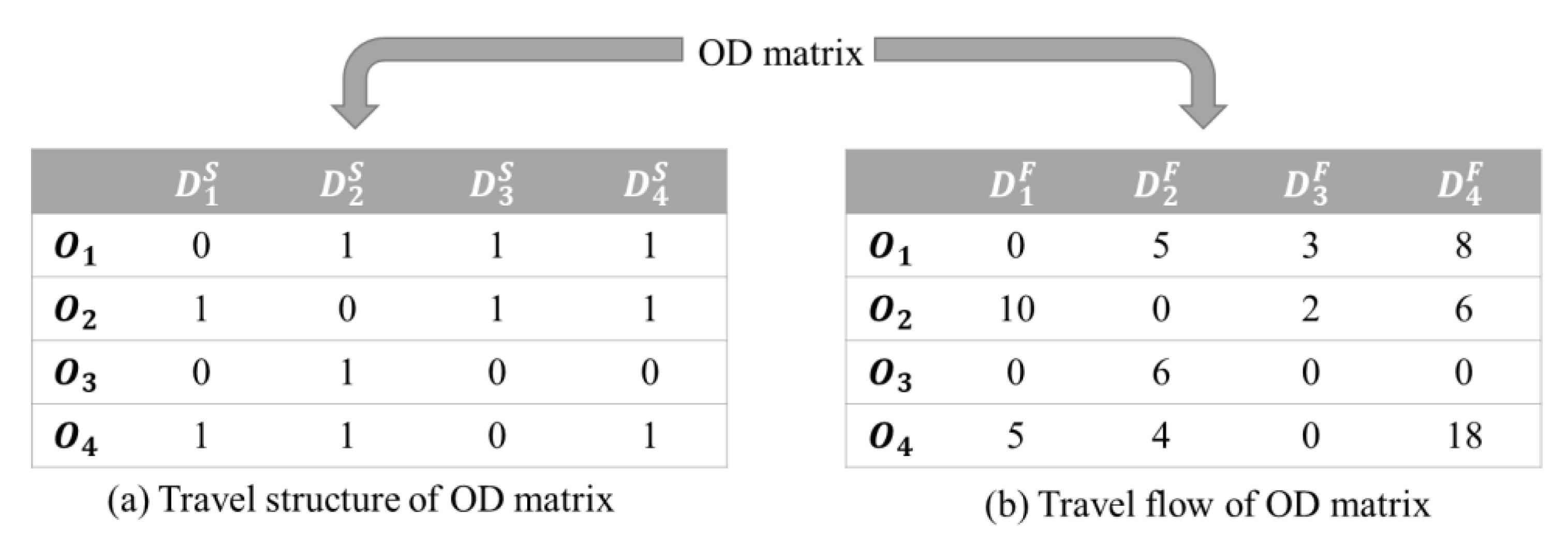
3.1. OD Matrix Construction

We use n predefined geographic units to group the OD of each journey. Each journey can be converted into a pair of ODs and described by ( O i ,   D j ) , where O i and D j indicate the geocodes of the corresponding units of the origin and destination points, respectively. Then, the OD matrix with n rows and n columns can be constructed by counting the number of journeys that started at O i and ended at D j . The OD matrix can contain information of the travel spatial structure and flow [1]. The travel spatial structure is the skeletal framework of the OD matrix, where the skeleton is expressed as the connectivity of the destinations from each origin. The travel flows corresponding to the structure are termed as a variable that describes the characteristics of the travel, such as volume and distance.
For instance, Figure 1a shows the spatial structure of the OD matrix. If there is a travel record between O i and Dj, we assigned the value of the spatial structure as 1; if not, then we assigned it as 0. Figure 1b shows the travel flow of the OD matrix, the value of each O i and D j assigned by their travel flow characteristic.

3.2. Stability Measurement of the Travel Spatial Structure and Flow

We use the similarity between the OD matrixes of different days to study the stability of interday taxi travel patterns. Specifically, the normalized Levenshtein distance for OD matrixes (NLOD) [1] based on Levenshtein distance expansion is adopted to quantify the difference between OD matrixes. To better understand the differences between the two OD matrixes, we developed two types of similarity measurements to reflect the spatial structure feature and the flow feature (the spatial structure and the volume of each OD pair).
(1)
Structural similarity
The travel structure indicates the spatial structure of the OD trips. As Equations (1) and (2) indicate, the calculation of the structural similarity S i m S T R between OD matrixes X and Y is transformed into the calculation of the edit distance S L D between the sets of the geocode of the destination location in different matrixes for the same original location code. g x i and g y i indicate the descending sorted geocodes of destination locations that started from the i-th geocode. To reduce the impacts of ODs with low traffic volume on structural similarity, the destination geocodes of the ODs with a flow number smaller than N 0 are removed in generating g x i and g y i .
S i m S T R ( x , y ) = 1 i = 0 i = n S N L D ( x i , y i ) n
S N L D ( x i , y i ) = S L D ( g x i , g y i ) l e n ( g x i ) + l e n ( g y i )
where S N L D is the normalized S L D ranging from 0 to 1, and l e n is an element counting function of a list. S L D calculates the Levenshtein distance between the geocode sequences constructed by the origin or destination locations based on the predefined geographical units. The Levenshtein distance measures the minimum number of single character edits, including insertions, deletions, and substitutions, required to change one string into the other. Specifically, approaches can be found in Navarro [34]. In this study, each character in the origin Levenshtein distance measurement is represented by the geocode.
Structural similarity can measure the similarity in the taxi travel spatial structure between different days. As mentioned above, a threshold number N0 is applied to reduce the impacts of the ODs with very low flow traffic volumes (e.g., only one trip for a specific pair of ODs). Evidently, the similarity level between different matrixes depends on N0. We test the sensitivity in the following sections.
(2)
Flow similarity
Compared with structural similarity, flow similarity S i m F L O W takes the number of trips for each OD into consideration when calculating the normalized similarity F N L D between the OD flow sequences f x i , f y i starting from the i-th geocode (Equations (3) and (4)). Note that the flow sequence consists of a list of geocode-volume pairs ( g i j , v i j ) , where g i j indicates the geocode j (ranging from 0 to m ) starting from geocode i , and v i j indicates the number of ( O i ,   D j ) trips. The number of trips v i j plays two roles in the calculation of F N L D : weighting the Levenshtein distance between f x i and f y i , obtaining the improved distance F L D ( f x i , f y i ) and normalizing the distance based on the sum of the number of trips in the OD flow sequence by the function f _ s u m to make F N L D range from 0 to 1.
S i m F L O W ( X , Y ) = 1 i = 0 i = n F N L D ( x i , y i ) n
F N L D ( x i , y i ) = F L D ( f x i , f y i ) f _ s u m ( f x i ) + f _ s u m ( f y i )
f _ s u m ( f i ) = j = 0 j = m v i j
The function F L D plays a key role in the calculation of flow similarity. The critical issue is how to weight the edit distance by volume. Specifically, for each pair of elements ( g x i j , v x i j ) and ( g y i j , v y i j ) in f x i and f y i , respectively, the weighted Levenshtein distance L ( j , j ) (Equation (6)) of this step could be calculated by the following rules: (1) if the geocode and the volume are the same, the most recent edit distance value does not change; (2) otherwise, the edit distance will be the minimum value from the following three situations: (a) L ( j 1 , j 1 ) + a b s ( v x i j , v y i j )   i f   g x i j = g y i j , which means that the geocode is the same and only the traffic volume needs to be changed; (b) L ( j 1 , j ) + v x i j   i f   g x i j g x i j which means that the element ( g i j , v i j ) in f x i needs to be added, and (c) L ( j , j 1 ) + v y i j   i f   g x i j g x i j , which means that the element ( g y i j , v y i j ) in f y i needs to be deleted. For more specifics on this approach, refer to NLOD (Behara et al., 2020) [4].
L ( j , j ) = { L ( j 1 , j 1 )         g x i j = g y i j   a n d   v x i j = v y i j min ( L ( j 1 , j 1 ) + a b s ( v x i j , v y i j ) L ( j 1 , j ) + v x i j L ( j , j 1 ) + v y i j ) o t h e r w i s e

3.3. Stability Measurement of Each OD Flow

We adopted the coefficient of variation method to measure the interday stability in the volume of trips between different regions. The coefficient of variation VAR is the ratio of the standard deviation F V S D to the average F V M (Equations (7)–(9)). V A R can be adjusted to measure the stability of the number for the same OD pairs on different days.
V A R i j = F V S D i j F V M i j
F V M i j = w = 1 w = W F V i j w W
F V S D i j = w = 1 W ( F V i j w F V M i j ) 2 W
where F V i j w is the flow volume on day w between geographic units i and j , and W is the days of the dataset.
To better classify the type of OD pairs, we divide F V M i j and stability according to the combination of flow volume and variability quartiles, respectively (Figure 2). The specific rules are shown in Equations (10) and (11), where Q1 and Q3 are functions for calculating the first and third quantiles. For example, HL in Figure 2 represents ODs with a relatively high flow volume and low stability, which means that the travel demand of this pair of ODs is large but varies greatly across days.
F V L e v e l = { H ,                               F V M i j > Q 3 ( F V M i j ) M ,       Q 3 ( F V M i j ) F V M i j Q 3 ( F V M i j ) L ,                               F V M i j < Q 1 ( F V M i j )
S T A L e v e l = { L ,                               V A R i j > Q 3 ( V A R i j ) M ,       Q 1 ( V A R i j ) V A R i j Q 3 ( V A R i j ) H ,                               V A R i j < Q 1 ( V A R i j )

4. Data

Two datasets are adopted to analyze the taxi travel characteristics between days. Our study area includes Shen Zhen in China and New York in the United States. They are both the city with thriving economies and trade [35]. Note that the first dataset (DT1) consists of the raw taxi trajectory records, while the second dataset (DT2) consists of the OD trip records directly. Different datasets correspond to different data process flows.

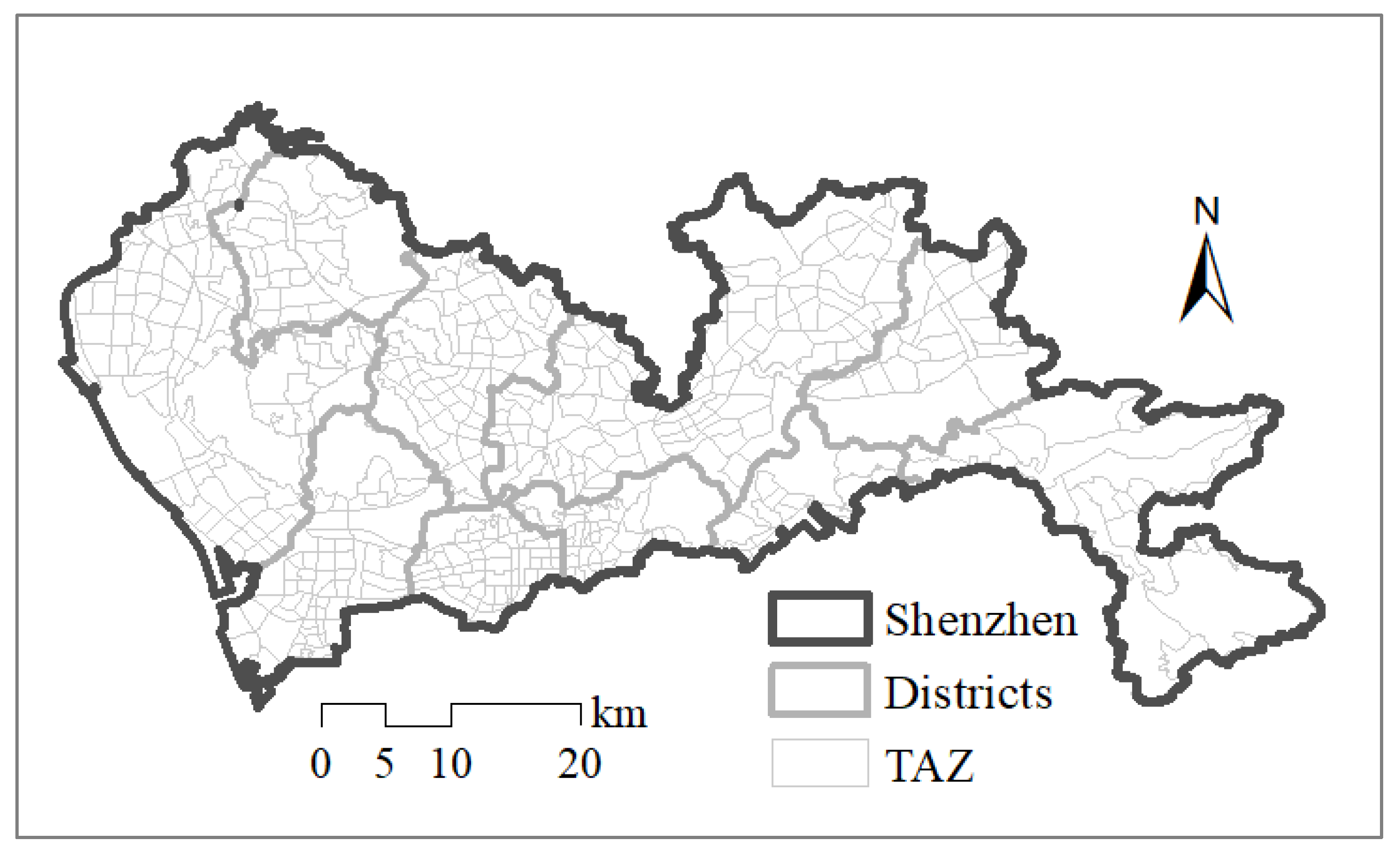
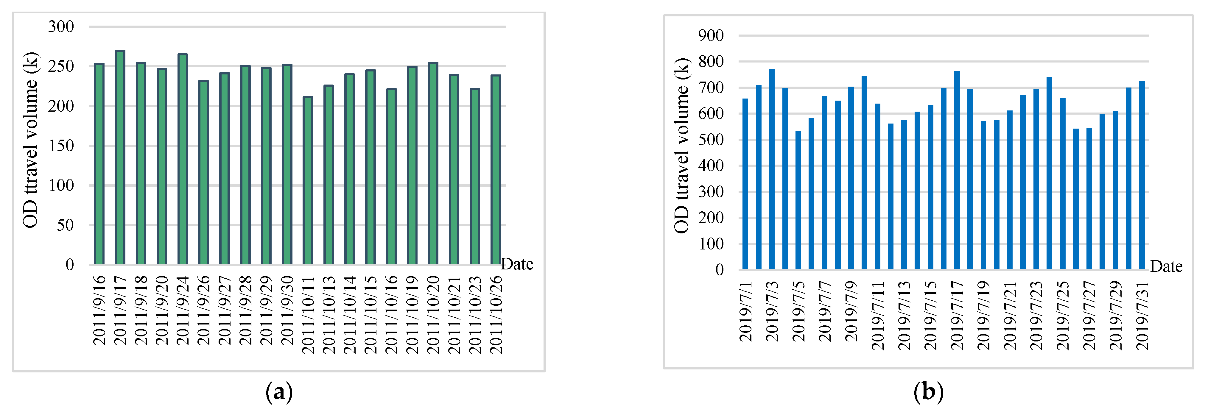
4.1. Dataset of Shenzhen

The first dataset (DT1) corresponds to Shenzhen, which is located in southern China, southern Guangdong, and adjacent to Hong Kong. Since its establishment in 1979 as a Special Economic Zone (SEZ) of China, Shenzhen has become one of the largest and most innovative cities in China [36] and is one of the fastest-growing and densely populated metropolitan cities in the world. It is located south of the Tropic of Cancer. Shenzhen has 9 districts, with a total area of 1997.47 square kilometers. Shenzhen has complete transportation facilities, such as subways, buses, and taxis, so it is convenient for residents to travel, which makes Shenzhen a good case area for travel pattern research [37].
The raw taxi trajectory data include the operating trajectory data of approximately 17,000 taxis from 16 September to 28 October 2011. The data include device number, longitude, latitude, positioning time, and passenger load status (passenger load is 1, the empty load is 0), as shown in Table 1. We use the TAZs as geographic units to analyze the passenger travel OD. Shenzhen can be divided into 491 TAZs, with an average area of 3.98 km 2 (Figure 3).
We first conduct an exploratory data analysis on the number of records of the raw data and the number of vehicles and exclude data with obvious abnormalities (such as missing data in a certain period) of DT1. To reduce the impact of changes in the number of vehicles, we select the Shenzhen trajectory data of 7289 vehicles that have data every day. As a result, 20 days of data are kept, covering all weekdays and weekends, and each date type (i.e., weekend and weekday) includes at least two days of data (see the Supplement for specific analysis).
Then, the OD trips for each vehicle are extracted according to the switch patterns of passenger load status. The number of ODs per day is approximately 428,600.

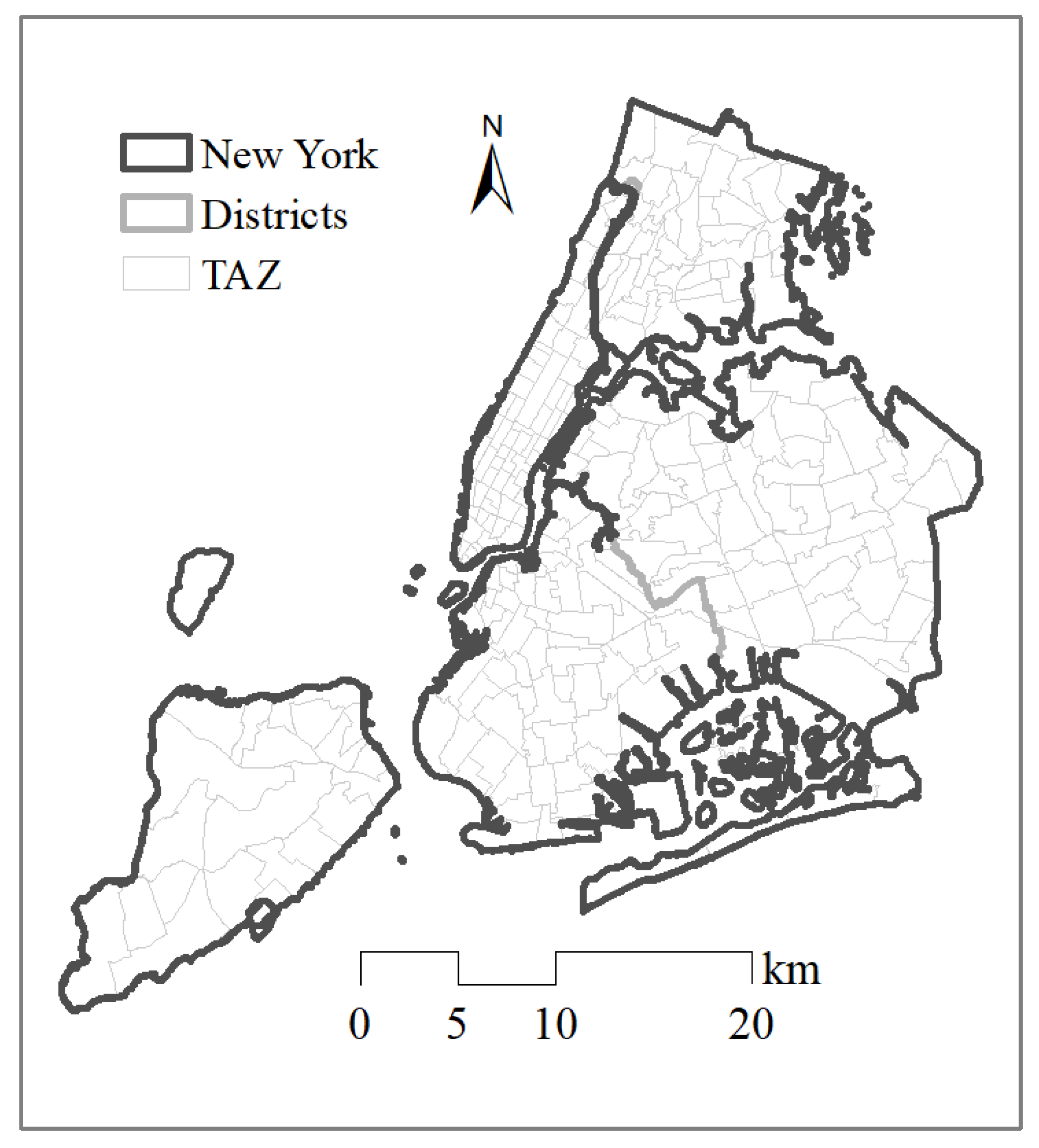
4.2. Dataset of New York

The second dataset (DT2) corresponds to New York City (NYC), a worldwide famous international city in the USA. New York City is one of the largest cities and the most densely populated major city in the world. It has 302.6 square miles and five boroughs, including Brooklyn, Queens, Manhattan, Staten Island, and Bronx. New York City is a global cultural, financial, and media center with a significant influence on commerce, health care, and life sciences [38]. New York has a good transit service [26], and its taxi rides form the core of the traffic in the city [39].
In recent years, the promotion of the open data policy in New York City has provided great convenience and opportunities for big data researchers [40]. The datasets are collected by the NYC Taxi and Limousine Commission and can be downloaded from the official website (https://www1.nyc.gov/site/tlc/about/tlc-trip-record-data.page, accessed on 1 December 2020). We select the High Volume For-Hire Vehicle trips records during 1 and 31 August 2019, as DT2 to analyze the taxi travel spatial structure in NYC. Each row DT2 represents a trip record, including pickup date-time, drop-off date-time, pickup location ID, and drop-off location ID (Table 2). In addition, we regard the taxi zones the NYC Taxi Administration provided as TAZs. There are 264 TAZs in the study, and Newark outside NYC is included in the following analysis (Figure 4). Since the records of DT2 are the OD trips directly, we did not further process the data.

5. Results

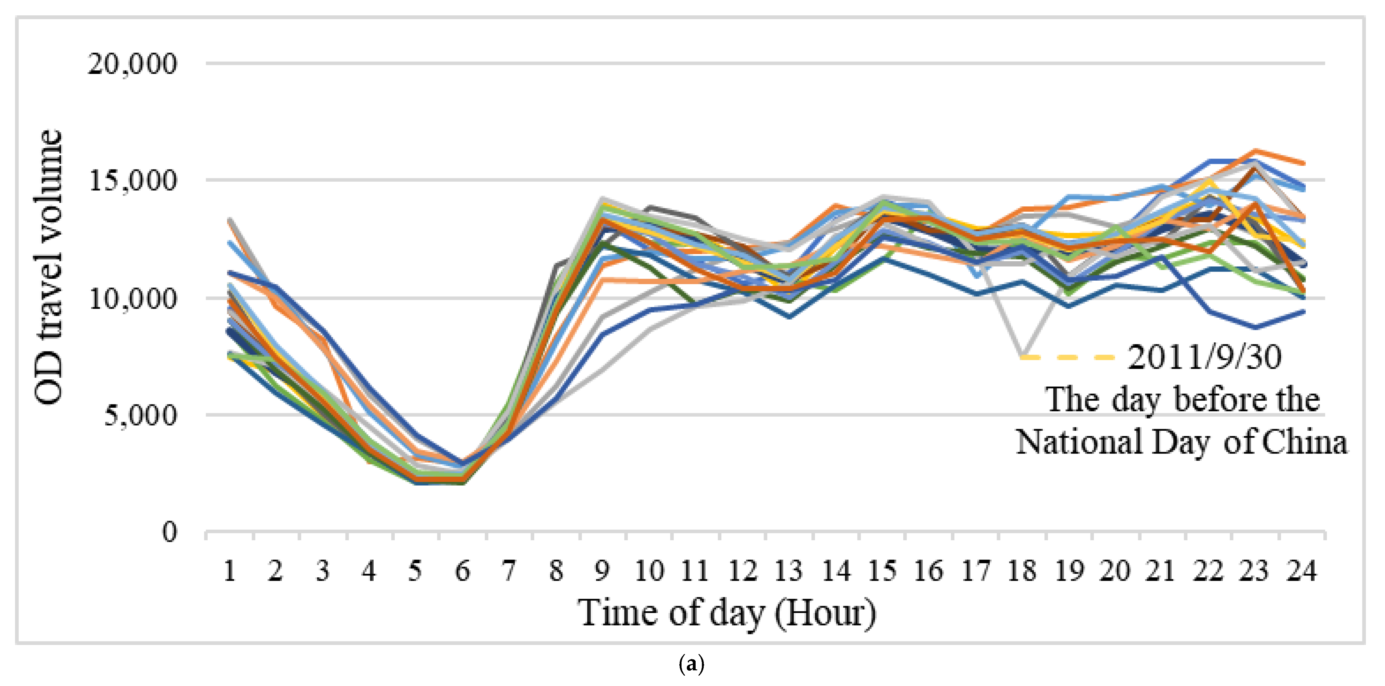
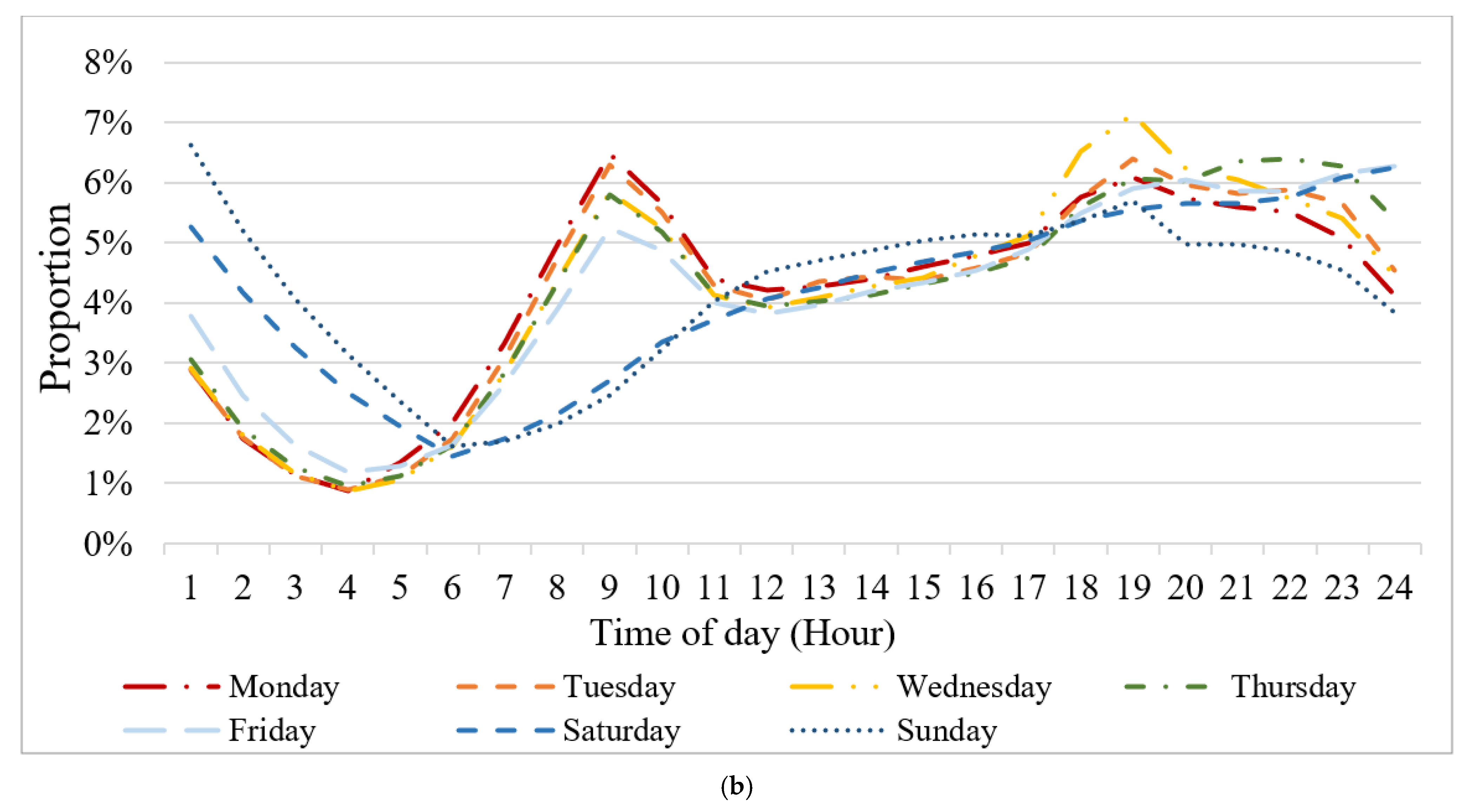
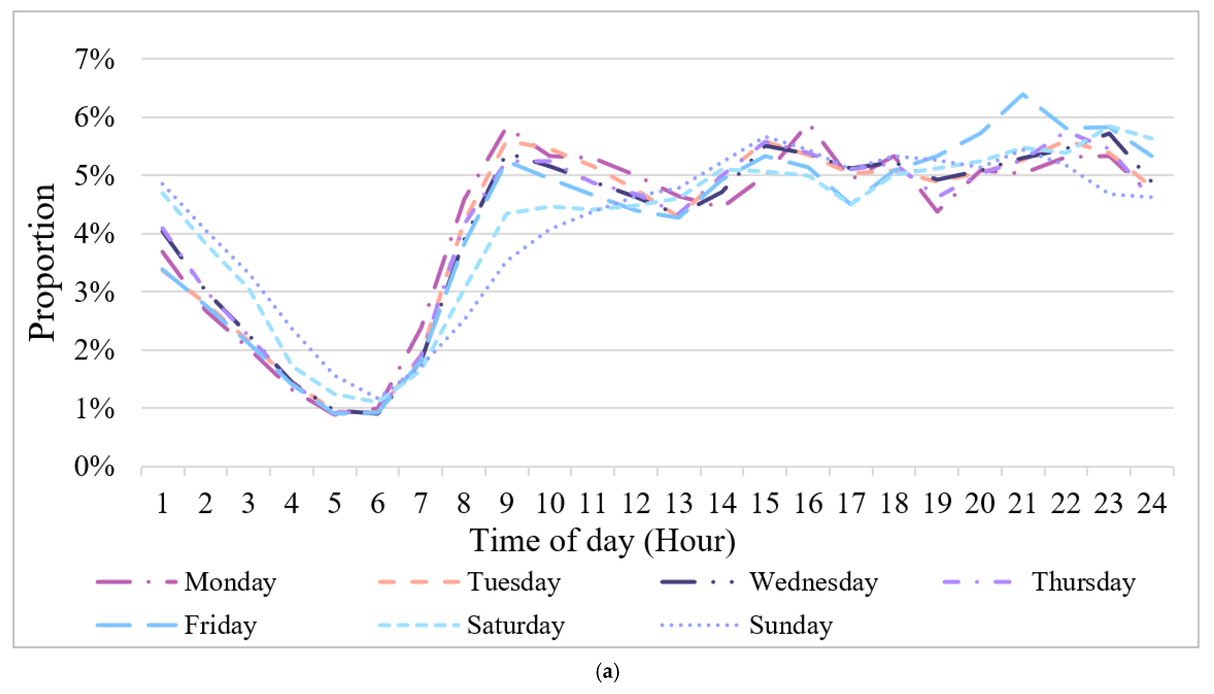
5.1. Volume and Distance Characteristics of Interday Taxi Travel

Figure 5 shows the daily OD travel volume and distance in weeks. The daily trip frequency falls between 200,000 and 270,000 in Shenzhen, with the average daily OD for each taxi ranging from 27 to 37. The daily trip frequency of NYC falls between 530,000 and 780,000, which is higher than twice that of Shenzhen.
Figure 6 shows the hourly characteristics of the OD flow. The 20-day data of Shenzhen exhibit a relatively similar general hourly distribution pattern (Figure 6a): the travel activities gradually decrease from 0 to 6 in the early morning and increase rapidly from 6 to 9 during the morning peak hours. No obvious night peak pattern is observed. There is no clear difference between weekdays and weekends. Only one sudden drop in OD trips is observed at approximately 18:00 on 30 September, which is mainly caused by the night peak congestion before the 7-day holiday of National Day of China. Compared with Shenzhen, the hourly distribution of NYC exhibits two different types of hourly patterns (Figure 6b), which correspond to the weekday pattern and weekend pattern, respectively (Figure 7b).
Figure 7 shows the hourly distribution characteristics of the OD travel volume from Monday to Sunday. The hourly travel volume on weekdays and weekends exhibits some different patterns in both Shenzhen and NYC. The number of trips on weekend nights is higher than that on weekdays. An obvious morning peak can be observed at 9:00 on weekdays, which is mainly driven by morning commuting trips. This pattern is not observed on weekends. The early mornings during 0:00–6:00 on Saturday and Sunday exhibit a higher travel demand than those on weekdays, which is mainly caused by trips related to the increase in entertainment activities during the weekends.
Friday nights (20:00–24:00) exhibit more travel demand than other weekday night periods and are similar to Saturday nights. In addition, the travel demand on Sunday exhibits a significant decrease after 21:00, but Sunday’s volume decreases the least. The potential reason is that people tend to arrange more activities on Friday nights since this night directly leads into the weekend, while Sunday nights precede a work day, and people prefer to rest to prepare themselves at home. These two results imply that Friday nights and Sunday nights have different patterns than other weekdays and weekend days, respectively. Separate policies may be needed for these two periods to avoid potential misleading decision making related to transportation services.

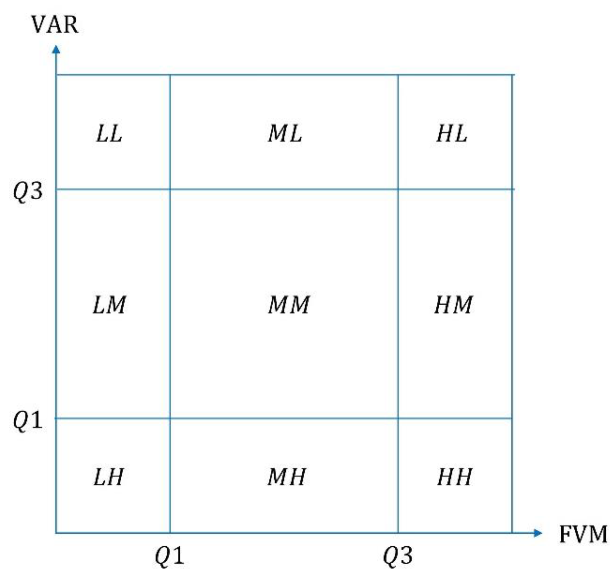
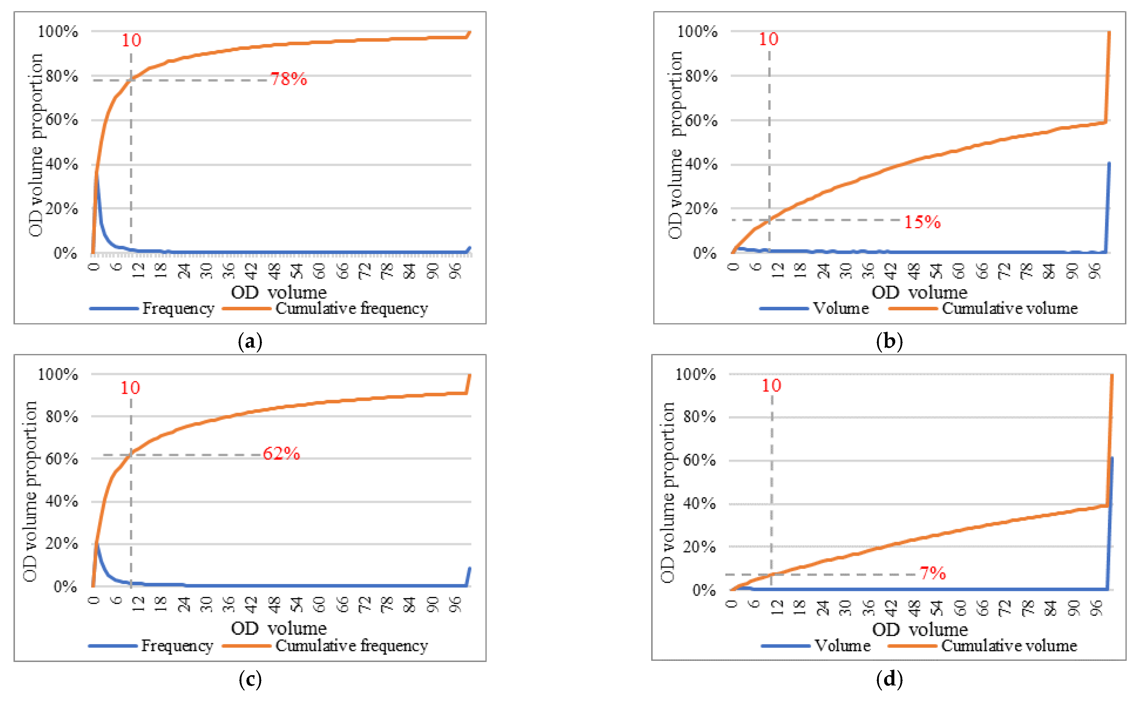
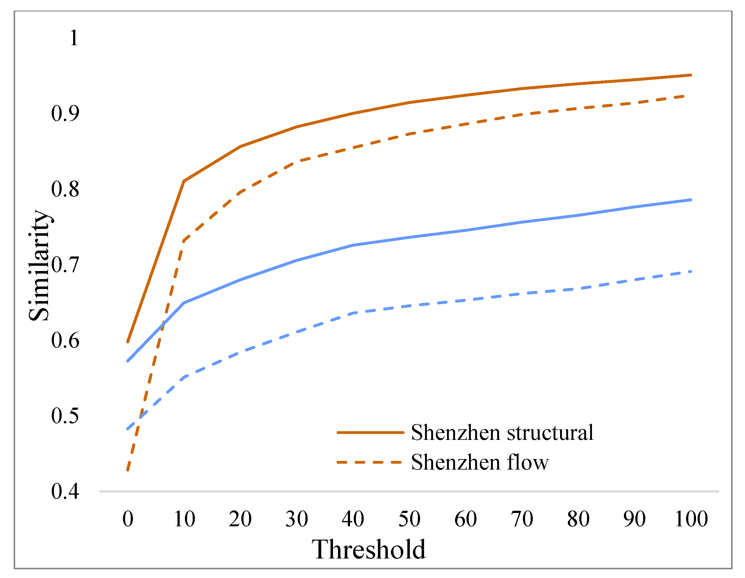
5.2. Influence of the Flow Threshold on the Similarity in the Travel OD Flow Matrix

In Figure 8, taxi travel OD shows a heavy-tailed distribution, which means that a large number of ODs have a small volume. The number of ODs gradually decreases with increasing OD volume, as shown in Figure 7a,c. For example, there are 12,905 ODs between TAZs with fewer than 10 flows in Shenzhen, accounting for 78% of all TAZ ODs, but their cumulative volume only accounts for 15% of all flows, as shown in Figure 7b. In NYC, there are 11,296 ODs between zones with fewer than 10 flows in Shenzhen, accounting for 62% of all zone ODs, but their cumulative volume only accounts for 7% of all flows, as shown in Figure 7d. These ODs make limited contributions to the whole picture of the travel flows but will lead to obvious impacts on the description of travel patterns. Usually, a traffic volume threshold is applied in existing studies [41] to remove these ODs and reduce their negative impacts.
When calculating the similarity of the OD matrix in this paper, we found that different thresholds have impacts on the similarity result. To reasonably select the threshold, we tested the similarity changes in the OD matrix based on the travel spatial structure and travel flow under different thresholds (Figure 9). The similarity increases with the threshold. When the threshold is greater than 10, the similarity growth rate slows down and tends to be stable in Shenzhen. In this study, we selected ODs with a flow volume greater than 10 to analyze the structural and flow similarities, and NYC’s threshold remains the same as Shenzhen’s.

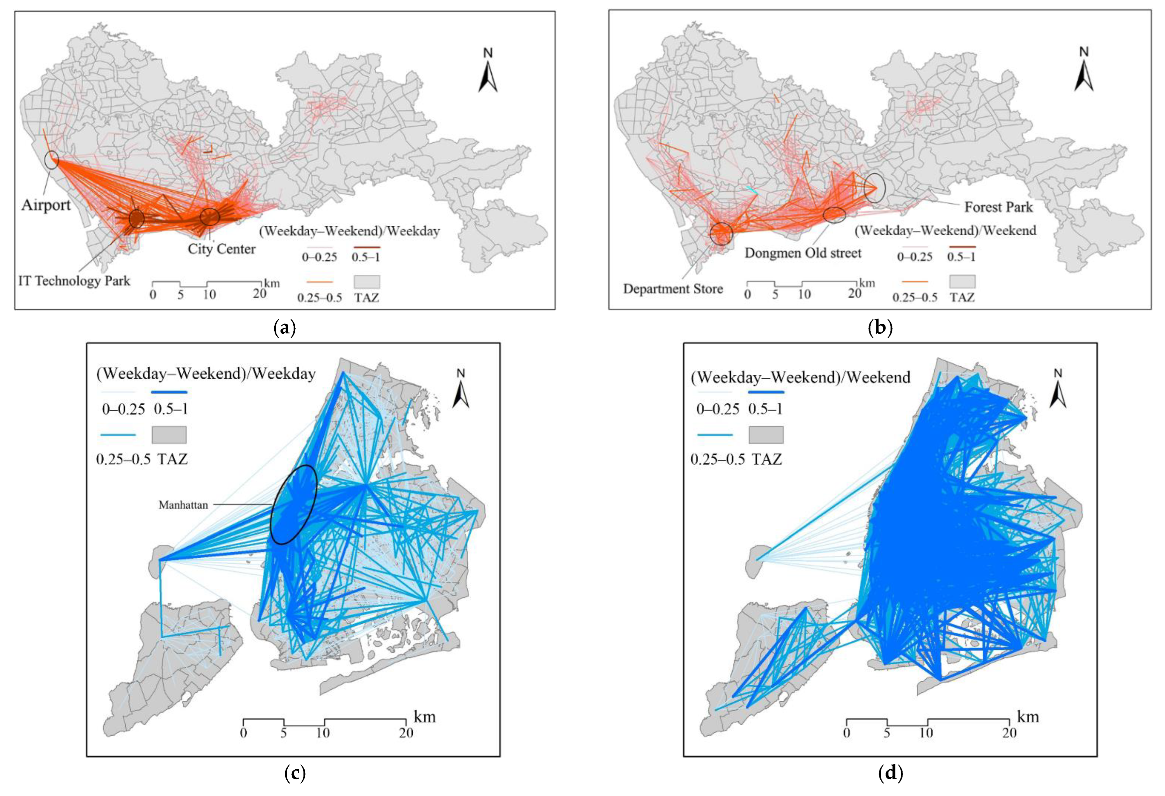
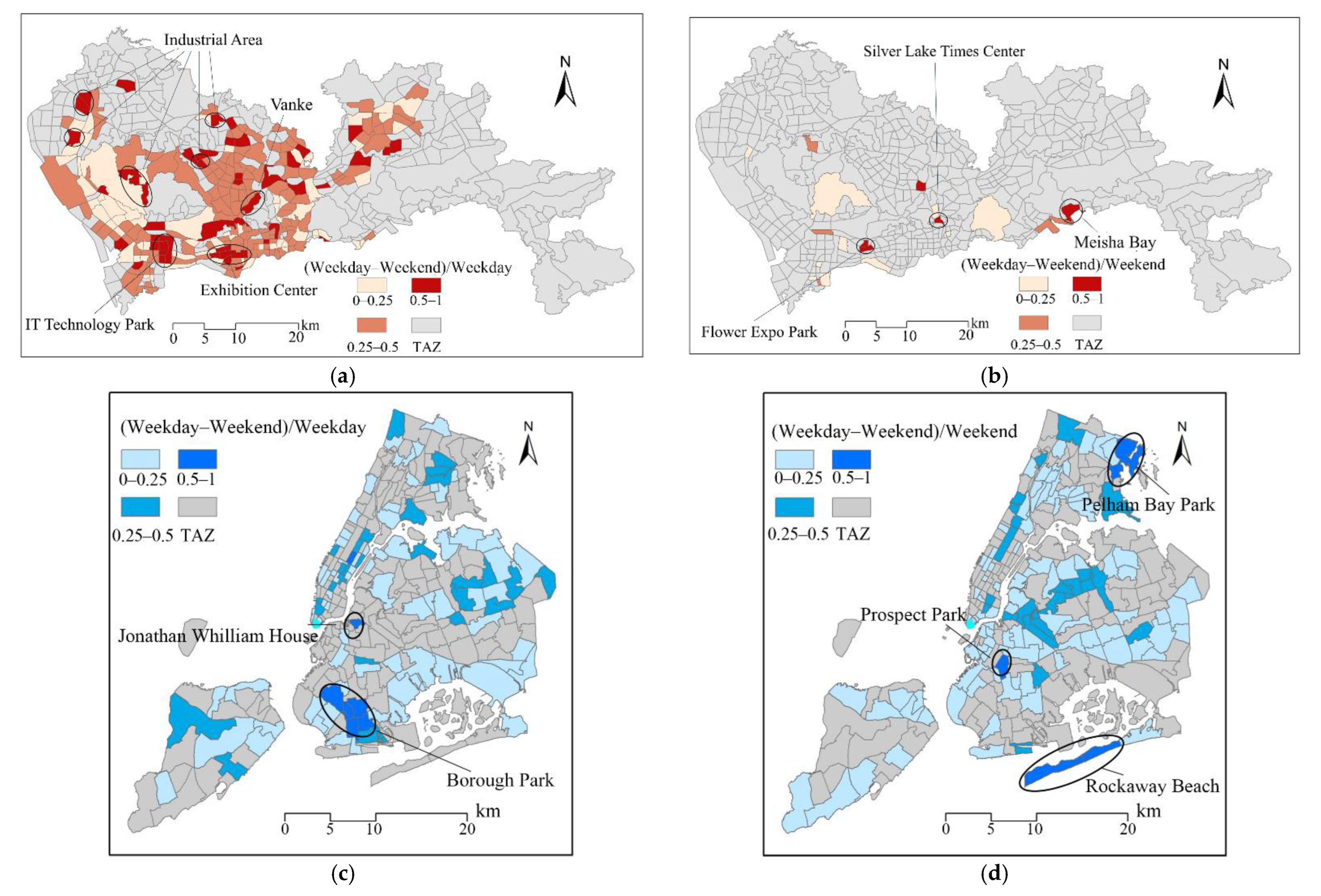
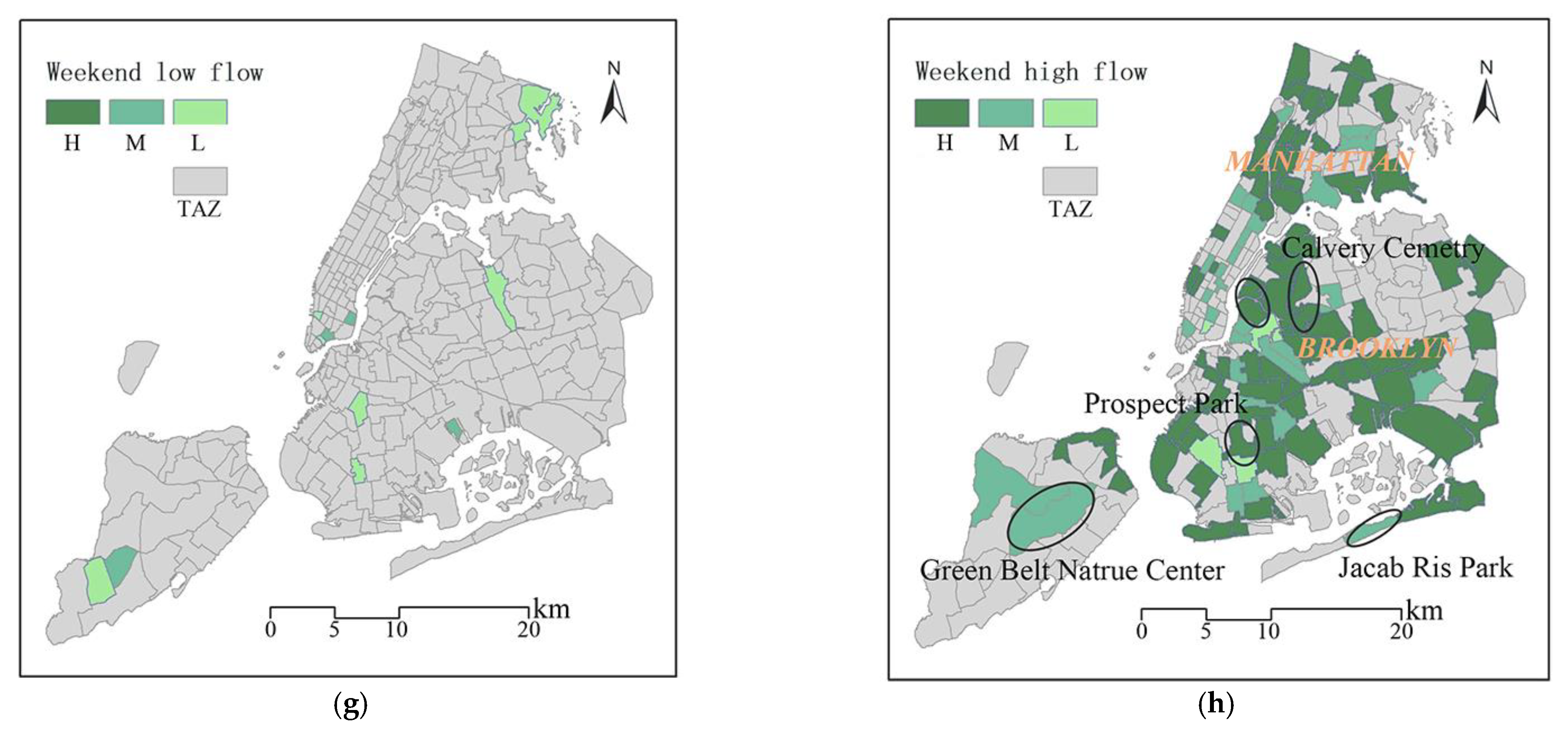
5.3. Stability of Travel Spatial Structure and Flow between Weekdays and Weekends

Table 3 and Table 4 show the 20-day taxi travel spatial structure similarity and flow similarity organized by the day of the week in Shenzhen, and Table 5 and Table 6 show the 31-day taxi travel spatial structure similarity and flow similarity in NYC. We find that the dark blue background color (low similarity) is mainly distributed in the upper right corner and the lower left corner. This indicates that the similarity between weekdays and weekends is significantly lower than that between weekdays and between weekends days. In the results corresponding to Saturday and Sunday, the background color of Friday is lighter than other days, which means that the similarity between Friday and the weekends is higher than the similarity between other working days and the weekends. This finding coincides with the special pattern presented in Section 5.1. In addition, the structural similarity between the days is higher than the flow similarity, which also shows that a similarity measure considering the flow can reflect the detailed differences between the row OD matrix.
To better understand the travel patterns on different days, we visualize the spatial distribution of ODs for taxi travel between geographic units and within each geographic unit on weekdays and weekends (Figure 10 and Figure 11; the detailed distribution during daily and weekday, weekend OD can be found in the Appendix A and Appendix B).
From the perspective of internal travel within a geographic unit, for ODs with more than 10 trips, 92.83% of TAZs have an internal travel volume on weekdays greater than that on weekends in Shenzhen. These are mainly workplaces, including IT Technology Park, industrial zones, Vanke, the Convention and Exhibition Center, and other areas (Figure 10c). There are only 20 TAZs where the number of trips within the TAZ on weekends is greater than that on weekdays. These are mainly entertainment areas such as Shenzhen Bay, Meisha Bay, Flower Expo Park, and Silver Lake Times Center (Figure 10d). However, 51% of TAZs have an internal travel volume on weekends greater than that on weekdays in NYC. Areas with large differences are mainly parks and residential areas, including Rockaway Park, Pelham Bay Park, and other areas.
From the perspective of travel between geographic units for ODs with more than 10 trips, 65% of the travel flow between TAZs on weekdays is greater than that on weekends in Shenzhen. These TAZs are mainly concentrated in two places: IT Technology Park and its surrounding areas, the City Center and its surrounding areas, such as Huaqiang North Commercial Area, the Science Museum, and other areas. Another obvious feature is that the travel flow between the airport and these areas is also significantly increased (Figure 11c). These regions are mainly related to workplaces and business concerns. In contrast, the travel flow distribution that emerges on weekends is scattered and related to entertainment areas such as the Haiya Department Store, China Resources Vanguard, Forest Park, and Futian Station (Figure 11d). However, 27% of the travel flow between geographic units on weekdays is greater than that on weekends in NYC. These zones are mainly concentrated in Manhattan areas and interact between Manhattan and other areas. On weekends, cross-regional taxi travel activities increased significantly compared to weekdays.

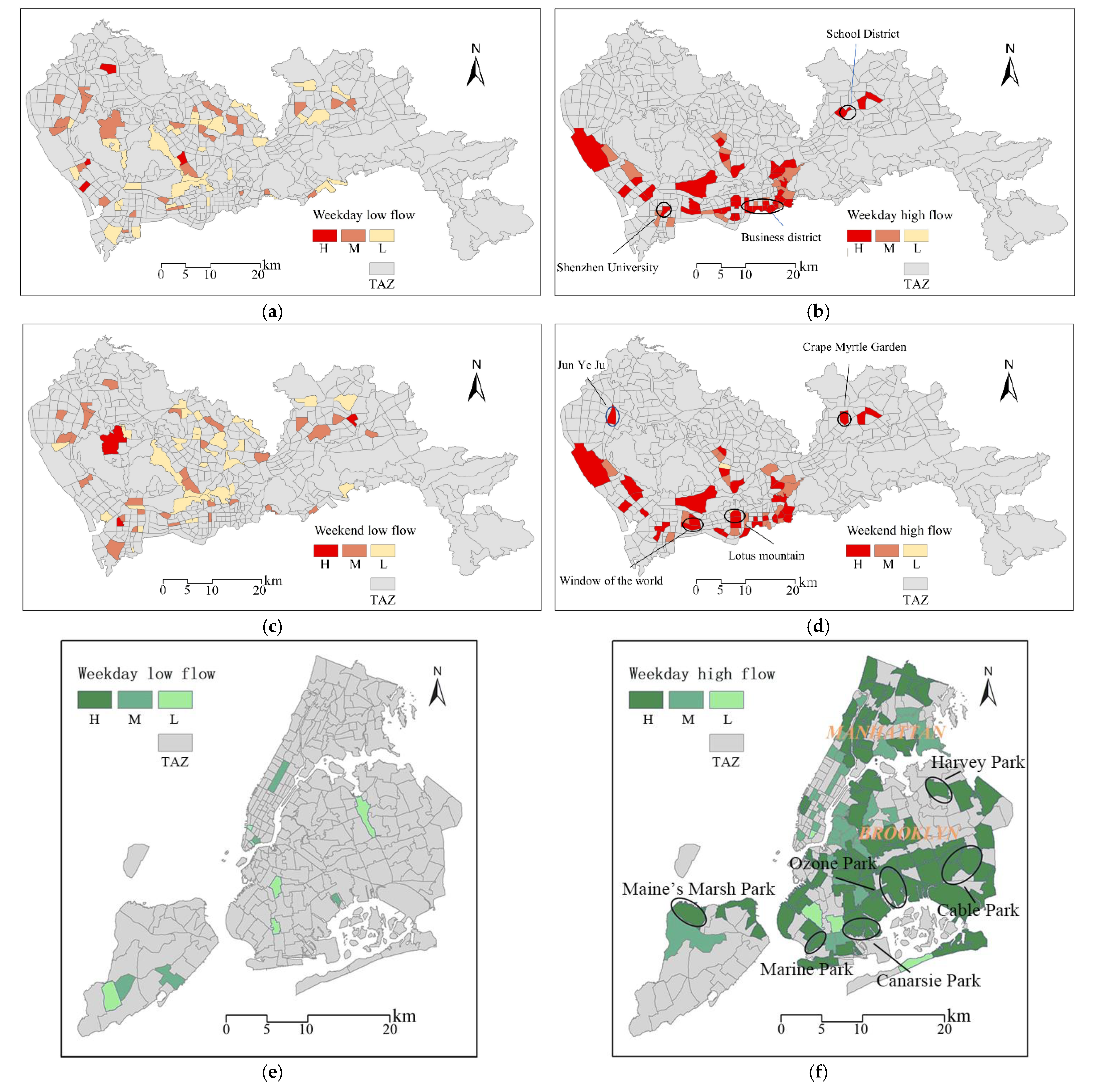
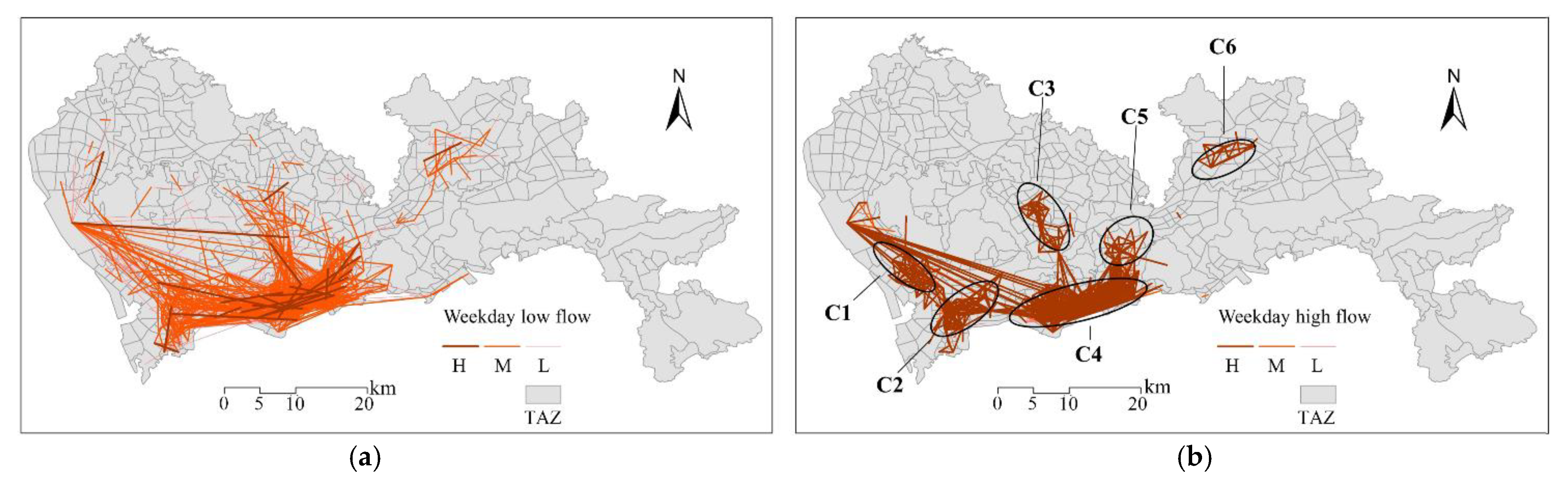
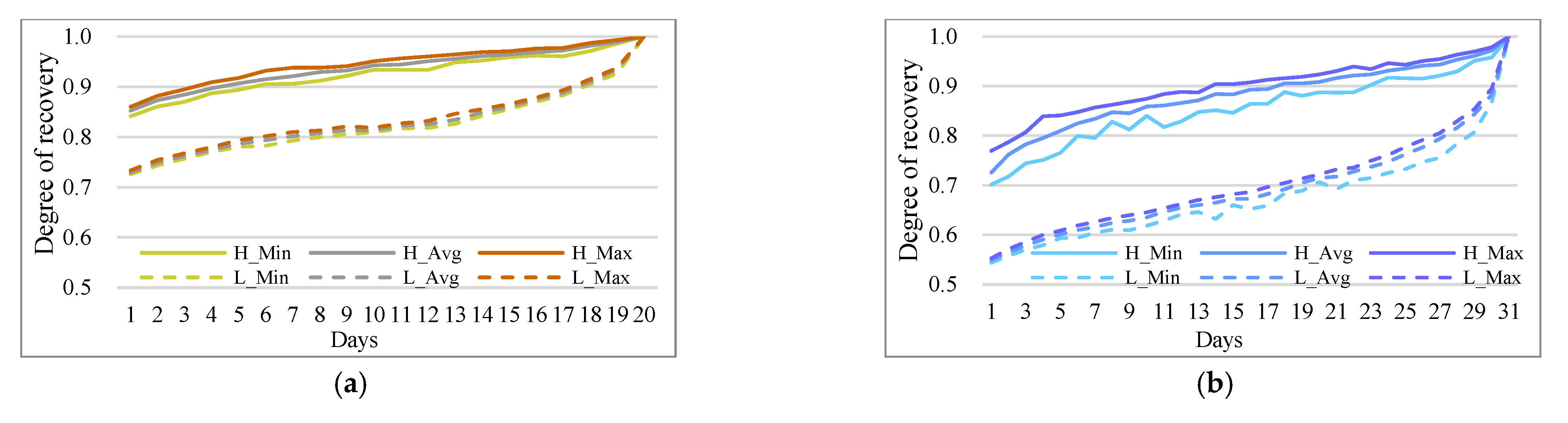
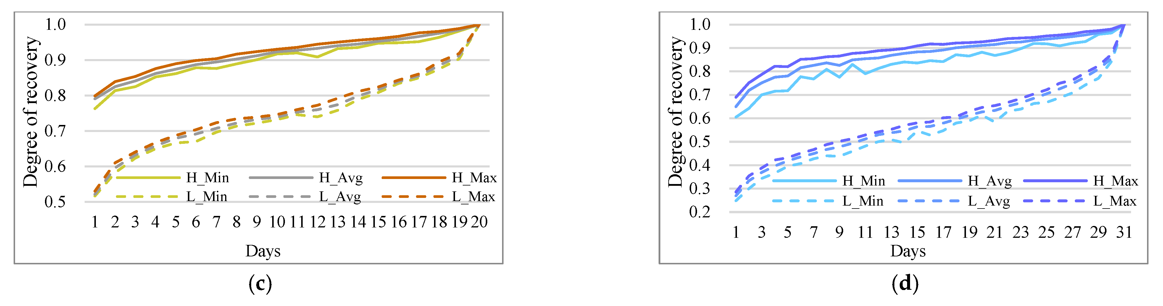
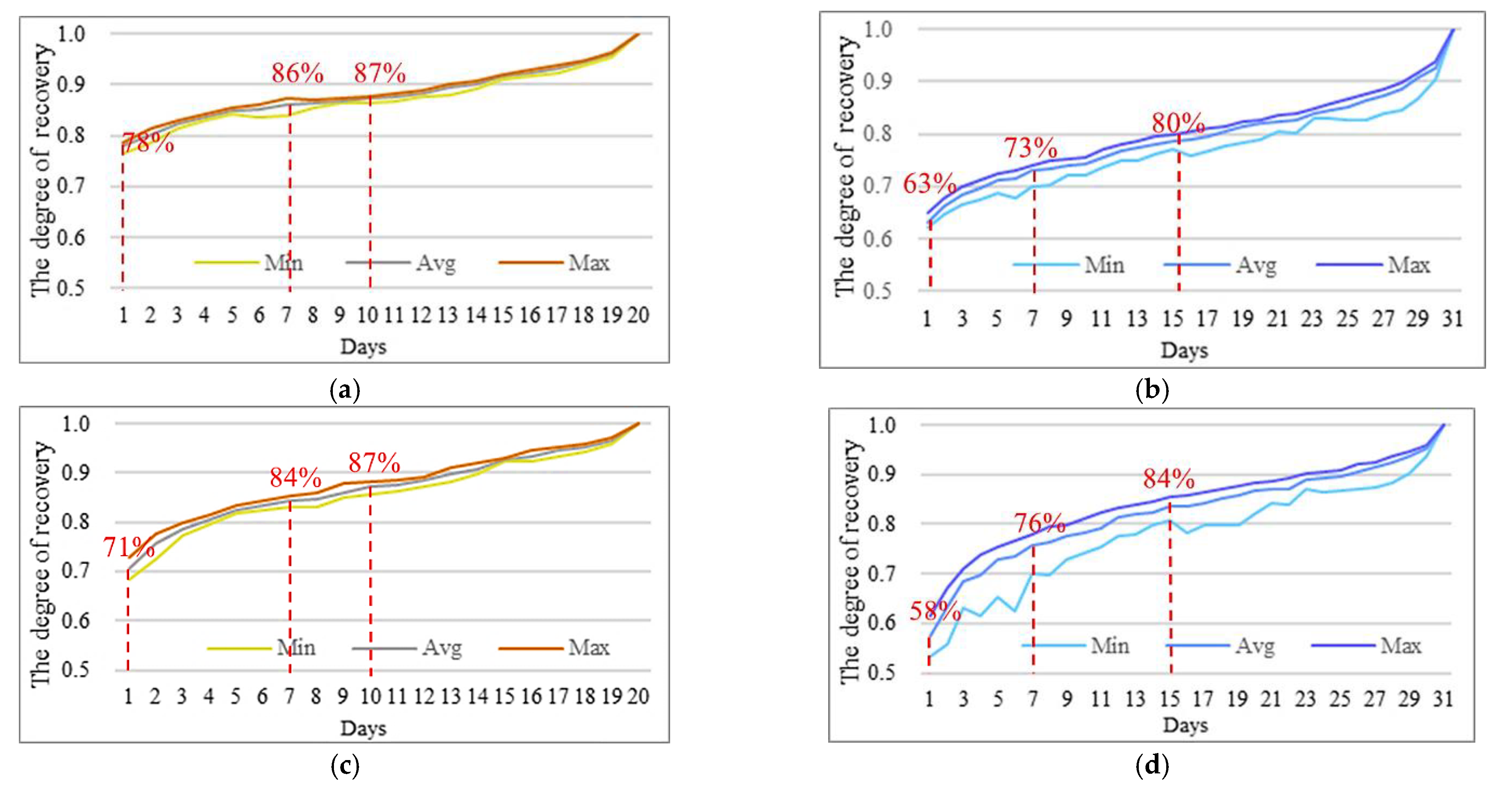
5.4. Stability of OD Flows between Days

Based on the OD flow stability measurement method, we separately analyzed the changes in the stability of the geographic unit and between regions during weekday and weekend stability. (Figure 12 and Figure 13). Figure 12 shows the change in internal geographic unit travel stability based on traffic flow during weekdays and weekends. The overall high-traffic and high-stability areas are located in the Baoan Airport area, Futian Port, Huaqiang South, Technology Industrial Park, and other areas in Shenzhen. Office buildings and schools in the TAZs (e.g., Huaqiangbei, Dongmen, Old Street Commercial District, and Shenzhen University Area) on weekdays have a relatively stable and large traffic volume and a smaller volume during the weekend. In addition, TAZs with more diversified internal functions (such as Crape Myrtle Garden and the area near Junyeju) will have relatively higher stability on weekends (Figure 12f). Short-distance travel contributed to a stable traffic flow. In New York, Brooklyn and Manhattan are more stable on weekdays than the internal travel flow on weekends. Correspondingly, areas with more stable weekend trips generally have parks, and the regional infrastructure functions are relatively complete.
The stability and distribution of travel flows between geographic units are shown in Figure 13. In the spatial distribution, high-stability, high-flow TAZ interactions mainly occur in six areas in Shenzhen, especially on working days: Baoan District Golden Terrace Industrial Zone (C1), IT Technology Park (C2), Longua Metro Station neighborhood (C3), Huaqiang North Business District, Fukuda Port, Dongmen Old Street Business District and other more interactive areas (C4), Shenzhen East Station and its surrounding areas (C5), Longgang District Longcheng Park and Crape Myrtle Garden (C6). These areas are more stable between weekdays and weekends. In the low-traffic travel ODs, the spatial distribution of stable and high-level ODs varies widely, fully reflecting differences in travel patterns on weekdays and weekends. In New York, we found that the interactive traffic between the three airports and Manhattan, Brooklyn, and Queens is large and stable. In response to this phenomenon, we can increase public transportation configuration and reduce ground traffic congestion. Compared with weekdays, stable taxis travel farther between areas on weekends.
These findings can be used to guide real-life urban transportation planning. In regions with high traffic volumes and high stability in taxi trips, public transportation services (e.g., regional buses) could be added to reduce taxi usage and increase the share of public transit. This will improve transportation efficiency and reduce related air pollutants and carbon emissions. For regions with high traffic volume but low stability in taxi trips, understanding temporal patterns could help to optimize the dispatching of taxis and online car-hailing services. For example, more online car hailing could be encouraged and guided to fulfill travel demand during the morning peak hours near the “hotlines”. In addition, if there is a significant difference between weekdays and weekends, the relevant departments should increase the supply of public transportation services at the corresponding time to promote public travel by public transportation.
For travel characterized by the low flow between regions, we need to combine other data to analyze the reasons for the low travel flow and then explore possible solutions.

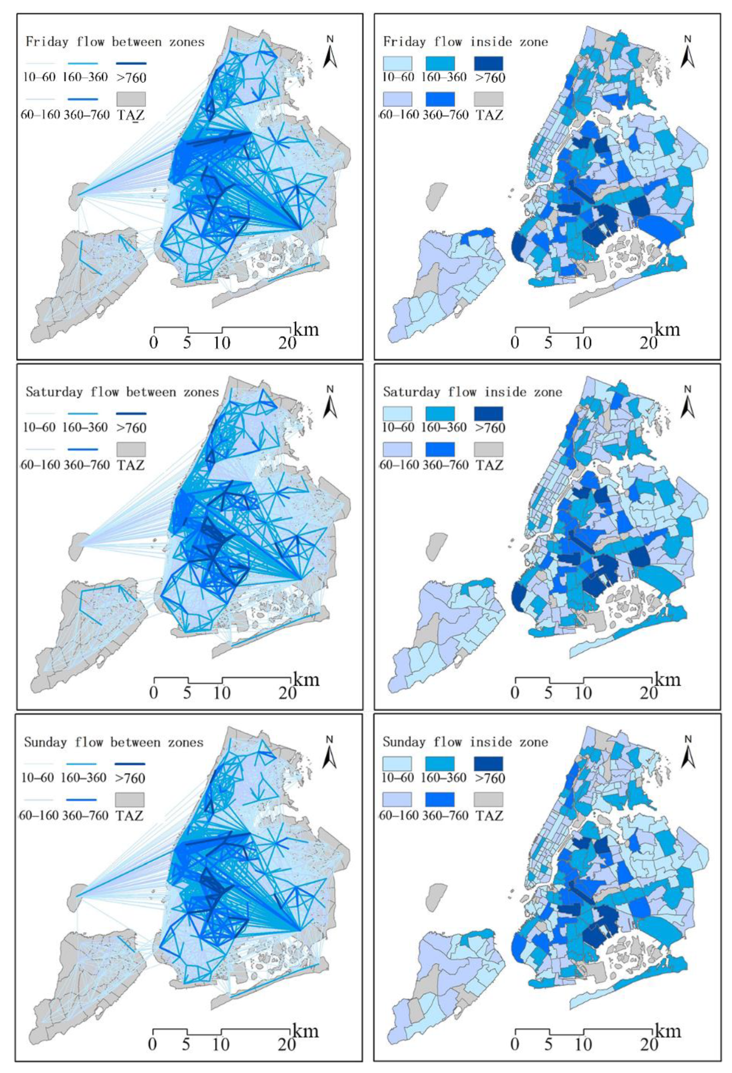
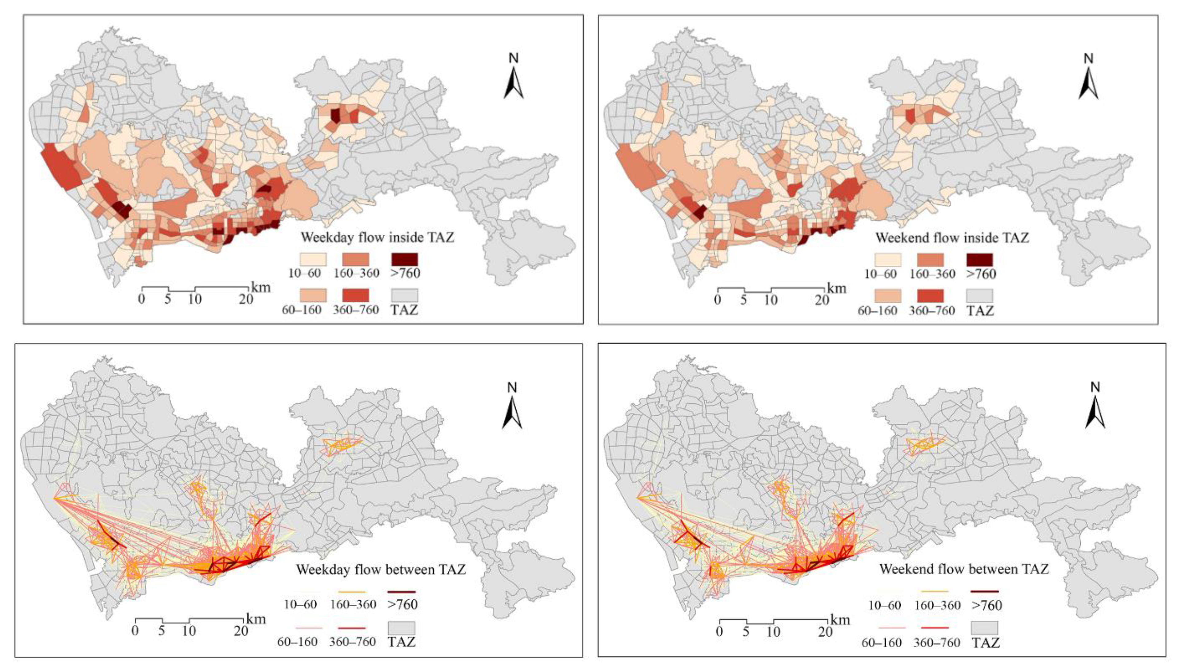
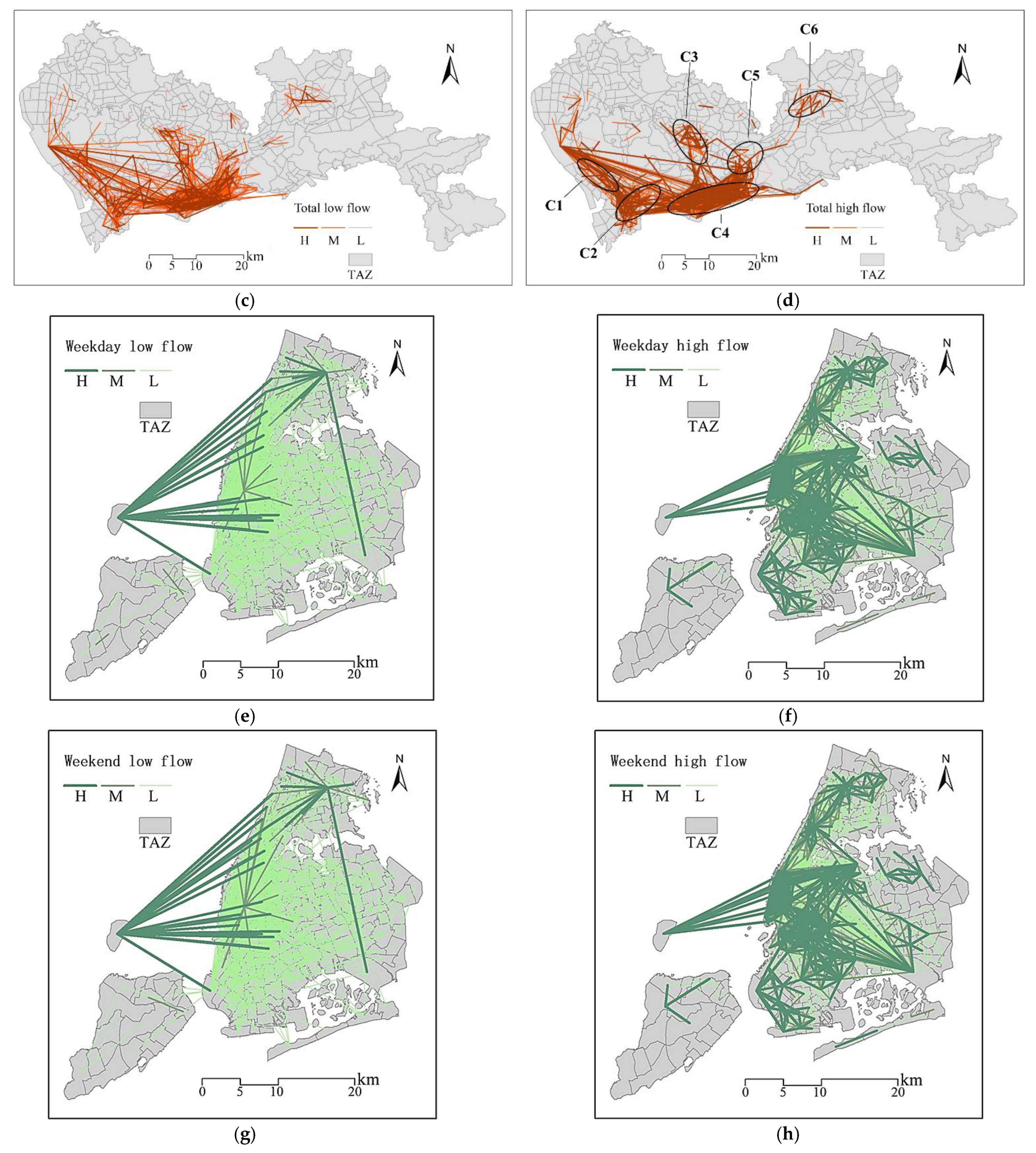
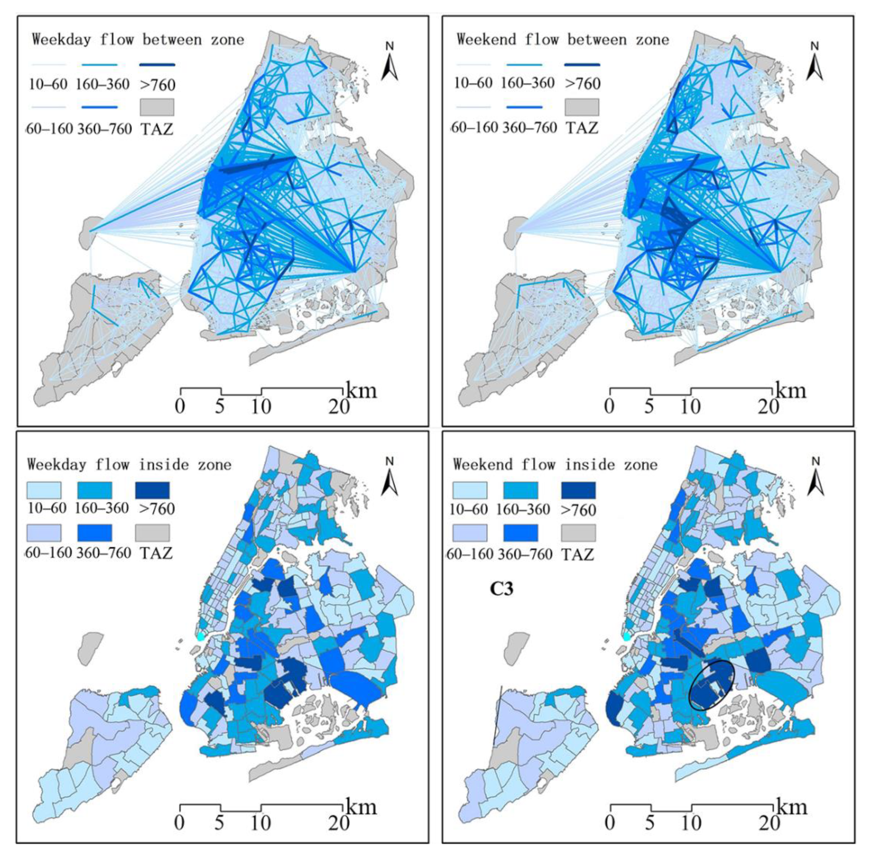
5.5. Representative Data Analysis

The previous analysis shows certain similarities and obvious differences in the interday taxi travel structure, which means that the results from an analysis of taxi travel spatial structure have a certain dependence on the choice of data. Therefore, we further compared the difference between the taxi travel OD obtained from the coverage data for different days and that for the whole dataset to analyze the impact of data selection on the results. To this end, we randomly select data from different days and calculate the average daily matrix of OD between different TAZs.
The structural similarity and flow similarity between the OD matrix derived from different days and the OD matrix derived from the whole dataset are calculated and compared. A high similarity level indicates that the selected day data can represent the overall data well. To reduce the influence of chance selection given the number of days, we randomly select 10 sets of days for each set size from the whole dataset. The maximum, minimum, and average values of the similarity are calculated. We conducted experiments based on two datasets, Shenzhen and New York City. Figure 13 and Figure 14 indicate that one day’s data can describe 78% of the overall travel spatial structure and 71% of the travel flow in Shenzhen, while a week of data can describe 86% of the overall travel spatial structure and 84% of the travel flow. In addition, one day’s data can describe 63% of the overall travel spatial structure and 58% of the travel flow in NYC, while a week of data can describe 73% of the overall travel spatial structure and 76% of the travel flow. Half of the data in the two datasets can describe 87% of the overall travel spatial structure and 87% of the travel flow in Shenzhen, and it can describe 80% of the overall travel spatial structure and 84% of the travel flow in NYC.
On the one hand, this result can be used to evaluate the reliability of the analysis results obtained based on the taxi data; for example, one day’s data, randomly selected, can reflect 50% of the overall data, at least in different cities. In addition, the results can also be used to determine the number of data days required to reach a certain reliability in a research conclusion. For example, in this study, if the coverage rate needs to represent 80% of the travel structure, half of the data will be needed.
We further tested how the day selection affected the high-volume travel patterns differently from the low-volume ones. As Figure 15 indicates, 85% of the travel spatial structure and 79% of the travel flow can be restored with one day of data for OD with high traffic flow volume in Shenzhen, while the representation rate becomes 73% and 52% for the ODs with low traffic volume, respectively. In addition, 73% of the travel spatial structure and 65% of travel flow can be restored with one day of data for OD with high traffic flow volume in NYC, while the representation rate becomes 55% and 27% for the ODs with low traffic volume, respectively. This suggests that a given subdataset can better evaluate major travel patterns, especially the spatial structure of the travel patterns.

6. Conclusions and Discussions

This paper investigated how taxi travel patterns change between days based on taxi data. An improved Levenshtein algorithm is applied to measure the interday stability from both the spatial structure and flow perspectives. How the data selection affected the results has also been tested. The main findings can be summarized as follows. First, interday differences can be seen in taxi travel flows and structures, and high-frequency OD trips are relatively stable. Second, the ODs between the central urban area and surrounding areas exhibit high traffic volume and high interday stability, and the ODs trips ending or starting at an airport exhibit high traffic stability. Third, one day’s data can, to some extent, be used to describe the overall travel spatial structure and the travel flow, while one week’s data can describe 86% of the overall travel spatial structure and 84% of the travel flow in Shenzhen, and one week’s NYC data can describe 73% of the travel spatial structure and 76% of the travel flow. For high-frequency OD, 85% of the overall travel spatial structure and 79% of the travel flow information are covered by one day’s data of Shenzhen, and 73% of the overall travel spatial structure and 65% of the travel flow information are covered by one day’s data of NYC. There are differences in the taxi travel patterns of people in different cities, and the representativeness of datasets in different cities will be different.
Several insights can be generated from the findings. First, understanding the interday change patterns can help guide practical decision making. For example, supplements to public transport services could be optimized among regions with high traffic volumes and high stability in taxi trips to generate social and environmental profits (i.e., improve urban transportation efficiency and reduce air pollutants and carbon). Second, the representation rate can help to evaluate the reliability of the results and guide decisions on data selection. For example, if we do not analyze the long-term mode and only need a skeleton of the urban travel structure, we can use only a few days of trajectory data. It should be noted that due to differences in the travel patterns of taxis in different cities of different periods, the representation of different city datasets will be different. For example, the dataset of Shenzhen used in this article is from 2011, which is still in the rapidly developing stage, and New York City became an international metropolis in 2019.
There are still some shortcomings in this study that need to be improved upon. First, the interday stability of taxi travel patterns derived from other data sources (e.g., mobile phone location data and smart card data) should be investigated and compared. Taxi travel patterns may vary across different data sources, as may the interday stability patterns. Second, we can combine additional data to analyze the influence of changes in stability given other factors. For example, land use information can help analyze the changes in interregional travel stability given different land types.

Author Contributions

Conceptualization, Ping Tu, Wei Yao, and Zhiyuan Zhao; formal analysis, Ping Tu; investigation, Ping Tu and Zhiyuan Zhao; methodology, Wei Yao and Pengzhou Wang; resources, Ping Tu, Sheng Wu, and Zhixiang Fang; software, Ping Tu; supervision, Sheng Wu and Zhixiang Fang; validation, Ping Tu, Wei Yao, and Zhiyuan Zhao; visualization, Wei Yao; writing—original draft, Zhiyuan Zhao and Pengzhou Wang; writing—review and editing, Zhiyuan Zhao, Pengzhou Wang, and Zhixiang Fang. All authors have read and agreed to the published version of the manuscript.

Funding

This research was funded by the Central Guided Local Development of Science and Technology Project of Fujian, Fujian, China (No. 2020L3005); the Fujian Cooperation Project between Universities and Enterprises, Fujian, China (No. 2021H6004); and the National Natural Science Foundation of China (No. 41801373).

Institutional Review Board Statement

Not applicable.

Informed Consent Statement

Not applicable.

Data Availability Statement

Publicly available datasets were analyzed in this study. These data can be found here: https://data.xm.gov.cn accessed on 9 July 2020.

Acknowledgments

The authors are grateful to the Xiamen Big Data Open Platform for providing the data used in this paper.

Conflicts of Interest

The authors declare no conflict of interest.

Appendix A. Original Data Feature Analysis and Screening

The purpose of the exploratory analysis is to analyze the distribution of taxi GPS data on the timespan, to check whether data used are missing for a large area within a single hour or a certain time period, and to prevent bias in the analysis results due to data problems. If an issue is identified, then this part of the data should be processed or discarded.
(1)
Interday period characteristics of positioning points
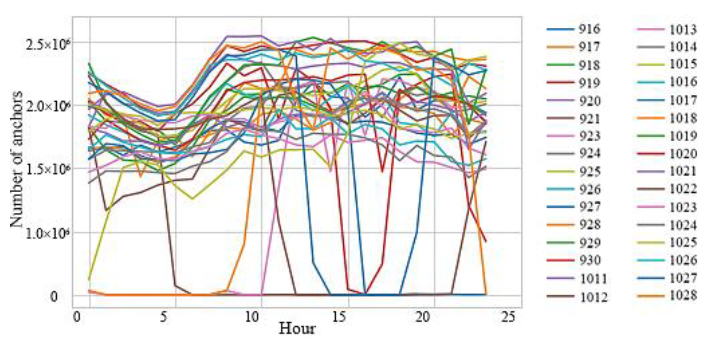
The GPS track data are categorized into days and hours according to the time field, and the changes in the number of positioning points are analyzed at different scales between the day and the time period. The time period characteristics for the number of location points are shown in Figure A1. The periods with many abnormal location points are 15–17 o’clock on 19 September 2011 and 6–24 o’clock on 21 September 2011.
Figure A1. Period characteristics of the number of anchor points.
Ijgi 11 00590 g0a1
(2)
Interday period characteristics of the number of vehicles
The GPS trajectory data are divided into days and hours according to the time field, the number of vehicles in different periods is counted separately, and the changes in the number of vehicles at different scales between days and periods are analyzed. The period characteristics for the number of vehicles are shown in Figure A2. As taxis are highly regulated by the government, the working hours of drivers are relatively fixed, and the number of vehicles each day varies little at different periods and only slightly decreases from 0–6 at night. It can be found that the lack of positioning points has much to do with the lack of vehicles.
Figure A2. Period characteristics of the number of vehicles.
Ijgi 11 00590 g0a2

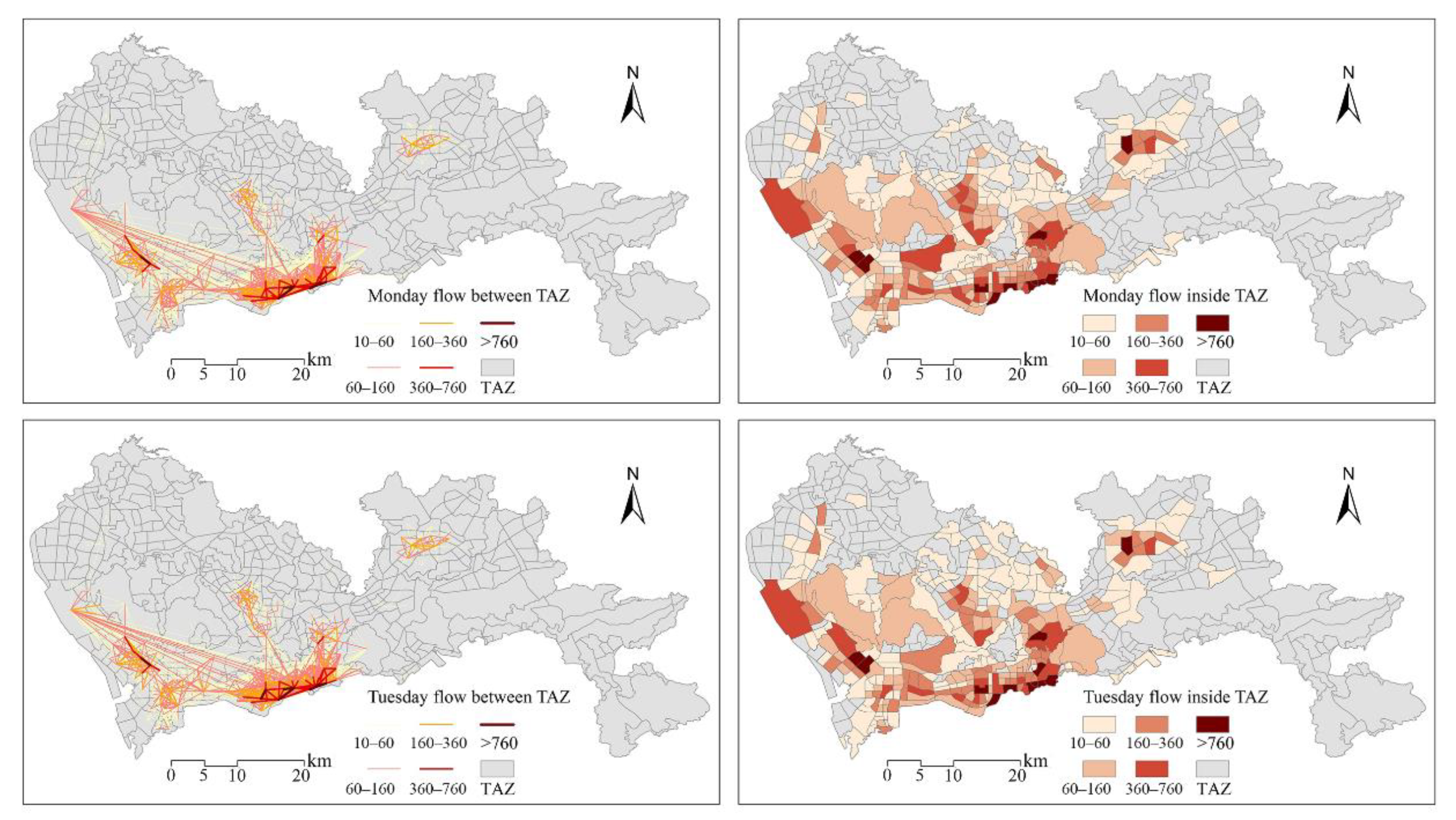
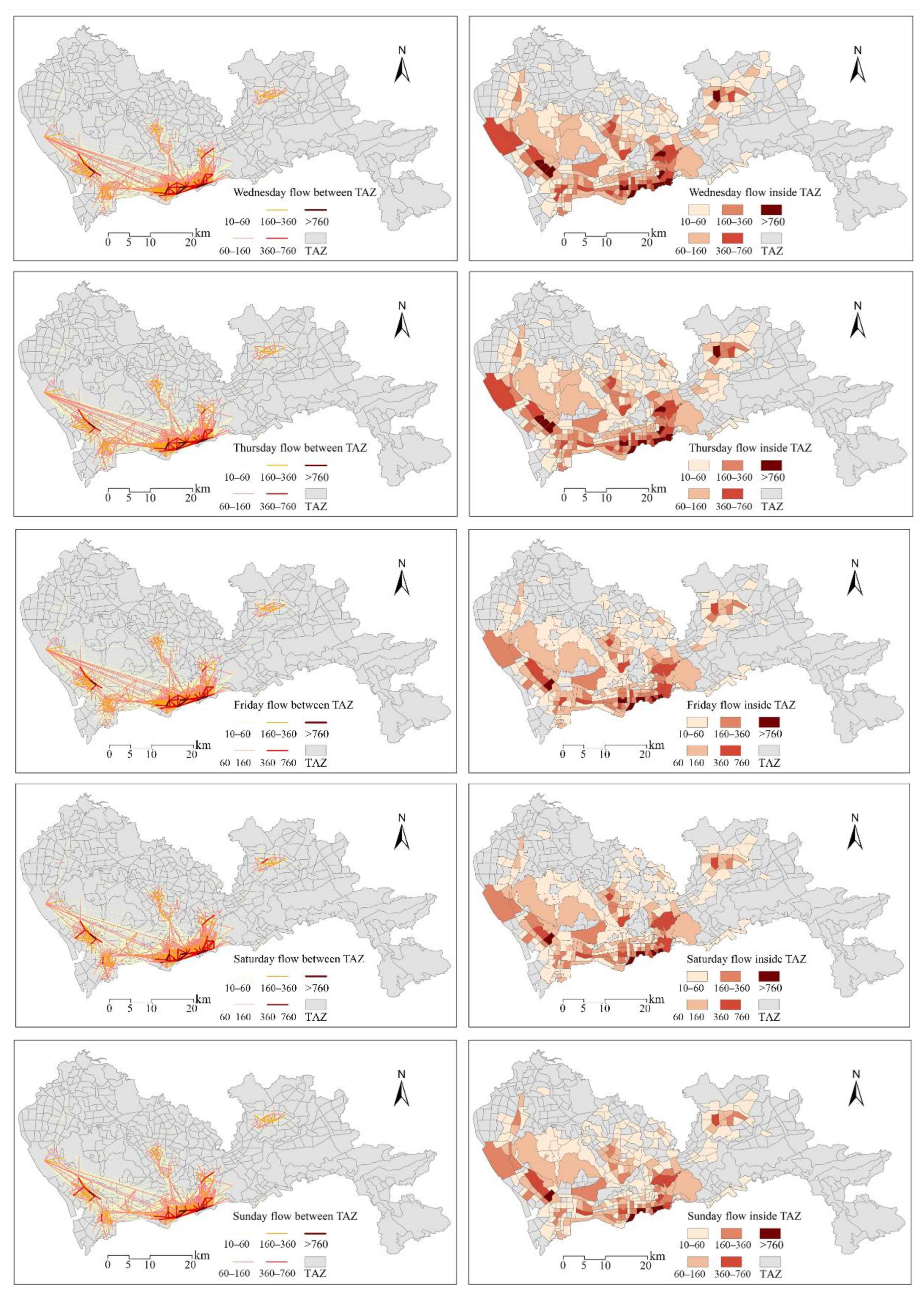
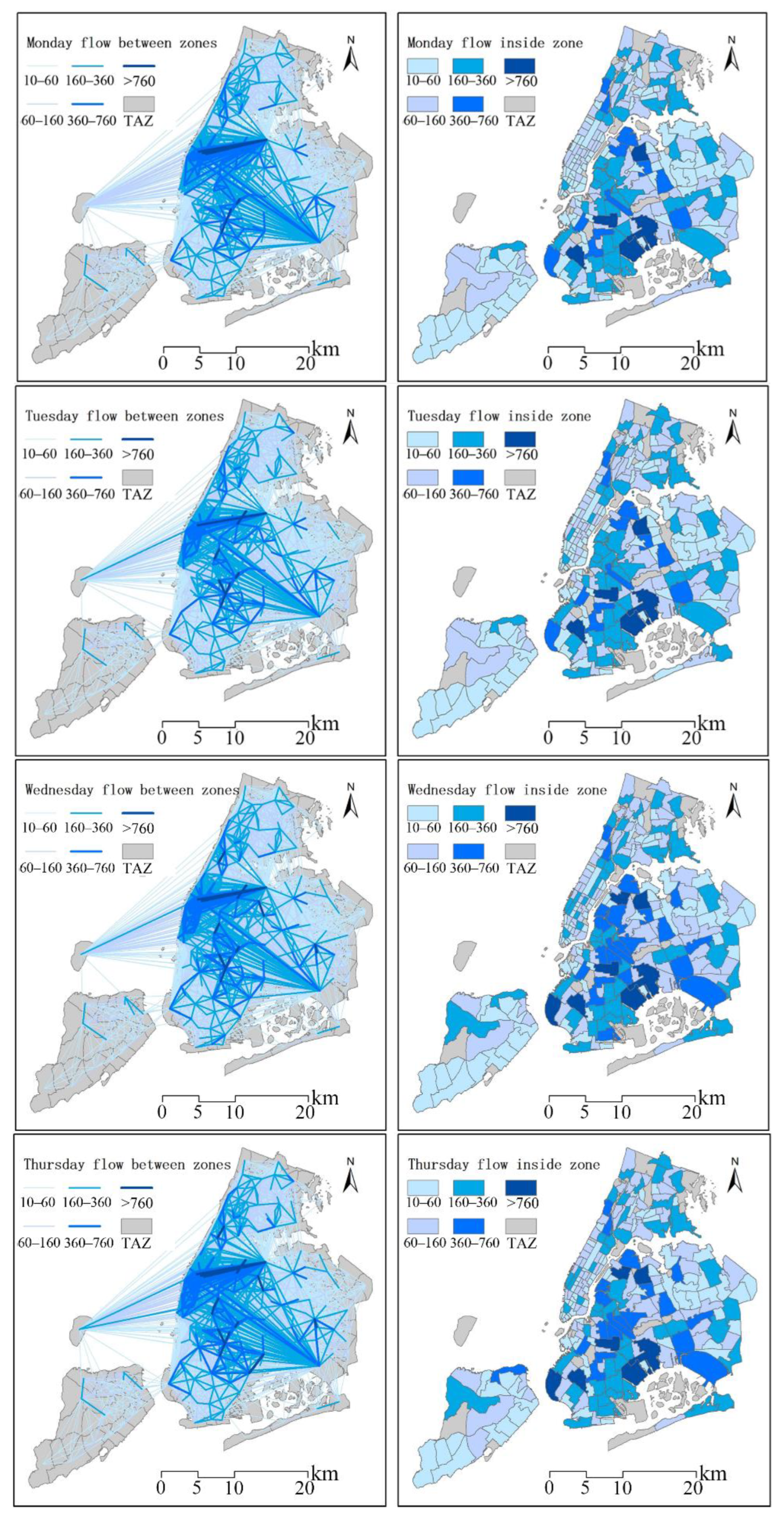
Appendix B. Daily OD Distribution

Based on the OD flow data on different days of the week, the travel flow between different units and within the units is calculated, and the results of Shenzhen are visualized as shown in Figure A3. The results of NYC are visualized as shown in Figure A4, which is a diagram of the travel spatial structure from Monday to Sunday (the left shows the flow of people between units, and the right shows the number of trips within units). You can intuitively see the difference in taxi travel patterns on different days and the more stable part of the taxi travel structure.
Figure A3. Travel spatial structure diagram from Monday through Sunday in Shenzhen.
Ijgi 11 00590 g0a3aIjgi 11 00590 g0a3b
Figure A4. Travel spatial structure diagram from Monday through Sunday in New York.
Ijgi 11 00590 g0a4aIjgi 11 00590 g0a4b
Through comparison and analysis of the above figures, it can be found that traveling by taxi is more biased toward short-distance travel. The high travel flows are mainly distributed between a single TAZ or between neighboring TAZs within a certain distance. These include the working area near Lingzhi Station in Baoan District, the Convention, and Exhibition Center Area, the Futian Port (Figure A5), the Science Museum area, near IT Technology Park (Figure A6), the Longhua Station Area, and the Ziwei Garden Area.
Figure A5. Trip flow diagram between and inside TAZs in Shenzhen.
Ijgi 11 00590 g0a5
Figure A6. Trip flow diagram between and inside TAZs in New York.
Ijgi 11 00590 g0a6

References

  1. Angrist, J.D.; Caldwell, S.; Hall, J.V. Uber versus taxi: A driver’s eye view. Am. Econ. J. Appl. Econ. 2021, 13, 272–308. [Google Scholar] [CrossRef]
  2. Bao, J.; Yang, Z.; Zeng, W.; Shi, X. Exploring the spatial impacts of human activities on urban traffic crashes using multi-source big data. J. Transp. Geogr. 2021, 94, 103118. [Google Scholar] [CrossRef]
  3. Behara, K.N.; Bhaskar, A.; Chung, E. A DBSCAN-based framework to mine travel patterns from origin-destination matrices: Proof-of-concept on proxy static OD from Brisbane. Transp. Res. Part C Emerg. Technol. 2021, 131, 103370. [Google Scholar] [CrossRef]
  4. Behara, K.; Bhaskar, A.; Chung, E. A novel approach for the structural comparison of origin-destination matrices: Levenshtein distance. Transp. Res. Part C Emerg. Technol. 2020, 111, 513–530. [Google Scholar] [CrossRef]
  5. Cai, H.; Zhan, X.; Zhu, J.; Jia, X.; Chiu, A.S.; Xu, M. Understanding taxi travel patterns. Phys. A Stat. Mech. its Appl. 2016, 457, 590–597. [Google Scholar] [CrossRef] [Green Version]
  6. Chen, F.; Yin, Z.; Ye, Y.; Sun, D. Taxi hailing choice behavior and economic benefit analysis of emission reduction based on multi-mode travel big data. Transp. Policy 2020, 97, 73–84. [Google Scholar] [CrossRef]
  7. Chen, X.; Xie, J.; Xiao, C.; Lu, B.; Shan, J. Recurrent origin–destination network for exploration of human periodic collective dynamics. Trans. GIS 2022, 26, 317–340. [Google Scholar] [CrossRef]
  8. Cheng, T.; Adepeju, M. Modifiable Temporal Unit Problem (MTUP) and Its Effect on Space-Time Cluster Detection. PLoS ONE 2014, 9, e100465. [Google Scholar] [CrossRef] [Green Version]
  9. Correa, D.; Xie, K.; Ozbay, K. Exploring the Taxi and Uber Demand in New York City: An Empirical Analysis and Spatial Modeling. In Proceedings of the 96th Annual Meeting of the Transportation Research Board, Washington, DC, USA, 8–12 January 2017. [Google Scholar]
  10. Fang, Z.; Su, R.; Huang, L. Understanding the Effect of an E-Hailing App Subsidy War on Taxicab Operation Zones. J. Adv. Transp. 2018, 2018, 7687852. [Google Scholar] [CrossRef]
  11. Gong, S.; Cartlidge, J.; Bai, R.; Yue, Y.; Li, Q.; Qiu, G. Geographical and temporal huff model calibration using taxi trajectory data. GeoInformatica 2021, 25, 485–512. [Google Scholar] [CrossRef]
  12. Guo, D.; Zhu, X.; Jin, H.; Gao, P.; Andris, C. Discovering Spatial Patterns in Origin-Destination Mobility Data. Trans. GIS 2012, 16, 411–429. [Google Scholar] [CrossRef]
  13. Guo, X.; Xu, Z.; Zhang, J.; Lu, J.; Zhang, H. An OD Flow Clustering Method Based on Vector Constraints: A Case Study for Beijing Taxi Origin-Destination Data. ISPRS Int. J. Geo-Inf. 2020, 9, 128. [Google Scholar] [CrossRef] [Green Version]
  14. Huang, J.; Zhang, Y.; Deng, M.; He, Z. Mining crowdsourced trajectory and geo-tagged data for spatial-semantic road map construction. Trans. GIS 2022, 26, 735–754. [Google Scholar] [CrossRef]
  15. Kou, Z.; Cai, H. Understanding bike sharing travel patterns: An analysis of trip data from eight cities. Phys. A Stat. Mech. Appl. 2019, 515, 785–797. [Google Scholar] [CrossRef]
  16. Lei, Y.; Ozbay, K. A robust analysis of the impacts of the stay-at-home policy on taxi and Citi Bike usage: A case study of Manhattan. Transp. Policy 2021, 110, 487–498. [Google Scholar] [CrossRef]
  17. Li, S.; Zhuang, C.; Tan, Z.; Gao, F.; Lai, Z.; Wu, Z. Inferring the trip purposes and uncovering spatio-temporal activity patterns from dockless shared bike dataset in Shenzhen, China. J. Transp. Geogr. 2021, 91, 102974. [Google Scholar] [CrossRef]
  18. Li, X.; Ma, X.; Wilson, B. Beyond absolute space: An exploration of relative and relational space in Shanghai using taxi trajectory data. J. Transp. Geogr. 2021, 93, 103076. [Google Scholar] [CrossRef]
  19. Li, X.; Pan, G.; Wu, Z.; Qi, G.; Li, S.; Zhang, D.; Zhang, W.; Wang, Z. Prediction of urban human mobility using large-scale taxi traces and its applications. Front. Comput. Sci. 2012, 6, 111–121. [Google Scholar] [CrossRef]
  20. Liu, X.; Gong, L.; Gong, Y.; Liu, Y. Revealing travel patterns and city structure with taxi trip data. J. Transp. Geogr. 2015, 43, 78–90. [Google Scholar] [CrossRef] [Green Version]
  21. Liu, Y.; Singleton, A.; Arribas-Bel, D.; Chen, M. Identifying and understanding road-constrained areas of interest (AOIs) through spatiotemporal taxi GPS data: A case study in New York City. Comput. Environ. Urban Syst. 2021, 86, 101592. [Google Scholar] [CrossRef]
  22. Liu, Y.; Wang, F.; Xiao, Y.; Gao, S. Urban land uses and traffic ‘source-sink areas’: Evidence from GPS-enabled taxi data in Shanghai. Landsc. Urban Plan. 2012, 106, 73–87. [Google Scholar] [CrossRef]
  23. Lyu, T.; Wang, P.; Gao, Y.; Wang, Y. Research on the big data of traditional taxi and online car-hailing: A systematic review. J. Traffic Transp. Eng. 2021, 8, 1–34. [Google Scholar] [CrossRef]
  24. Monahan, T.; Lamb, C.G. Transit’s downward spiral: Assessing the social-justice implications of ride-hailing platforms and COVID-19 for public transportation in the US. Cities 2022, 120, 103438. [Google Scholar] [CrossRef]
  25. Navarro, G. A guided tour to approximate string matching. ACM Comput. Surv. 2001, 33, 31–88. [Google Scholar] [CrossRef]
  26. Poongodi, M.; Malviya, M.; Kumar, C.; Hamdi, M.; Vijayakumar, V.; Nebhen, J.; Alyamani, H. New York City taxi trip duration prediction using MLP and XGBoost. Int. J. Syst. Assur. Eng. Manag. 2022, 13, 16–27. [Google Scholar] [CrossRef]
  27. Shehzad, K.; Bilgili, F.; Koçak, E.; Xiaoxing, L.; Ahmad, M. COVID-19 outbreak, lockdown, and air quality: Fresh insights from New York City. Environ. Sci. Pollut. Res. 2021, 28, 41149–41161. [Google Scholar] [CrossRef]
  28. Shenzhen Transportation Bureau. Passenger Flow Volume of Public Transport; Shenzhen Transportation Bureau: Shenzhen, China, 2021.
  29. Shu, H.; Pei, T.; Song, C.; Chen, X.; Guo, S.; Liu, Y.; Chen, J.; Wang, X.; Zhou, C. L-function of geographical flows. Int. J. Geogr. Inf. Sci. 2021, 35, 689–716. [Google Scholar] [CrossRef]
  30. Tu, W.; Cao, R.; Yue, Y.; Zhou, B.; Li, Q.; Li, Q. Spatial variations in urban public ridership derived from GPS trajectories and smart card data. J. Transp. Geogr. 2018, 69, 45–57. [Google Scholar] [CrossRef] [Green Version]
  31. Kumar, T.M.V. International Collaborative Research: “Smart Global Mega Cities” and Conclusions of Cities Case Studies Tokyo, New York, Mumbai, Hong Kong-Shenzhen, and Kolkata. In Smart Global Megacities; Springer: Singapore, 2022; pp. 411–460. [Google Scholar] [CrossRef]
  32. Wang, F.; Ross, C.L. New potential for multimodal connection: Exploring the relationship between taxi and transit in New York City (NYC). Transportation 2019, 46, 1051–1072. [Google Scholar] [CrossRef]
  33. Wang, H.; Zhang, K.; Chen, J.; Wang, Z.; Li, G.; Yang, Y. System dynamics model of taxi management in metropolises: Economic and environmental implications for Beijing. J. Environ. Manag. 2018, 213, 555–565. [Google Scholar] [CrossRef]
  34. Wang, J.; Rui, X.; Song, X.; Tan, X.; Wang, C.; Raghavan, V. A novel approach for generating routable road maps from vehicle GPS traces. Int. J. Geogr. Inf. Sci. 2015, 29, 69–91. [Google Scholar] [CrossRef]
  35. Li, Y.; Xiang, L.; Zhang, C.; Jiao, F.; Wu, C. A Guided Deep Learning Approach for Joint Road Extraction and Intersection Detection from RS Images and Taxi Trajectories. IEEE J. Sel. Top. Appl. Earth Obs. Remote Sens. 2021, 14, 8008–8018. [Google Scholar] [CrossRef]
  36. Yang, X.; Hou, L.; Guo, M.; Cao, Y.; Yang, M.; Tang, L. Road intersection identification from crowdsourced big trace data using Mask-RCNN. Trans. GIS 2022, 26, 278–296. [Google Scholar] [CrossRef]
  37. Zhang, D.; Wan, J.; He, Z.; Zhao, S.; Fan, K.; Park, S.O.; Jiang, Z. Identifying Region-Wide Functions Using Urban Taxicab Trajectories. ACM Trans. Embed. Comput. Syst. 2016, 15, 1–19. [Google Scholar] [CrossRef]
  38. Zhang, J.; Liu, X.; Senousi, A.M. A multilayer mobility network approach to inferring urban structures using shared mobility and taxi data. Trans. GIS 2021, 25, 2840–2865. [Google Scholar] [CrossRef]
  39. Zhang, S.; Tang, J.; Wang, H.; Wang, Y.; An, S. Revealing intra-urban travel patterns and service ranges from taxi trajectories. J. Transp. Geogr. 2017, 61, 72–86. [Google Scholar] [CrossRef]
  40. Zhang, Y.; Liu, J.; Qian, X.; Qiu, A.; Zhang, F. An Automatic Road Network Construction Method Using Massive GPS Trajectory Data. ISPRS Int. J. Geo-Inf. 2017, 6, 400. [Google Scholar] [CrossRef] [Green Version]
  41. Zhou, Y.; Fang, Z.; Thill, J.-C.; Li, Q.; Li, Y. Functionally critical locations in an urban transportation network: Identification and space–time analysis using taxi trajectories. Comput. Environ. Urban Syst. 2015, 52, 34–47. [Google Scholar] [CrossRef]
Figure 1. Travel spatial structure and travel flow of OD matrix. (a) Travel structrue of OD matrix. (b) Tavel flow of OD matrix.
Ijgi 11 00590 g001
Figure 2. Flow and variability classification method.
Ijgi 11 00590 g002
Figure 3. TAZs in Shenzhen.
Ijgi 11 00590 g003
Figure 4. TAZs in New York.
Ijgi 11 00590 g004
Figure 5. OD travel volume and distance per week. (a) Shenzhen City. (b) New York City.
Ijgi 11 00590 g005
Figure 6. Hourly OD travel volume. (a) Shenzhen City. (b) New York City.
Ijgi 11 00590 g006aIjgi 11 00590 g006b
Figure 7. Hourly OD distribution from Monday through Sunday. (a) Shenzhen City. (b) New York City.
Ijgi 11 00590 g007aIjgi 11 00590 g007b
Figure 8. Distribution of taxi travel flow volume. (a) OD proportion distribution in Shenzhen. (b) Volume proportion distribution in Shenzhen. (c) OD proportion distribution in New York. (d) Volume proportion distribution in New York.
Ijgi 11 00590 g008
Figure 9. The similarity changes with the threshold.
Ijgi 11 00590 g009
Figure 10. Normalized difference of OD volume. (a) Normalized difference between weekday and weekend in Shenzhen. (b) Normalized difference between weekend and weekday in Shenzhen. (c) Normalized difference between weekday and weekend in New York. (d) Normalized difference between weekend and weekday in New York.
Ijgi 11 00590 g010
Figure 11. Normalized difference of OD distribution. (a) Normalized difference between weekday and weekend of OD distribution in Shenzhen. (b) Normalized difference between weekend and weekday of OD distribution in Shenzhen. (c) Normalized difference between weekday and weekend of OD distribution in New York. (d) Normalized difference between weekend and weekday of OD distribution in New York.
Ijgi 11 00590 g011
Figure 12. Changes in the stability of the internal travel flow for geographic units. (a) Low travel flow on weekdays in Shenzhen. (b) High travel flow on weekdays in Shenzhen. (c) Low travel flow on weekends in Shenzhen. (d) High travel flow on weekends in Shenzhen. (e) Low travel flow on weekdays in New York. (f) High travel flow on weekdays in New York. (g) Low travel flow on weekends in New York. (h) High travel flow on weekends in New York.
Ijgi 11 00590 g012aIjgi 11 00590 g012b
Figure 13. Changes in the stability of taxi travel flow for geographic units. (a) Low travel flow on weekdays in Shenzhen. (b) High travel flow on weekdays in Shenzhen. (c) Low travel flow on weekends in Shenzhen. (d) High travel flow on weekends in Shenzhen. (e) Low travel flow on weekdays in New York. (f) High travel flow on weekdays in New York. (g) Low travel flow on weekends in New York. (h) High travel flow on weekends in New York.
Ijgi 11 00590 g013aIjgi 11 00590 g013b
Figure 14. The degree of travel spatial structure and flow recovery. (a) Travel spatial structure in Shenzhen. (b) Travel spatial structure in NYC. (c) Travel spatial flow in Shenzhen. (d) Travel spatial flow in NYC.
Ijgi 11 00590 g014
Figure 15. The degree of representation of high- and low-travel structures and flows. (a) Travel spatial structure in Shenzhen. (b) Travel spatial structure in New York. (c) Travel flow in Shenzhen. (d) Travel flow in New York.
Ijgi 11 00590 g015aIjgi 11 00590 g015b
Table 1. Sample records of a GPS trajectory in Shenzhen.
Device NumberLongitudeLatitudePositioning TimeWorking Status
104***3113.****0522.****1826 September 2011 11:18:550
104***3113.****4922.****0726 September 2011 11:19:321
104***3113.****3222.****5626 September 2011 11:20:021
104***3113.****0722.****9526 September 2011 11:21:001
Table 2. Trip records of High Volume For-Hire Vehicle in New York City.
PickUp_DatetimeDropOff_DatetimePULocationIDDPLocationID
1 July 2019 00:12:331 July 2019 00:25:0022889
1 July 2019 00:41:261 July 2019 00:51:2197188
1 July 2019 00:18:501 July 2019 00:32:4881220
1 July 2019 00:29:011 July 2019 00:45:5069239
Table 3. Structural similarity of the OD matrixes in Shenzhen.
Structural SimilarityMondayTuesdayWednesdayThursdayFridaySaturdaySunday
Monday1.0000.8100.8080.8110.8040.7960.793
Tuesday0.8101.0000.8080.8090.8060.8020.801
Wednesday0.8080.8081.0000.8100.8120.8020.798
Thursday0.8110.8090.8101.0000.8130.8010.801
Friday0.8040.8060.8120.8131.0000.8060.802
Saturday0.7960.8020.8020.8010.8061.0000.806
Sunday0.7930.8010.7980.8010.8020.8061.000
Table 4. Flow similarity of the OD matrixes in Shenzhen.
Structural SimilarityMondayTuesdayWednesdayThursdayFridaySaturdaySunday
Monday1.0000.7400.7320.7350.7240.7120.709
Tuesday0.7401.0000.7350.7330.7300.7230.719
Wednesday0.7320.7351.0000.7430.7430.7210.716
Thursday0.7350.7330.7431.0000.7410.7210.717
Friday0.7240.7300.7430.7411.0000.7290.721
Saturday0.7120.7230.7210.7210.7291.0000.734
Sunday0.7090.7190.7160.7170.7210.7341.000
Table 5. Structural similarity of the OD matrixes in New York.
Structural SimilarityMondayTuesdayWednesdayThursdayFridaySaturdaySunday
Monday1.0000.5670.5670.5670.5640.5650.562
Tuesday0.5671.0000.5680.5670.5650.5660.563
Wednesday0.5670.5681.0000.5690.5670.5660.563
Thursday0.5670.5670.5691.0000.5650.5630.561
Friday0.5640.5650.5670.5651.0000.5590.559
Saturday0.5650.5660.5660.5630.5591.0000.558
Sunday0.5620.5630.5630.5610.5590.5581.000
Table 6. Flow similarity of the OD matrixes in New York.
Structural SimilarityMondayTuesdayWednesdayThursdayFridaySaturdaySunday
Monday1.0000.5900.5760.5760.5380.4620.489
Tuesday0.5901.0000.5990.5870.5430.4590.481
Wednesday0.5760.5991.0000.5950.5570.4700.487
Thursday0.5760.5870.5951.0000.5730.4840.498
Friday0.5380.5430.5570.5731.0000.5170.513
Saturday0.4620.4590.4700.4840.5171.0000.530
Sunday0.4890.4810.4870.4980.5130.5301.000
Publisher’s Note: MDPI stays neutral with regard to jurisdictional claims in published maps and institutional affiliations.

