Article

Ship Target Recognition Based on Context-Enhanced Trajectory

Institute of Information Fusion, Naval Aviation University, Yantai 264001, China
*
Author to whom correspondence should be addressed.
ISPRS Int. J. Geo-Inf. 2022, 11(12), 584; https://doi.org/10.3390/ijgi11120584
Submission received: 28 August 2022 / Revised: 8 November 2022 / Accepted: 20 November 2022 / Published: 23 November 2022

Abstract

:
Ship target recognition based on trajectories has great potential in the field of target recognition. In the existing research, the context information is ignored, which limits the improvement of ship target recognition ability. In addition, the process of trajectory feature extraction is complex, and recognition accuracy needs to be further improved. In this paper, a ship target recognition method based on a context-enhanced trajectory is proposed. The maritime context knowledge base is constructed to enhance the trajectory information and to improve the separability of different types of target trajectories. A deep learning model is used to extract trajectory features and context features automatically. Offline training and online recognition are adopted to complete the target recognition task. Experimental analysis and verification are carried out using the automatic identification system (AIS) dataset. The recognition accuracy increases by 7.91% after context enhancement, which shows that the context enhancement is efficient. The proposed method also has a strong anti-noise ability. In the noisy environment set in this paper, the recognition accuracy of the proposed method is still maintained at 86.13%.

1. Introduction

Most studies have recognized ship targets by utilizing optical imaging [1,2] and radar information [3,4,5,6]. However, target trajectories contain rich motion characteristics [7]; therefore, target recognition based on trajectories is an important research direction in the field of target recognition and has great research potential. Feature extraction is an important step of target recognition. There are two main ways to extract the features: handcrafting and learning. Handcrafted features usually include speed characteristics and steering characteristics [8,9,10]. According to experience, some statistical characteristic features are designed to distinguish different types of targets. Feature learning is a technique of deep learning. The neural network is designed to learn the trajectory data and obtain the feature representation [11,12].
However, when the differences in motion features among different targets are not significant, it will be difficult to recognize the target only by trajectories. In the research of ship target recognition by trajectory, the use of context information is lacking. The background of the target’s geographic location is not blank. The targets have different background information in different spatiotemporal locations, which adds context attributes to the target’s trajectories. For example, the trajectories of ocean-going freighters often appear in the deep sea, while the trajectories of small speedboats are more distributed in nearshore waters. Mining rules in the context information of different ship targets and applying them to target recognition can enhance the trajectory information. Therefore, the trajectories among different types of targets are more discriminative, thus recognizing the target type more accurately. In the research of land target recognition based on trajectory, researchers have attempted to add context knowledge into the decision information as a way to improve the model’s ability. In the research of land target recognition by trajectory, context information is used as a kind of auxiliary information to improve the recognition ability. Good results have been achieved. One study [13] extracted characteristic information about a station. Another study [14] analyzed information about stops at important locations. Another study [15] introduced context information such as the type of land, slope, altitude, temperature, and humidity when performing similarity measurements of hurricane trajectories. When analyzing the trajectories of two tigers, one study [16] considered some contextual factors: slope, vegetation density, prey density, and proximity to the boundary. However, different from land, there are no numerous landmark buildings on the sea, there are no fixed road constraints, and the sea background is simple. Therefore, it is difficult to apply the above methods directly to sea trajectory analysis.
In view of the above problems, this paper constructs a context knowledge base from the aspects of maritime traffic density, distance of target to shore, and distance of target to port to enhance trajectory information. On this basis, features in trajectory information and context information are extracted using the transformer and long short-term memory (LSTM) models, respectively. Then, the features are fused to obtain comprehensive feature vectors to achieve more accurate recognition of the target. This paper is organized as follows. Section 2 presents a review of related studies. Section 3 provides the problem description. Section 4 presents our proposed method. Section 5 shows the dataset preparation. Section 6 displays the experiments and analysis. Section 7 draws some conclusions.

2. State-of-the-Art Review

The trajectory consists of points generated by the target over a period of time, and the trajectory points follow a time order. The trajectory is a typical time series [17]. Therefore, target recognition based on trajectories is a time series classification problem (TSC). There have been extensive studies on TSC. However, they could not capture the motion characteristics of the trajectories. One study [18] proposed a method based on distance measurement, which adopted dynamic time warping (DTW) to measure the similarity between time series. Another study [19] showed a shapelet transformation method, which transformed the time series into other spaces; therefore, the different kinds of time series were more separable. One study [17] attempted to combine 35 classifiers to improve the classification ability of the model. They did not consider the motion features of targets in the process of classification. For the concrete task of trajectory series classification, researchers have given more attention to the motion characteristics of the target. The main idea is to extract the motion characteristics of the trajectory series and then classify the trajectories. The trajectory is a multidimensional sequence that provides rich information for motion feature extraction. The trajectories generated by different target types usually have different motion characteristics. For example, the speed of a speed boat is often higher than that of a freighter, and its maneuverability is also higher than that of the freighter. One study [8] used the fuzzy logic algorithm to predict the types of targets according to the trajectories. The target types were classified into “wanted” and “unwanted”, which is a binary classification problem. However, there were too few member functions in the paper to handle more complex recognition tasks. In another study [9], more trajectory attributes were considered; therefore, more member functions were added to improve the recognition ability of the model. Fuzzy logic algorithms have been widely used [20,21,22], but the determination of member functions requires not only profound professional knowledge but also rich experience. One study [10] used a support vector machine (SVM) to classify trajectories, which verified the effectiveness of machine learning in solving the problem of target recognition based on trajectories. Another study [23] extracted more features for the SVM. Another study [24] proposed a Gaussian mixture model to distinguish flight trajectories from non-flight trajectories. However, the ratio of the two types of trajectories is required as the prior information, which is not applicable to practical applications. Another study [25] proposed three motion patterns of the trajectories and then extracted the features of the three motion patterns. The division of the three motion patterns is helpful in extracting the features of the trajectories in different motion states. However, the process of motion pattern classification and feature extraction is complicated. In one study [26], an automatic feature extractor was designed. Principal component analysis (PCA) was used to analyze the extracted features, and then many machine learning classifications were adopted to achieve classification. Although machine learning methods perform well, the design and analysis of statistical features are complex. Some researchers have attempted to use deep learning methods. One study [11] designed a recurrent neural network (RNN) to recognize ship types, and another [12] used a multilayer perceptron (MLP) to recognize cargo ships, fishing boats, and passenger ships. This study verified the feasibility of deep learning methods in solving this problem.
There are two types of geographic information systems (GISs): transaction processing systems and decision support systems [27]. In this paper, geographic information is used as a kind of decision-support information, which helps to recognize ships in the maritime environment. In maritime traffic, GIS is usually applied to support maritime surveillance. In one study [28], GIS was used to analyze the spatial patterns of maritime accidents to improve maritime traffic management. Another study [29] combined GIS and multicriteria decision-making to assess and map maritime transportation risk. GIS is meaningful for providing information in the decision-making process. How to apply GIS to various maritime tasks is a promising research direction.

3. Problem Description

The target is usually in a certain context and constrained by it; therefore, the accuracy of target recognition can be improved by enhancing the context of the trajectory information. The context-enhanced trajectory can be expressed as {T;C}, where T represents trajectory information and C represents context information. The target type is y, and ship target recognition based on the context-enhanced trajectory obtains y from{T;C}.
The trajectory is a record of a target’s positions over a period of time. The trajectory data obtained at a certain sampling interval are a discrete multidimensional sequence, which follows the logical order of time. The data dimension of each time step is equal, and each dimension represents an attribute of the trajectory point. The trajectory can be expressed as:
T i = { P i 1 , , P i j , , P i n } ,   j [ 1 , n ]
where T i represents the i th trajectory in the trajectory dataset T. n is the total number of trajectory points in trajectory T i . P i j represents the j th trajectory point in trajectory T i . Each trajectory point contains five dimensions of information, including latitude (lat), longitude (lon), speed over ground (sog), course over ground (cog), and timestamp (t), which can be expressed as:
P i j = ( l a t , l o n , s o g , c o g , t )
The context information C is the information related to the geographic environment. Different geographic environments have different information, which provides additional information about the location of the target, not just a position coordinate. The difficulty lies in transforming context information into numerical information. To transform the context information, some basic formulas are used. For example, the distance between two points is:
d = ( l o n 1 l o n 2 ) 2 + ( l a t 1 l a t 2 ) 2
The Euclidean distance is used to approximate the distance between two points on the sea surface because the application scenario is usually a small piece of sea for a specific task. The density formula is also used:
m = n p a
where n p is the number of trajectory points in a certain grid and a is the area of the grid. The details of the context knowledge base are presented in Section 4.2. A concrete application example is given in Section 5.2.

4. Approach

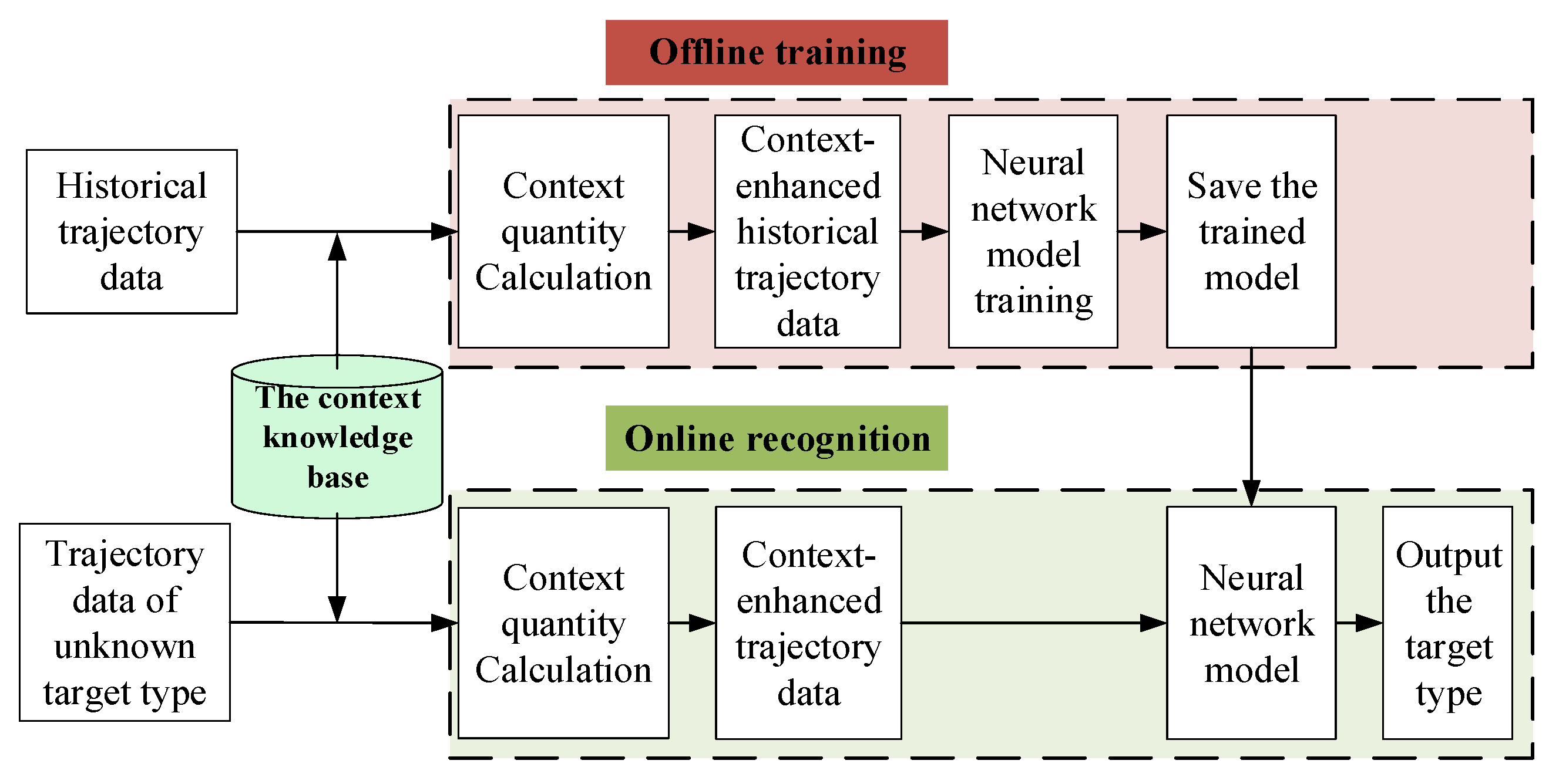
4.1. The Overall Process

As shown in Figure 1, the overall process of the proposed method is divided into two parts: the first part is offline training, and the second part is online recognition. The purpose of offline training is to obtain the network model that can be used to recognize the target. Online recognition recognizes the target category according to the trajectory of the unknown target type. For the offline training part, first, the context knowledge corresponding to the trajectory is calculated according to the historical trajectory dataset and context knowledge base. The historical trajectory dataset after the context enhancement is obtained. Then, the neural network is built and trained with the historical trajectory dataset above. Finally, we save the trained neural network model. For the online recognition part, first, according to the trajectory information, the information of the context knowledge base is called to calculate the context knowledge corresponding to the trajectory. The context-enhanced trajectory data to be recognized are obtained. Second, the neural network model trained in the offline training process is called, and the context-enhanced trajectory is input into the network model. Finally, the target category is output. The task of online target category recognition is completed.
The characteristics of the proposed method are in line with the actual situation. Offline training needs to collect a historical dataset, build a context knowledge base, and train the model. The training process consumes much time, occupies considerable computing power, and has a high hardware configuration. The online recognition part has lower requirements on time consumption, computing power consumption, and hardware configuration.

4.2. Context Knowledge Base

The sea area through which the target passes has context knowledge. The context information in different geographic locations is different. To distinguish the characteristic difference between different types of targets more effectively, we use context knowledge to enhance the trajectory information. Figure 2 shows the thermal maps of active areas for different types of ships. Figure 2a is the thermal map over the entire area. Figure 2b shows the details of the thermal map. The data used are described in Section 4. There are nine types of ships: fishing, military ops, SAR (search and rescue), tug, passenger, cargo, tanker, pleasure craft, and other ships. The red parts represent the area where the ships appear frequently, and the darker the color, the more frequently the target appears in the area. There are differences in the areas where ships of different types frequently appear, which can be used to help distinguish between different types of ships. Specifically, there are differences in the distance to the coast in areas where different types of ships frequently appear. In addition, the density of traffic varies in different areas. Three types of context information are extracted: maritime traffic density, distance of target to shore, and distance of target to ports. The following is an analysis of this contextual information.
This research focuses on identifying the real type of target using trajectory and context information. It does not involve tracking problems, assuming that the target has been stably tracked beforehand.

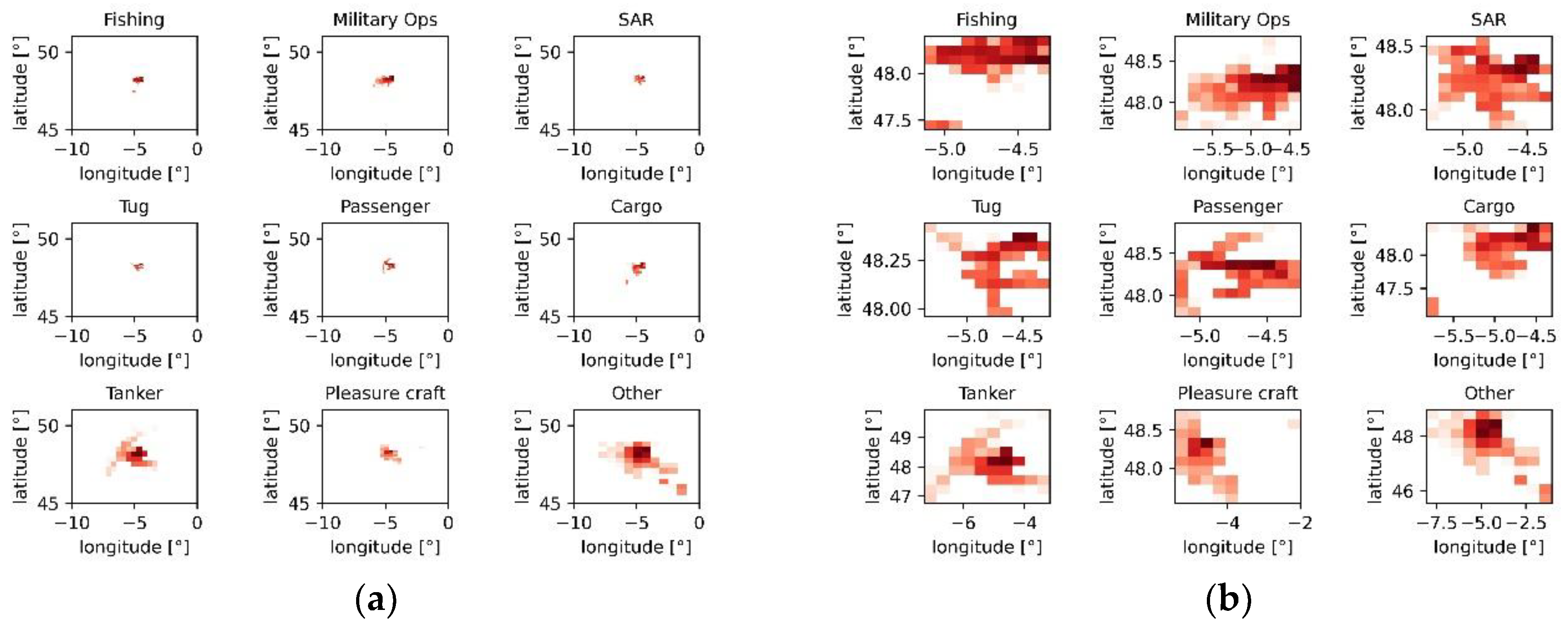
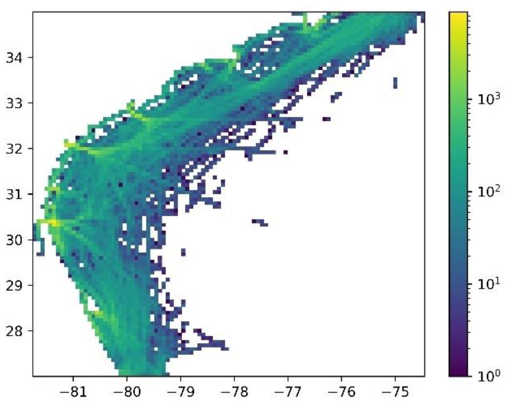
4.2.1. Maritime Traffic Density

The density of maritime traffic reflects the density of passing ships in the sea area in the historical data. The traffic density in the sea area with frequent occurrence of different types of targets is different. We use a neural network to learn its rules and provide the basis for target recognition. First, the sea area is subdivided into identical grids, and the traffic density in the historical data in each grid is calculated by the following formula:
t d i = n i a
where t d i represents the maritime traffic density of the i th grid. n i is the number of ships in the i th grid. a represents the area of the grid. After the grid map of maritime traffic density is obtained, the grid corresponding to each point in the trajectory can be determined by the latitude and longitude. Then, the density of maritime traffic at each trajectory point is obtained. By arranging the maritime traffic density at each trajectory point in the time order, the first context information of the target trajectory can be obtained:
t d = [ t d 1 , t d 2 , t d 3 , , t d n ]

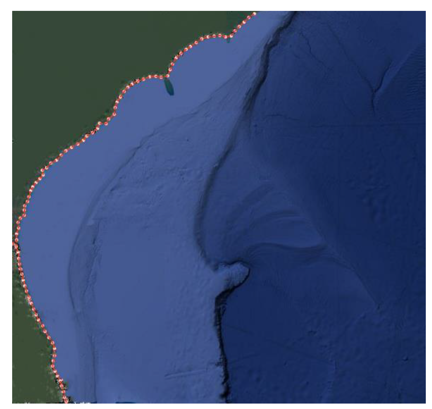
4.2.2. Distance from Target to Shore

The tasks performed by different types of ships depend on the nature of the ships. Some ships often go on ocean voyages, while others often appear in nearshore waters. The distance from the shore of a ship’s trajectory will show patterns in historical data, which can be used to recognize unknown ships. The distance of each point in the trajectory to shore is arranged in time order. We obtain the second context information:
d s = [ d s 1 , d s 2 , d s 3 , , d s n ]

4.2.3. Distances from Target to Ports

Ships do not navigate the ocean in random directions. Their route planning is mission-driven, showing that they are going from one port to another. Although there will be situations such as avoidance, anchoring, and rest, the overall sailing process is purpose-oriented. Therefore, the context information regarding the ship’s port of departure and port of destination can be used as a feature for the recognition of unknown targets. However, in the real world, it is difficult to obtain the whole trajectory of the target from the departure port to the destination port. Therefore, we cannot directly obtain the departure port and destination port information. However, the distances from the trajectory point to each major port are easy to obtain. By calculating the distances between each trajectory’s point and each major port, we obtain the distance matrix:
d p = [ d p 11 d p 12 d p 13 d p 1 m d p 21 d p 22 d p 23 d p 2 m d p 31 d p 32 d p 33 d p 3 m d p n 1 d p n 2 d p n 3 d p n m ]
where m represents the number of ports and n represents the number of points in a trajectory. In the course of sailing, the distance between the ship and departure port increases, and the distance between the ship and destination port decreases, which is reflected in the distance matrix. For example, we assume that the destination port is Port 1 and the destination port is Port 2. Then, the first column of dp generally shows a trend of increasing, and the second column generally shows a trend of decreasing. The information of the departure port and destination port of the target is transformed into a matrix, which not only transforms the information into standardized data but also solves the problem in which it is difficult to obtain the destination port and destination port directly. In this paper, the distance matrix dp is taken as the third type of context information, and the end-to-end learning ability of deep learning is utilized to automatically extract features to distinguish different types of targets.

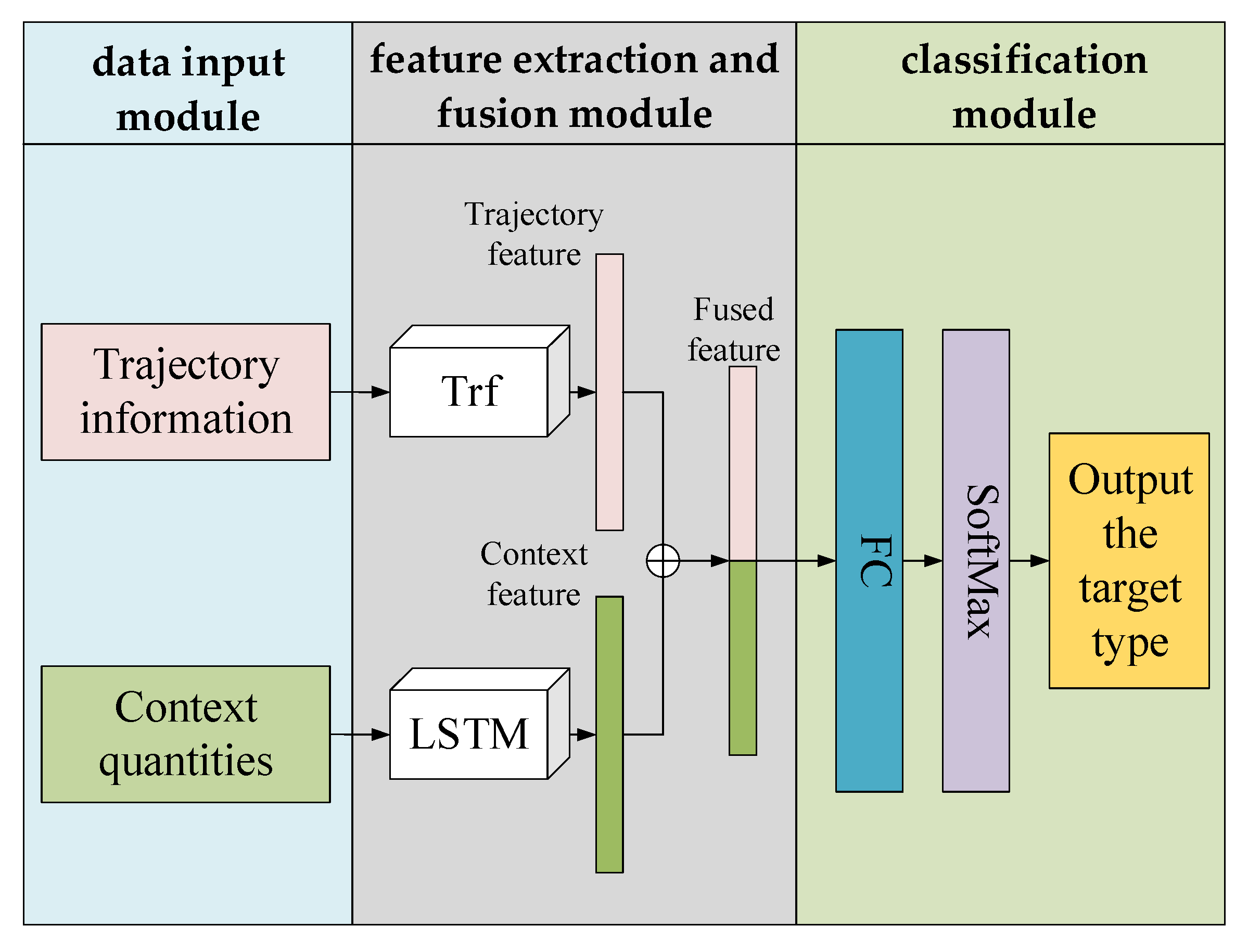
4.3. Neural Network Model

Figure 3 shows the structure of the neural network model. It includes three modules: a data input module, a feature extraction and fusion module, and a classification module. The trajectory information and context information depict the different attributes of the target. The main idea is to fuse the two kinds of information, obtain the fused information, and use the fused information to identify the target. Information fusion is a critical step. Trajectory information and context information are of different types; therefore, it is difficult to integrate them directly. The deep learning method provides a feature-level fusion method. One study [30] used two networks to extract the features of image information and text information, and the features were fused to obtain a fusion feature representation. Another study [31] first extracted the global feature and local feature of images and then fused them in the feature space. In our research, by using the feature extraction network, the trajectory information and context information are transformed into the feature space, and the feature vector is obtained. The feature vector is a unified representation. The feature vectors are used to realize the fusion of two kinds of information, which is the feature-level fusion. Specifically, the fusion feature is obtained by the concatenation operation in the feature space. By training the network model, in the feature space, the fusion features of different targets are far away from each other, and the fusion features of the same type of targets are close to each other to achieve the classification of targets. First, the data input module reads the formatted data. Second, the feature extraction and fusion module extracts the features of the trajectory information and the context information and fuses the extracted features to obtain the fused features. Finally, the fully connected layer and SoftMax layer complete the classification of the trajectory and output the category of the target. The format of the input data is M × L × D, where M represents the number of samples in one batch during the training process. L represents the length of a trajectory sample, which is the number of points in a trajectory. D is the dimension of each trajectory point. The transformer neural network was first proposed by Vaswani A. et al. in a study [32]. They used it to solve machine translation tasks and realize the processing of sequence data. The multihead attention algorithm was applied internally, which had advantages in extracting potential features. Multihead attention could effectively consider the important features of the trajectory, improving the attention to beneficial information and suppressing irrelevant information. Thus, the feature vectors extracted were more discriminative. Context information has a large dimension, and the rules of its change are easy to understand and mine. A LSTM [33] was used to extract feature information from context information. LSTM has a small number of structural parameters and easily converges.

5. Data Preparation

This paper adopts the automatic identification system (AIS) data of a certain sea area in Europe for analysis and verification. We construct a context knowledge base in this area. The AIS data include the position and motion information. The target types are also recorded, which can be set as the label to train and test our neural network model. The European automatic identification system (AIS) dataset is set for maritime-related applications. The navigation information of ships for six months, from 1 October 2015 to 31 March 2016, is recorded. The location covers the Celtic Sea and the Bay of Biscay (France). It contains more than 19 million AIS records. Nine main ship types are selected from the European AIS data: fishing, military ops, SAR (search and rescue), tug, passenger, cargo, tanker, pleasure craft, and other ships. The data are divided into a training set and a test set, 80% of which is the training set and the remaining 20% is the test set. Each type of ship has 864,000 AIS records. The network model is trained by the training set, and the recognition ability of the network model is tested on the test set.

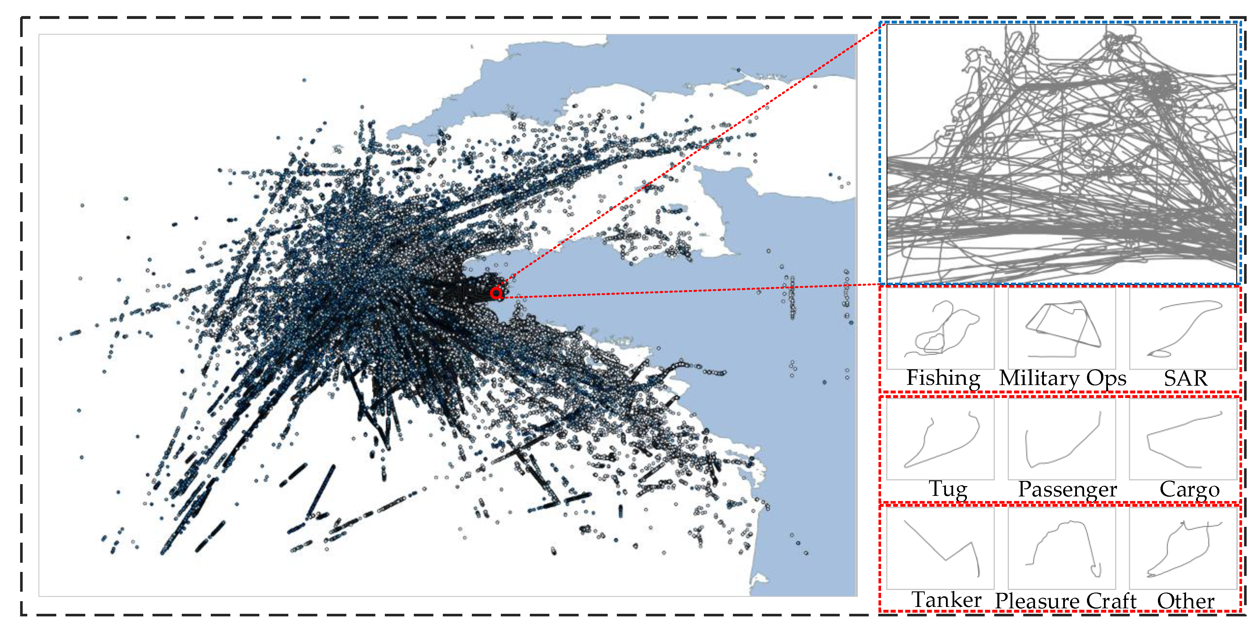
5.1. Trajectory Data Preprocessing

The original data in the AIS are unordered and contain redundant information. First, we sort the data according to the order of target type, MMSI (maritime mobile service identity identification), and time stamp. Then, the redundant information is removed, leaving only the timestamp, latitude, longitude, speed, heading, and target type information of the trajectory. The target type is converted into a label value, and the numbers 0–8 represent the 9 types of targets, respectively.

5.2. Context Knowledge Base Construction and Context Quantity Calculation

The construction of a context knowledge base prepares for calculating the context quantity corresponding to the trajectory. Construction is the process of extracting the trajectory’s background, and the calculation of the corresponding context quantity of each trajectory is the process of quantifying the context background. The whole step realizes the transformation of qualitative context background knowledge into input data that can be quantitatively calculated by the neural network model.
The AIS data used in this experiment are from the Celtic Sea and the Bay of Biscay (France) (see Figure 4). In Figure 4, the white part represents the sea, the blue part represents the land, and the points represent the trajectory points. The trajectories in the blue part are from rivers and lakes on land. Because this study only focuses on targets in the sea area, tracks in the inland area are excluded in the subsequent data cleaning and track sample generation. The right half of Figure 4 shows the enlarged partial detail and the trajectories of ship types. We take the construction of a context knowledge base in this sea area as an example to introduce the process of each context knowledge construction and the way of calculating context quantities through the knowledge base (The link to data and figure is https://zenodo.org/record/1167595/files/%5BP1%5D%20AIS%20Data.zip?download=1.) (accessed on 16 October 2021).

5.2.1. Maritime Traffic Density (td)

The maritime traffic density grid is constructed by using AIS historical data, and the sea area is divided into equal square grids. The map contains a total of 10,000 grids, with 100 grids per row and 100 grids per column. The physical size of the unit grid is 4.8 × 4.38 . The trajectory point density of each grid is calculated as the traffic density of this grid to obtain the grid map of maritime traffic density. Each grid contains two attributes: grid number and grid value. Figure 5 shows the grid graph drawn after calculation. The color changes gradually from purple to yellow as the value in the grid increases, which intuitively reflects the traffic density at different locations in this sea area. After the knowledge base of maritime traffic density is established, the corresponding context quantity td can be calculated for the trajectory sample. First, the grid number i of the trajectory point is queried according to the longitude and latitude information, and the grid value t d i is obtained. Then, the t d i for each point is obtained. The t d = [ t d 1 , t d 2 , t d 3 , , t d n ] is formed.

5.2.2. Distance from Target to Shore (ds)

The real coastline is very tortuous and can be regarded as an irregular combination of convex polygons and concave polygons. It is difficult to calculate the precise distance from the target to the shore. The task does not need to obtain an accurate distance. The context knowledge only needs to reflect whether the target is near or far from shore. Accordingly, a general approximate distance calculation method is proposed in this paper, which can be used in building context knowledge bases in different regions. First, we mark points along the coastline at intervals. The interval of marker points depends on the distance between historical trajectory data and the coast. If they are generally far from the coast, the interval of marker points increases; otherwise, it decreases. After the whole coastline is marked, several marker points are obtained. Figure 6 shows the markers (white points) on the coastline. We calculate the distance between the target and each marker point. The minimum distance is the approximate distance between the target and the coastline. The work of marking is the knowledge base-building process. The process of calculating the approximate distance according to marker points is the process of obtaining d s = [ d s 1 , d s 2 , d s 3 , , d s n ] .

5.2.3. Distances from Target to Ports

First, we select the major ports along the coast and record their latitude and longitude. Then, the distance between the target and each port is calculated by the longitude and latitude. The first step is the process of establishing the knowledge base of distances from target to ports. The second step is the process of obtaining dp. In this experiment, the parameters n and m are 30 and 20, respectively. Since the identification task usually focuses on ships in a certain part of the ocean, the number of ports is not large. However, the origin or destination port may be outside the map segment. In this kind of scenario, the selected ports could not provide such comprehensive context information. Context information is a kind of auxiliary information to enhance the trajectory information, the purpose of which is to improve the recognition ability of targets. It cannot be used as primary identifying information. Indeed, the more comprehensive the context information is, the more helpful it is to improve the recognition ability. However, the lack of comprehensive situational information will not make the model unable to converge because the trajectory information occupies a dominant position. However, the lack of comprehensive situational information can limit the improvement of the recognition ability. How to obtain more comprehensive information is worth further research.

5.3. Normalization

Neural networks are very sensitive to singular values and different distributions of data dimensions during training. To avoid such adverse effects, 0–1 normalization is used to normalize the data:
x i j = x i j x min x max x min
where x represents one dimension of the j th point in the i th trajectory. x max = max i [ 1 , m ] , j [ 1 , n ] x i j , x min = min i [ 1 , m ] , j [ 1 , n ] x i j . More specifically, all data that are fed into the network model are normalized. The maximum and minimum values in Formula (9) are derived from the already observed data; however, in addition to the data observed in this experiment, larger or smaller values may appear. In this case, the maximum and minimum values in Formula (9) should include the new observations when regularizing the new data.

6. Experiments and Discussion

In this section, two groups of experiments are designed to verify the effectiveness of the context enhancement, the superiority of the model over other algorithms, and the anti-noise ability. The dataset constructed in Section 5 is used for the experiments. All experiments are implemented under the PyTorch deep learning framework on a 64-bit station with Ubuntu 20.04.2, 16 GB of RAM, 8 Intel(R) Core (TM) i7-9700 CPU, and NVIDIA RTX 2080Ti.

6.1. Validation of Context Enhancement

In this group of experiments, the effectiveness of context enhancement is verified. The accuracy is selected as the experimental index. Three sub-experiments are set for comparison. The input data of the three sub-experiments are trajectory information without context enhancement, trajectory information after context enhancement, and only context information. The three sub-experiments are numbered I, II, and III. The accuracies of Experiment I and Experiment II on the test dataset are 89.32% and 97.13%, respectively. Figure 7a,b shows the confusion matrices of the results. Comparing Experiment I and Experiment II, the recognition accuracy increases by 7.91% after context enhancement. The results show that the ability of target recognition can be improved by enhancing the context information of the trajectory. Furthermore, to prove the effectiveness of the fusion of trajectory features and context features, we set Experiment III. The accuracy of Experiment III is 48.85%. Figure 7c shows the confusion matrix. Then, we number the trajectory samples in the experiment. We save the sample numbers that are correctly identified and incorrectly identified in Experiment I. We also do the same for Experiment III. According to the analysis of the numbers recorded above, for Experiment I, the proportion of misidentified samples is 10.68%. A total of 35.45% of the misidentified samples in Experiment I are correctly identified in Experiment III, accounting for 3.79% of the total number of samples. This shows that in the process of target recognition, the context information is complementary to the trajectory information to a certain extent. The features extracted from the context information can be fused to the trajectory features to make the fusion features more discriminative. Figure 8 shows the visualization of local recognition results.

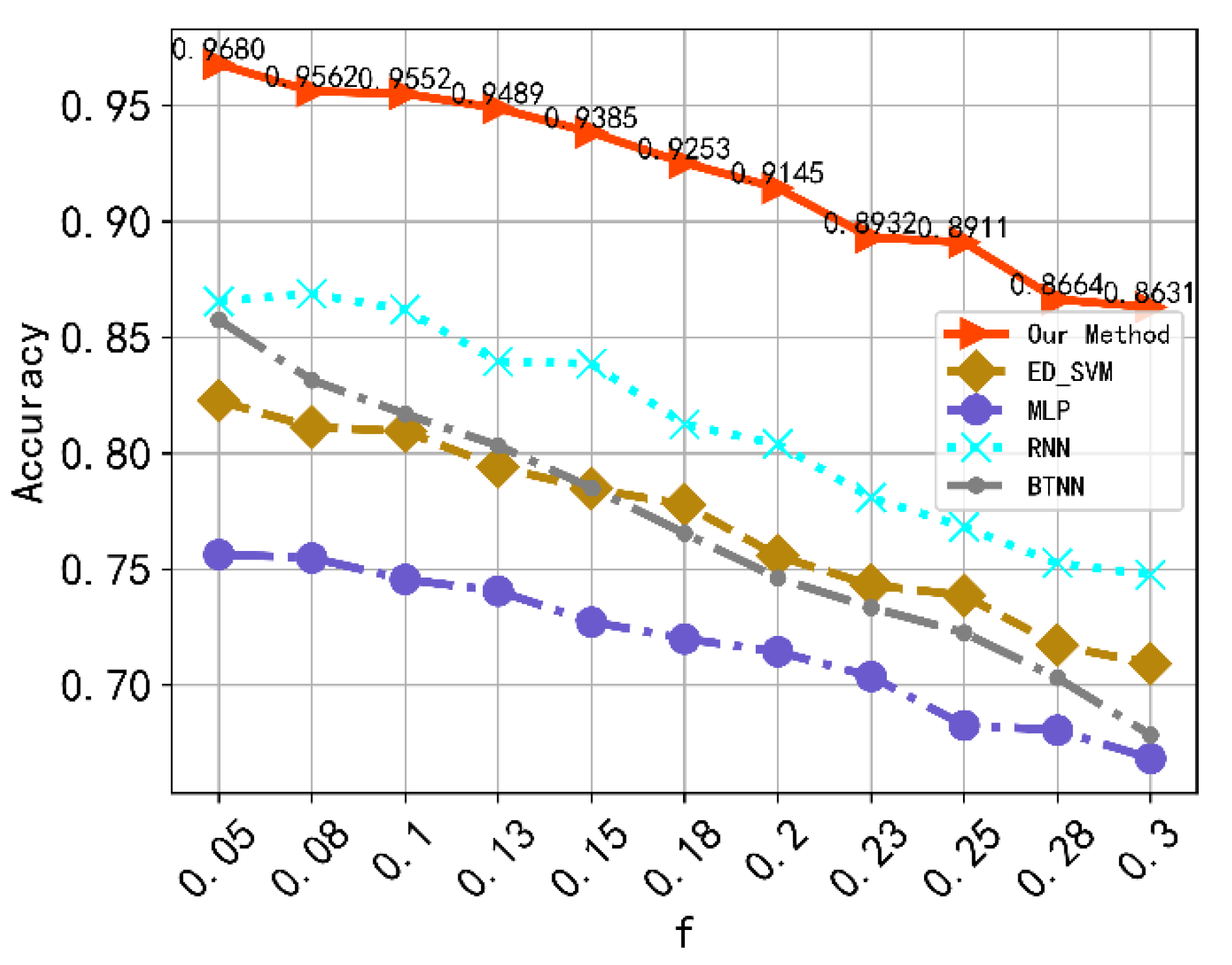
6.2. Contrast Experiments

In this section, the proposed method is compared with the methods in the literature [11,12,34,35]. These methods are reproduced to identify ship targets in the AIS dataset used in this paper. The weighted recall, weighted precision, and weighted F1-score are selected as the evaluation indicators. The recall, precision, and F1-score are indicators used to evaluate binary classification. By assigning weights to their values, multiple classifications can be evaluated. The weight is the proportion of the number of each category. The experimental results in Table 1 show that the recognition ability of the proposed method exceeds that of the existing methods. They identify ship targets only using the trajectory information. The Bayesian transformer neural network (BTNN) method proposed in a study [35] performs well in target recognition. However, when the number of samples in the dataset decreases, the recognition ability of the BTNN decreases, which is a common problem for deep learning. In this study [35], there were 212,508 trajectories in the dataset, while 28,800 were used in this research. By enhancing the trajectory information with the context knowledge, the proposed method outperformed other methods. This further proves the effectiveness of trajectory information enhancement and the effectiveness of the feature fusion network. The method of context enhancement also provides a solution to overcome the problem of deep learning capability degradation caused by the reduction of dataset size. The network model in this paper adopts a transformer and LSTM network to extract trajectory features and context features, respectively, and then the fusion features are identified. The model can make use of the two kinds of information, and the extracted features are more discriminative.
In the real world, noise is everywhere. The trajectory data collected by various sensors also have different levels of noise. To verify the recognition ability of the proposed method under different levels of noise, Gaussian noise is added to the input data in this experiment. More specifically, the noise data are added to the latitude (lat), longitude (lon), speed over ground (sog), course over ground (cog), and timestamp (t) in the trajectory data. The noise data are generated by setting the mean and standard of the matrix. The mean value of the Gaussian noise is 0, and the standard deviation is f  [0.05, 0.08, 0.10, 0.13, 0.15, 0.18, 0.20, 0.23, 0.25, 0.28, 0.30]. Figure 9 shows the curves of the accuracy of the four methods changing with f. With the increase in f, the recognition accuracy of the four methods presents a declining trend. However, the recognition accuracy of our method is always higher than that of other methods under different noise levels. When f increases to 0.30, the recognition accuracy of our method is 0.8631, which maintains a high level. This shows that our method has a strong recognition ability in a noisy environment.

6.3. Validation on Other Maritime Area Datasets

To demonstrate the generality of the proposed method, the method is applied to another maritime area near the east coast of North America. In this area, the intensity of the traffic is lower than that of the area where the previously used data are from. Four main ship types are selected from the AIS data: fishing, pleasure craft, passenger, and cargo ships. Figure 10 shows the grid graph. Figure 11 shows the marks on the coastline. Two groups of experiments are set. The first group of experiments only recognizes the target by trajectory information, and the other group recognizes the target by trajectory and context information. The accuracy of the first group is 79.61%, while that of the other is 87.34%. By enhancing the trajectory with context information, the accuracy is increased by 7.73%. The results indicate that the proposed method is general in different scenarios.

7. Conclusions

In this paper, we propose a method for ship target recognition based on context-enhanced trajectories. By constructing a context knowledge base, the trajectory information can be contextually enhanced to make the trajectory more discriminative. We use the deep learning model to automatically extract the trajectory feature and the context feature. Then, the features are fused to obtain a comprehensive feature. The fused feature is used to recognize the ship targets. Offline training and online recognition are adopted to complete the recognition task. AIS data are used for verification, and the results show that the proposed method has high recognition accuracy and strong anti-noise ability. The context enhancement method can improve the recognition ability.
There are also some limitations in this study. The construction of a context knowledge base is complicated. For example, the number of markers that are selected on the shore is large, and the selection work is somewhat difficult. The uncertainty of marker selection and the approximate calculation of distance to shore lead to the deviation of context information extraction. In addition, the recognition task focuses on one part of the ocean, while the origin or destination port may be outside of the map segment. The context information of distances from target to ports may not be comprehensive. Although the deviation in the context information does not lead to the failure of the recognition task, it limits the improvement of the recognition ability. In future work, more attention should be given to the accuracy of context information construction. In addition, more context information needs to be mined. This research attempts to fuse context information with trajectory information to recognize ship targets. The experimental results show the effectiveness of this operation. Therefore, in future work, richer and deeper context information can be considered for extraction.

Author Contributions

Conceptualization, Wei Xiong and Yaqi Cui; methodology, Zhan Kong; validation, Zhenyu Xiong; data curation, Zhenyu Xiong; writing—original draft preparation, Zhan Kong; writing—review and editing, Wei Xiong; visualization, Pingliang Xu; supervision, Yaqi Cui; project administration, Yaqi Cui; and funding acquisition, Yaqi Cui. All authors have read and agreed to the published version of the manuscript.

Funding

This research was funded by the National Natural Science Foundation of China, Grant Numbers 61790554 and 62001499.

Data Availability Statement

The data are available in Section 5.2.

Conflicts of Interest

The authors declare no conflict of interest.

References

  1. Zou, Y.; Zhao, L.; Qin, S.; Pan, M.; Li, Z. Ship target detection and identification based on SSD_MobilenetV2. In Proceedings of the 2020 IEEE 5th Information Technology and Mechatronics Engineering Conference (ITOEC), Chongqing, China, 12–14 June 2020. [Google Scholar]
  2. Zhang, D.; Zhan, J.; Tan, L.; Gao, Y.; Župan, R. Comparison of two deep learning methods for ship target recognition with optical remotely sensed data. Neural Comput. Appl. 2021, 33, 4639–4649. [Google Scholar] [CrossRef]
  3. Salerno, E. Using Low-Resolution SAR Scattering Features for Ship Classification. IEEE Geosci. Remote Sens. Lett. 2022, 19, 1–4. [Google Scholar] [CrossRef]
  4. Lee, S.J.; Lee, K.J.; Sensing, R. Efficient Generation of Artificial Training DB for Ship Detection Using Satellite SAR Images. IEEE J. Sel. Top. Appl. Earth Obs. Remote Sens. 2021, 14, 11764–11774. [Google Scholar] [CrossRef]
  5. Chuang, L.Z.-H.; Chen, Y.-R.; Chung, Y.-J. Applying an Adaptive Signal Identification Method to Improve Vessel Echo Detection and Tracking for SeaSonde HF Radar. Remote Sens. 2021, 13, 2453. [Google Scholar] [CrossRef]
  6. Chen, J.S.; Dao, D.T.; Chien, H. Ship Echo Identification Based on Norm-Constrained Adaptive Beamforming for an Arrayed High-Frequency Coastal Radar. IEEE Trans. Geosci. Remote Sens. 2020, 59, 1143–1153. [Google Scholar] [CrossRef]
  7. Wang, W.; Xia, F.; Nie, H.; Chen, Z.; Gong, Z.; Kong, X.; Wei, W. Vehicle trajectory clustering based on dynamic representation learning of internet of vehicles. IEEE Trans. Intell. Transp. Syst. 2020, 22, 3567–3576. [Google Scholar] [CrossRef]
  8. Noyes, S.P. Track classification in a naval defence radar using fuzzy logic. In Proceedings of the Target Tracking & Data Fusion, Birmingham, UK, 9 June 1998. [Google Scholar]
  9. Kouemou, G.; Opitz, F. Radar target classification in littoral environment with HMMs combined with a track based classifier. In Proceedings of the International Conference on Radar, Adelaide, SA, Australia, 2–5 September 2008. [Google Scholar]
  10. Ghadaki, H.; Dizaji, R. Target track classification for airport surveillance radar (ASR). In Proceedings of the 2006 IEEE Conference on Radar, Verona, NY, USA, 24–27 April 2006. [Google Scholar]
  11. Bakkegaard, S.; Blixenkrone-Moller, J.; Larsen, J.J.; Jochumsen, L. Target Classification Using Kinematic Data and a Recurrent Neural Network. In Proceedings of the 2018 19th International Radar Symposium (IRS), Bonn, Germany, 20–22 June 2018. [Google Scholar]
  12. Ichimura, S.; Zhao, Q. Route-Based Ship Classification. In Proceedings of the 2019 IEEE 10th International Conference on Awareness Science and Technology (iCAST), Morioka, Japan, 23–25 October 2019. [Google Scholar]
  13. Stenneth, L.; Wolfson, O.; Yu, P.S.; Xu, B. Transportation mode detection using mobile phones and GIS information. In Proceedings of the 19th ACM SIGSPATIAL International Conference on Advances in Geographic Information, Chicago, IL, USA, 1–4 November 2011. [Google Scholar]
  14. Siła-Nowicka, K.; Vandrol, J.; Oshan, T.; Long, J.A.; Demšar, U.; Fotheringham, A.S. Analysis of human mobility patterns from GPS trajectories and contextual information. Int. J. Geogr. Inf. Sci. 2016, 30, 881–906. [Google Scholar] [CrossRef] [Green Version]
  15. Buchin, M.; Dodge, S.; Speckmann, B.J.S. Context-Aware Similarity of Trajectories. In Proceedings of the International Conference on Geographic Information Science, Columbus, OH, USA, 18–21 September 2012. [Google Scholar]
  16. Ahearn, S.C.; Dodge, S.; Simcharoen, A.; Xavier, G.; Smith, J.L. A context-sensitive correlated random walk: A new simulation model for movement. Int. J. Geogr. Inf. Sci. 2017, 31, 867–883. [Google Scholar] [CrossRef]
  17. Bagnall, A.; Lines, J.; Hills, J.; Bostrom, A. Time-series classification with COTE: The collective of transformation-based ensembles. IEEE Trans. Knowl. Data Eng. 2015, 27, 2522–2535. [Google Scholar] [CrossRef]
  18. Lines, J.; Bagnall, A. Time series classification with ensembles of elastic distance measures. Data Min. Knowl. Discov. 2015, 29, 565–592. [Google Scholar] [CrossRef]
  19. Hills, J.; Lines, J.; Baranauskas, E.; Mapp, J.; Bagnall, A. Classification of time series by shapelet transformation. Data Min. Knowl. Discov. 2013, 28, 851–881. [Google Scholar] [CrossRef] [Green Version]
  20. Serrano-Guerrero, J.; Romero, F.P.; Olivas, J.A. Fuzzy logic applied to opinion mining: A review. Knowledge-Based Syst. 2021, 222, 107018. [Google Scholar] [CrossRef]
  21. Reddy, G.T.; Reddy, M.; Lakshmanna, K.; Rajput, D.S.; Kaluri, R.; Srivastava, G. Hybrid genetic algorithm and a fuzzy logic classifier for heart disease diagnosis. Evol. Intell. 2020, 13, 185–196. [Google Scholar] [CrossRef]
  22. Ahn, S.; Couture, S.V.; Cuzzocrea, A.; Dam, K.; Grasso, G.M.; Leung, C.K.; McCormick, K.L.; Wodi, B.H. A fuzzy logic based machine learning tool for supporting big data business analytics in complex artificial intelligence environments. In Proceedings of the 2019 IEEE international conference on fuzzy systems (FUZZ-IEEE), New Orleans, LA, USA, 23–26 June 2019; pp. 1–6. [Google Scholar]
  23. Mohajerin, N.; Histon, J.; Dizaji, R.; Waslander, S.L. Feature extraction and radar track classification for detecting UAVs in civillian airspace. In Proceedings of the 2014 IEEE Radar Conference (RadarCon), Cincinnati, OH, USA, 19–23 May 2014. [Google Scholar]
  24. Espindle, L.P.; Kochenderfer, M. Classification of primary radar tracks using Gaussian mixture models. IET Radar Sonar Navig. 2010, 3, 559–568. [Google Scholar] [CrossRef]
  25. Sheng, K.; Liu, Z.; Zhou, D.; He, A.; Feng, C. Research on Ship Classification Based on Trajectory Features. J. Navig. 2017, 71, 100–116. [Google Scholar] [CrossRef]
  26. Yumu, D.; Sarikaya, T.B.; Efe, M.; Soysal, G.; Kirubarajan, T. Track Based UAV Classification Using Surveillance Radars. In Proceedings of the 2019 22th International Conference on Information Fusion (FUSION), Ottawa, ON, Canada, 2–5 July 2019. [Google Scholar]
  27. Maguire, D.J. An overview and definition of GIS. Princ. Appl. 1991, 1, 9–20. [Google Scholar]
  28. Wang, H.; Liu, Z.; Liu, Z.; Wang, X.; Wang, J. GIS-based analysis on the spatial patterns of global maritime accidents. Ocean. Eng. 2022, 245, 110569. [Google Scholar] [CrossRef]
  29. Zhou, X.; Cheng, L.; Li, M. Assessing and mapping maritime transportation risk based on spatial fuzzy multi-criteria decision making: A case study in the South China sea. Ocean Eng. 2020, 208, 107403. [Google Scholar] [CrossRef]
  30. Lv, Y.; Xiong, W.; Zhang, X.; Cui, Y. Fusion-based correlation learning model for cross-modal remote sensing image retrieval. IEEE Geosci. Remote Sens. Lett. 2021, 19, 1–5. [Google Scholar] [CrossRef]
  31. Lv, Y.; Zhang, X.; Xiong, W.; Cui, Y.; Cai, M. An End-to-End Local-Global-Fusion Feature Extraction Network for Remote Sensing Image Scene Classification. Remote Sens. 2019, 11, 3006. [Google Scholar] [CrossRef] [Green Version]
  32. Vaswani, A.; Shazeer, N.; Parmar, N.; Uszkoreit, J.; Jones, L.; Gomez, A.N.; Kaiser, Ł.; Polosukhin, I. Attention is all you need. In Proceedings of the Advances in Neural Information Processing Systems, Long Beach, CA, USA, 4–9 December 2017; pp. 5998–6008. [Google Scholar]
  33. Hochreiter, S.; Schmidhuber, J. Long short-term memory. Neural Comput. 1997, 9, 1735–1780. [Google Scholar] [CrossRef] [PubMed]
  34. De Vries, G.K.D.; Van Someren, M. Machine learning for vessel trajectories using compression, alignments and domain knowledge. Expert Syst. Appl. 2012, 39, 13426–13439. [Google Scholar] [CrossRef]
  35. Kong, Z.; Cui, Y.; Xiong, W.; Yang, F.; Xiong, Z.; Xu, P. Ship Target Identification via Bayesian-Transformer Neural Network. J. Mar. Sci. Eng. 2022, 10, 577. [Google Scholar] [CrossRef]
Figure 1. Overall process of the proposed method.
Ijgi 11 00584 g001
Figure 2. Thermal maps of active areas for different types of ships. (a) Thermal map over the entire area. (b) Thermal map shown in detail.
Ijgi 11 00584 g002
Figure 3. Network structure.
Ijgi 11 00584 g003
Figure 4. AIS data plot.
Ijgi 11 00584 g004
Figure 5. Grid map of maritime traffic density.
Ijgi 11 00584 g005
Figure 6. Marks on the coastline.
Ijgi 11 00584 g006
Figure 7. Confusion matrices of the results. (a) Confusion matrix without context enhancement. (b) Confusion matrix with context enhancement. (c) Confusion matrix under context information.
Ijgi 11 00584 g007aIjgi 11 00584 g007b
Figure 8. Visualization of local recognition results.
Ijgi 11 00584 g008
Figure 9. Curves of the accuracy of the four methods changing with f.
Ijgi 11 00584 g009
Figure 10. Grid map of maritime traffic density in the maritime area near the east coast of North America.
Ijgi 11 00584 g010
Figure 11. Marks on the coastline in the maritime area near the east coast of North America.
Ijgi 11 00584 g011
Table 1. Results of contrast experiments.
MethodWeighted RecallWeighted PrecisionWeighted F1-Score
SVM [34]0.82950.82860.8244
MLP [12]0.77220.76660.7635
RNN [11]0.88890.88970.8885
BTNN [35]0.90210.90480.9017
Our method0.97140.97140.9713
Publisher’s Note: MDPI stays neutral with regard to jurisdictional claims in published maps and institutional affiliations.

