Article

Research into the Optimal Regulation of the Groundwater Table and Quality in the Southern Plain of Beijing Using Geographic Information Systems Data and Machine Learning Algorithms

1
College of Water Resources and Hydropower Engineering, North China Electric Power University, Beijing 102206, China
2
School of Water Resources and Environment, China University of Geosciences (Beijing), Beijing 100083, China
*
Author to whom correspondence should be addressed.
ISPRS Int. J. Geo-Inf. 2022, 11(10), 501; https://doi.org/10.3390/ijgi11100501
Submission received: 25 August 2022 / Revised: 19 September 2022 / Accepted: 23 September 2022 / Published: 26 September 2022

Abstract

:
The purpose of this paper is to provide new ideas and methods for the sustainable use of groundwater in areas with serious groundwater overexploitation and serious groundwater pollution. Geographic information systems (GIS) were combined with machine learning algorithms, water resources optimization technology, and groundwater numerical simulation to optimize the regulation of the groundwater table and quality beneath the Daxing District in the southern plain of Beijing. By collecting local consumption and supply data and observations of the groundwater table and quality in the connected aquifer beneath Daxing for the years 2006–2020, the corresponding water demands and groundwater impact were extrapolated for the years 2021–2025 based on the basis of the existing development model. Through the combination of GIS and machine learning algorithms, the NO3-N concentration of local groundwater monitoring points in wet years, normal years, and dry years were predicted. With respect to NO3-N pollution, three new groundwater exploitation regimes were devised, which we numbered 1 to 3. The optimal allocation of water resources was then calculated for wet year, typical year, and dry year scenarios for the year 2025. By comparing the water shortage, groundwater utilization rate, and NO3-N pollution under the new groundwater exploitation regimes, the optimal groundwater exploitation mode for the three different types of hydrological year was determined. The results indicate that NO3-N pollution was greatly reduced after the adoption of the optimal regimes and that the groundwater table demonstrated rapid recovery. These results can be of great help in realizing the management, supervision, and regulation of groundwater by combining GIS with machine learning algorithms.

1. Introduction

With the rapid growth of urban populations in recent years, urban water consumption has increased rapidly [1,2]. In northern China, where surface water is limited, urban water supplies are mostly sourced from groundwater. Growing urban water consumption in northern China has led to the over-exploitation of local groundwater resources, and this in turn has led to problems such as a continuous decline of the water table, land subsidence, and deterioration of groundwater quality [3,4]. To address the environmental problems caused by long-term groundwater overexploitation in the north, the Chinese government has launched the South-to-North Water Diversion Project.
Located in the northern part of the North China Plain, the nation’s capital city of Beijing is one of the cities affected by groundwater overexploitation. Since 2014, South-to-North water transfer to Beijing has replaced some groundwater, but groundwater still accounts for 30–40% of Beijing's total water supply. Moreover, a considerable mass of pollutants is discharged into surface water and from there into the groundwater, a fact which magnifies the problem of water supply security [5]. Therefore, how best to realize the sustainable utilization of groundwater resources while ensuring economic and social development has become an urgent problem to be solved.
GIS (Geographic Information Systems) is a technology that is widely used to collect, store, manage, analyze, and express spatial data [6]. GIS spans the intellectual realms of computer science, surveying, cartography, and geography, and has a wide range of applications. Not only does GIS play an important role in environmental resource management and planning, it has become an important tool in other fields such as urban management, engineering construction, commercial decision-making, and strategic analysis for the military, and has therefore become an essential working system for many institutions [7,8,9]. As a part of the global hydrological cycle, groundwater has obvious geographical distribution characteristics. As GIS has powerful geospatial analysis capabilities, it can be combined with machine prediction models, water resource optimization technology, and groundwater numerical simulation to achieve optimal regulation of the groundwater table and quality.
Water quality prediction is a basic function of water supervision and management [10]. At present, water quality prediction methods mainly involve time series prediction [11], gray-box prediction [12], fuzzy logic prediction [13,14], solute transport simulation [15,16], and machine learning algorithms [17,18]. While the time series method has a relatively sound theoretical basis, only the temporal response of the predicted water quality index is considered [19]. Water quality prediction is a very complex problem, and there are many factors affecting the prediction of water quality parameters. The accuracy of prediction in the future is poor only due to changes in the prediction index itself. The gray-box prediction method is easy to operate and suitable for situations where water quality monitoring data is incomplete, but it is easily affected by unstable data, resulting in a large prediction error in such cases [20]. Fuzzy logic prediction can handle uncertainty in the process of water quality prediction, although the calculation effort is large [21]. While the finite difference method can be used to simulate solute transport by flowing groundwater in the aquifer, the boundary conditions are not easy to determine [22,23].
The machine learning algorithm approach has a clear meaning, and adds artificial thinking and judgment along with high precision [24]. At present, machine learning algorithms mainly include neural networks and statistical learning methods. Commonly used neural network algorithms include back-propagation neural networks [25], radial basis function neural networks [26], recurrent neural networks [27], and long short-term memory neural networks (LSTMs) [28,29,30]. Statistical learning methods include decision trees [31,32], random forests (RFs) [33,34], and support vector machines (SVMs) [35,36]. With such a variety of powerful techniques on offer, effective groundwater quality prediction and control can be realized by combining GIS data with machine learning algorithms.
In this paper, Daxing District in the southern plain of Beijing is adopted as a case study. Thiessen polygons were generated around groundwater quality monitoring points. A GIS regional analysis tool was then used to extract the water consumption and economic development of each township. Finally, the groundwater quality in the study area from 2021 to 2025 was predicted using machine learning algorithms. According to the obtained results, the groundwater quality and the water table in the study area can be regulated by optimizing the allocation of water resources and by numerical simulation of the aquifer. The research methods in this paper can provide a theoretical foundation for the sustainable utilization of water resources in areas where groundwater is the main water source.

2. Materials and Methods
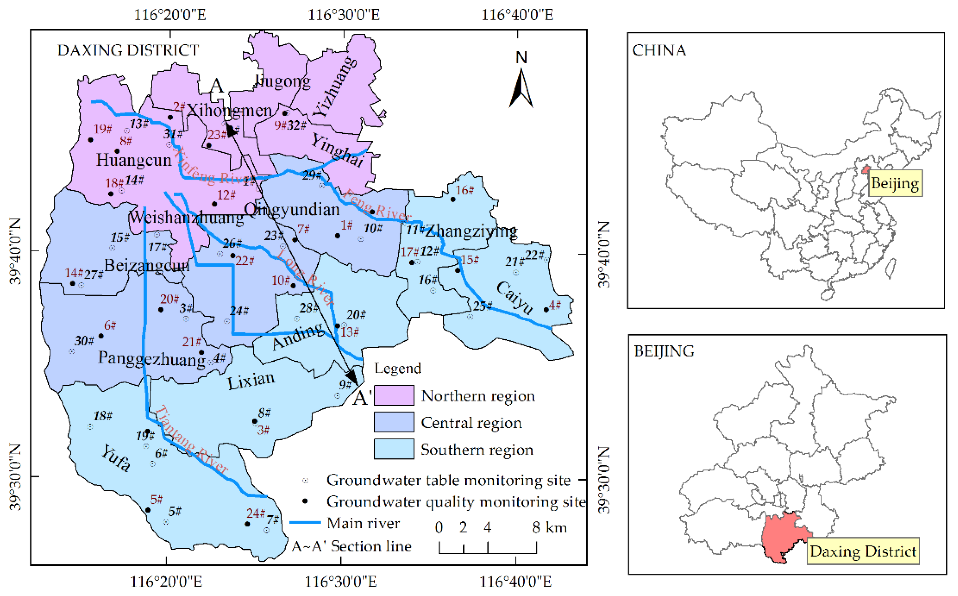
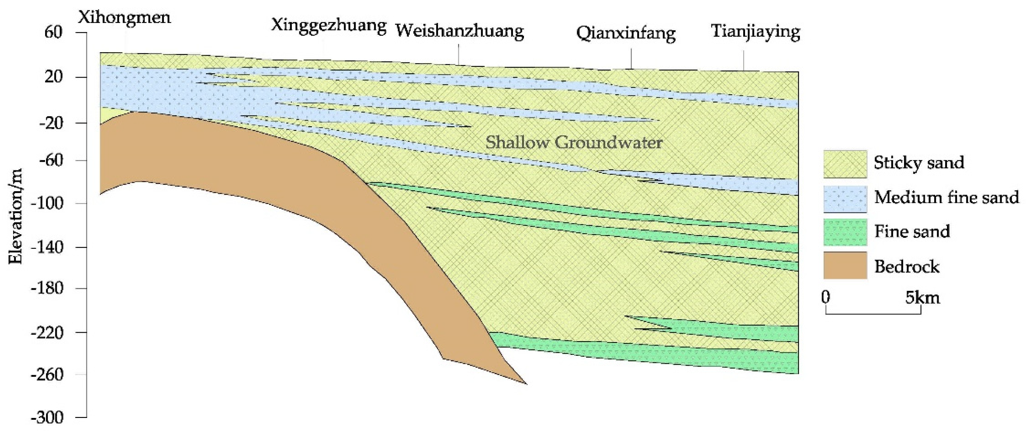
2.1. Study Area

Daxing District is located in the southern plain of Beijing, in a range of map coordinates that spans 116°13′–116°43′ E and 39°26′–39°51′ N. The district is divided into fourteen townships (Figure 1), and the total area of the district is approximately 1036 km2. This part of China has a warm temperate semi-humid continental monsoon climate with four distinct seasons. The average annual rainfall is 510.1 mm; the rainfall is unevenly distributed within the year and varies greatly from year to year. The average annual temperature is 11.7 °C, and the maximum frozen soil depth is 69 cm. The district is on the alluvial–proluvial plain of the Yongding River. Its terrain is flat, with an elevation of 9–73 m (the elevation reference system is the 1956 Yellow Sea Elevation System of China) and a topographic gradient of 0.5–2.0‰. Its soil type is mainly sandy loam, which gradually changes from coarse to fine as one travels from west to east. The thickness of the groundwater aquifer beneath is 80–120 m (Figure 2). The aquifer is mainly composed of medium and fine sand layers of the quaternary loose layer. Because the aquifer is generally permeable, the groundwater table is uniform. There are four main rivers in the study area, namely, the Xinfeng River, the Fenghe River, the Xiaolong River, and the Dalong River. The rivers in the district mainly originate within it; the main source of recharge is atmospheric precipitation. The course of the rivers is shown in Figure 1. Due to the deep groundwater table in the study area, the river and the groundwater table are disconnected. The rivers recharge groundwater mainly through seepage, forming a river with a suspended saturation zone under the riverbed, an unsaturated zone, and a groundwater aquifer system (Figure 3). From 2006 to 2020, the average total recharge of groundwater was 2.29 × 10⁸ m3, and the total discharge of groundwater was 2.21 × 10⁸ m3. It can be seen that the total recharge of groundwater was slightly larger than the total discharge. However, because the recharging of well irrigation depends on the groundwater generated after the seepage of farmland irrigation water, it should not be included in the total amount of groundwater resources. Therefore, the amount of groundwater water resources should be the total recharge amount minus the return recharge from well irrigation, meaning that the average groundwater resource amount from 2006 to 2020 was 2.00 × 10⁸ m3. It can be seen that the groundwater discharge amount from 2006 to 2020 was greater than the groundwater resource amount.

2.2. Data Sources

2.2.1. Groundwater Table and Quality Data

The groundwater table data were mainly derived from a long-term monthly monitoring data series generated by 32 observation wells from 2006 to 2020. The locations of the monitoring wells are shown in Figure 1. The groundwater quality data were mainly derived from the annual monitoring data of 25 shallow groundwater monitoring wells from 2006 to 2020. The locations of these monitoring wells are shown in Figure 1 as well. NO3-N pollution is the main pollutant of groundwater in Beijing, affecting 5% of the total area of the plain. NO3-N pollution has the potential to cause great harm to the health of both humans and livestock [37], and is greatly affected by human activities. Therefore, NO3-N was selected as the evaluation index.

2.2.2. Statistical Data

The statistical data used in this paper were mainly obtained from the following publications, of which the originals are all in Chinese: the water statistical yearbook of Beijing from 2006 to 2020; the statistical yearbook of Daxing District from 2005 to 2020; the data compilation of the third agricultural census of Daxing District in 2016; the second national pollution source census bulletin of Beijing (2017); the regional statistical yearbook of Beijing from 2012 to 2020; the 2020 environmental statistical yearbook of China; the 2018 comprehensive water resources plan of the Daxing District; the 2017 water supply plan for the Xinfeng River Basin of the Daxing District; and the 2019 main data bulletin of the third national land survey of the Daxing District.

2.3. Research Method

2.3.1. Forecast of Water Demand

According to the Beijing 14th Five-Year Plan for Water-saving Society Construction and related research materials [38,39,40], we determined the domestic water demand, industrial water demand, agricultural water demand, and ecological water demand in the study area from 2021 to 2025. The specific calculation process was as follows:
  • Forecast of domestic water demand
Daxing District’s domestic water demand from 2021 to 2025 was calculated from the per capita water consumption and the population using the following formula:
R 1 = S ( 1 + α ) t G ( 1 + β ) t 365 / 1000
In Equation (1), R1 is Daxing’s domestic water consumption in units of 104 m3; S is the current water consumption in L/d∙per person; the current water consumption is based on the actual water consumption in 2020, which was 129.73 L/d∙per person; α is the annual growth rate of water use per person, which is currently 2%; G is the current population in units of 104 persons; the current population is 1.994 × 10⁶ person; and β is the annual growth rate of the population, currently 4%; t is elapsed time in years.
  • Forecast of industrial water demand
Daxing District’s industrial water consumption from 2021 to 2025 was calculated from the water consumption required to generate CNY 10,000 worth of industrial output and the total industrial output using the following formula:
R 2 = g 0 ( 1 + v ) t M 0 ( 1 + v ' ) t
In Equation (2), R2 is Daxing’s industrial water consumption in units of 104 m3; g0 is the current water consumption required to yield CNY 10,000 worth of industrial output in m3/(104 CNY); M0 is the total industrial output value in units of 108 CNY; v represents the annual growth rate of water consumption per 104 CNY of industrial output, currently at −5%; and the annual growth rate of industrial development v’ is 6%.
  • Forecast of agricultural water demand
The rate of water consumption for animal husbandry and aquaculture in Daxing District is very small. The district’s agricultural water demand is used for the irrigation of crops, mainly wheat. Therefore, only the water used for crop irrigation is incorporated into our calculations, as a proxy for total agricultural water demand in Daxing.
R 3 = 1 η ω A
In Equation (3), R3 is Daxing’s agricultural water consumption in units of 104 m3. The symbol η denotes the effective utilization coefficient of irrigation water, meaning the degree of efficiency with which this water is used. The effective utilization coefficient of irrigation water increases by 0.01 every year and is thus expected to be 0.75 in 2025. The symbol ω denotes the annual irrigation water quota, which locally amounts to 2850 m3/hm2 in a wet year and 3300 m3/hm2 in a dry year. A denotes the irrigated area in hm2. According to the main data bulletin of the third national land survey for Daxing (2019), the area of agricultural land in the study area is 26,371.65 hm2; thus, we have assigned this value to A.
  • Forecast of ecological water demand
From 2006 to 2020, the consumption of water in Daxing for ecological purposes has grown continuously. For the purposes of this paper, the district’s demand for ecological water is forecast on the basis of an annual increase of 1%.
R 4 = e 0 ( 1 + γ ) t
In Equation (4): R4 represents the forecast ecological water demand in units of 104 m3, e0 represents the year-2020 demand of 1.43 × 10⁸ m3, γ represents the annual growth rate (1%), and t represents the elapsed time since 2020 in years.

2.3.2. Machine Learning Algorithms

In this paper, three machine learning algorithms, namely, long short-term memory (LSTM), RF, and support vector regression (SVR), were selected to predict the change of NO3-N concentration in Daxing groundwater from 2021 to 2025. By comparing the accuracy of the prediction models during a validation period, the best prediction model was selected.
The long short-term memory neural network (LSTM) method was first proposed by Hochreiter in 1997 [41]. This algorithm is an improved version of the recurrent neural network (RNN), and is intended to solve the problems of gradient disappearance and gradient explosion caused by the single structure of backpropagation when RNN training a model based on RNN [41]. On the RNN foundation, LSTM erects an input gate, an output gate, a forgetting gate, and a memory unit. These additional gating mechanisms help to overcome gradient problems [42].
The governing equations of the LSTM model are as follows:
Input gate:
i t = σ ( W y i + W i m m t 1 + W t c c t 1 + b i )
Output gate:
f t = σ ( W y f y t + W f m m t 1 + W f c c t 1 + b f )
Neuron activation function:
c t = f t c t 1 + i t tan h ( W c y y t + W c m m t 1 + b c )
Forgetting gate:
o t = σ ( W y o + W o m m t 1 + W o c c t 1 + b 0 )
Memory cell state input:
m t = o t tan h ( c t )
Model output:
Z t = W 2 m m t + b z
In these equations, key terms are defined as follows: y t ( t = 1 , 2 , , T ) is the model input sequence; i t , o t , and f t represent the output values of the input gate, forgetting gate, and output gate at time t, respectively; c t and m t represent the activation state of the neuron and memory cell state inputs at time t, respectively; W is the weighting coefficient matrix between different layers; σ is the sigmoid activation function; tanh is the hyperbolic tangent activation function; and Z t ( t = 1 , 2 , , T ) is the model output sequence.
RF is a statistical learning method proposed by Breiman in 2001 on the foundation of the Bagging algorithm [43]. The algorithm mainly consists of a sub-training sample set and a sub-decision tree model. The sub-training sample set uses the bootstrap resampling method to extract multiple sub-training sample sets with the same sample size as the original sample from the original sample, then constructs a sub-decision tree model for each sub-training sample set. In this way, the RF model is generated. Each sub-decision tree model generates a prediction, and the final prediction is obtained by voting. Because the algorithm has good tolerance for outliers and noise and is not prone to overfitting, it shows high simulation accuracy across many different theories and examples [44,45].
SVM is a machine learning algorithm proposed by Vapnik in 1995 [46]. It is a supervised learning model based on statistical learning theory and is mainly used to solve classification and regression problems. The basic idea of SVM is to use a kernel function to convert low-dimensional nonlinear problems into high-dimensional linear problems and then to use linear methods to solve the original nonlinear problems in high-dimensional feature space. Because SVM has the advantages of simple structure and theoretical global optimality, it is the best of the three methods at addressing problems such as small samples, nonlinearity, and high dimensionality.

2.3.3. Optimal Allocation Model for Water Resources

  • Objective function
The degree of water scarcity has an important impact on social stability, while the cost of water determines the economic benefits of water use. The objective function that we have chosen aims, as far as possible, to minimize total water shortage and total water cost at the same time.
(1) Minimum total water shortage
f 1 ( q ) = min j = 1 4 [ R j i = 1 4 q i j ]
In Equation (11), the terms are defined as follows. The function f1(q) is the total water shortage in units of 104 m3; the parameter qij is the annual water supply of the ith water source to the jth type of water user, in units of 104 m3; Rj is the annual water demand of the jth type of users, in units of 104 m3; the parameter i represents the ith water source, whereby i = 1, 2, 3, 4 are numbers that respectively denote surface water, groundwater, reclaimed water, and transferred water; and the parameter j represents the jth water user, whereby j = 1, 2, 3, 4 are numbers that respectively denote domestic water, industrial water, agricultural water, and ecological water.
(2) Minimum water cost
f 2 ( q ) = min i = 1 4 ( j = 1 4 q i j p i )
In Equation (12), the terms not already defined above are defined as follows: the function f2(q) is the cost of water in units of 104 CNY; pi is the unit price of water supply for the ith water source, in CNY/m3; and the unit price of water supply for each water source is determined according to the existing unit price of water supply in Beijing, which is 0.48 CNY/m3 for surface water, 5.00 CNY/m3 for groundwater, 1.00 CNY/m3 for reclaimed water, and 7.44 CNY/m3 for transferred water.
  • Constraint condition
(1) Water supply capacity constraints
i = 1 4 j = 1 4 q i j Q z
j = 1 4 q i j Q i
In Equations (13) and (14), Qz is the total available annual volume of all the water sources in units of 104 m3, while Qi is the available annual volume of each water source in units of 104 m3. According to the comprehensive plan for of water resources in Daxing, the maximum available volume of surface water in the study area Q1 is 1572 × 104 m3 in a normal year or a wet year and 1001 × 104 m3 in a dry year. The maximum usable water amount of groundwater Q2 is determined in accordance with whether the year is wet, dry, or normal. The maximum usable volume of groundwater in a wet year is 22,450.66 × 104 m3, the maximum usable volume of groundwater in a normal year is 18,086.54 × 104 m3, and the maximum usable volume of groundwater in a dry year is 14,931.44 × 104 m3. The maximum available volume of transfer water Q3 is 2600.00 × 104 m3. According to the water supply plan for the Xinfeng River Basin of Daxing District, the maximum usable volume of reclaimed water Q4 is 15,987.00 × 104 m3.
(2) water consumption constraints
The four different water uses need to fall between their respective maximum and minimum water demand constraints, as follows:
Q min , j Q j Q max , j
In Equation (15), Qmin,j and Qmax,j represent the minimum water demand and maximum water demand of the jth water user Qj, respectively; the minimum water demands Qmin,1, Qmin,2 for domestic water and industrial water are in each case 99% of the respective nominal water demand, and the maximum demands Qmax,1 and Qmax,2 are each 110% of the respective nominal water demand; the minimum water demands Qmin,3 and Qmin,4 for agricultural water and ecological water are respectively 75% and 70% of each nominal water demand; and the maximum values Qmax,3 and Qmin,4 are each 110% of the respective nominal water demand.
In addition, the water supply and water demand in the above formula should meet non-negativity constraints.
  • Model solution
The water resource optimization model constructed in this paper is a multi-objective optimization problem with constraints. For a solution algorithm, we have chosen the Non-dominated Sorting Genetic Algorithm-II (NSGA-II), which shows good performance in dealing with constrained multi-objective optimization problems [47].
NSGA-II was proposed by Deb in 2002 as an improved version of NSGA. Because NSGA-II adopts the strategy of fast non-dominated sorting and crowding distance, the calculation speed and effect of this algorithm are greatly improved in comparison to NSGA [48].

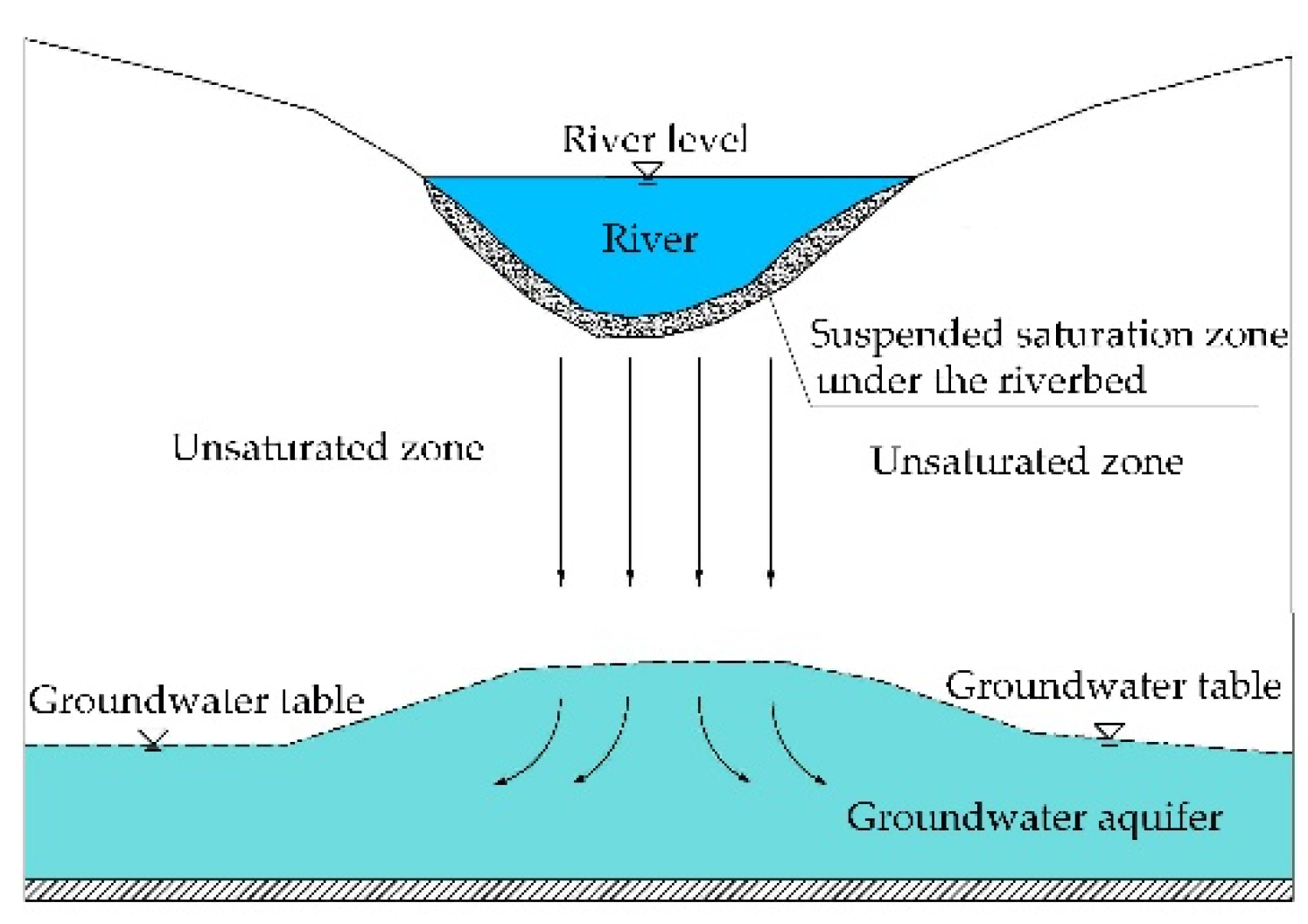
2.3.4. Numerical Simulation of Groundwater Flow

We made use of known drilling and hydrological data for Daxing to establish a hydrogeological model of a conceptual nature. A numerical simulation package called GMS (Groundwater Modeling System 7.1) was used to generalize the aquifer into a two-dimensional non-steady-flow phreatic aquifer with heterogeneity and isotropy. Although parts of this aquifer contain micro-confined water, the medium-fine sand layer in the quaternary loose layer is the main water-bearing medium; permeability extends between the vertically stable water-retaining layers. Thus, the aquifer has the same groundwater table throughout, yielding a thickness in the range of 80–120 m.
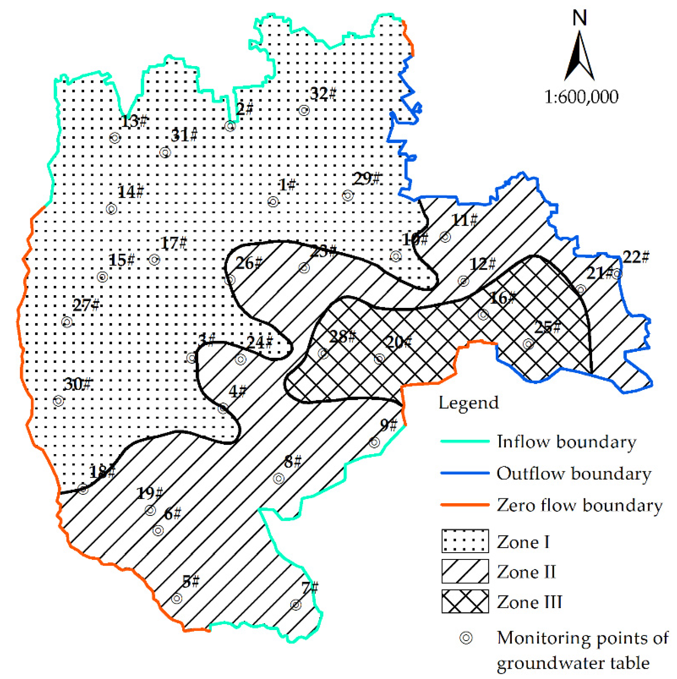
  • Zoning generalization of hydrogeological parameters
In accordance with the drilling data, Daxing was divided into three hydrogeological parameter divisions; this division is shown in Figure 4. The parameters used in the calculation of the water flow model were the permeability coefficient K and the specific yield μ, with their respective value ranges shown in Table 1.
  • Boundary condition generalization
The direction of groundwater flow in Daxing is generally from west to east. In accordance with the contour distribution of the groundwater table in the Beijing plain and the study area (see Figure 5), the boundaries of the aquifer beneath Daxing were divided into two categories: a constant-flux boundary and a zero-flux boundary. As shown in Figure 4 and Figure 5, the groundwater table contours in the north, northwest, and southwest are parallel to the boundary in ways that create lateral inflow boundaries, while the eastern boundary was a lateral outflow boundary. The groundwater table contours in parts of the west and southeast are perpendicular to zero-flux boundaries. The upper boundary of the aquifer beneath Daxing mainly receives atmospheric precipitation, river supply, and farmland irrigation supply, and is the diving boundary. As average depth of groundwater below the surface of the soil was 17.31 m, evaporation could be ignored. According to the drilling data, most of the aquifer exists above a depth of 120 m, and there is a thicker clay layer beneath it.
  • Mathematical model establishment
In accordance with the conceptual model that has just been described, the groundwater flow beneath Daxing can be generalized into a non-homogeneous and isotropic unsteady flow model for the purposes of more detailed numerical analysis. The mathematical model for simulating the aquifer is as follows:
x [ K ( H B ) H x ] + y [ K ( H B ) H y ] + Q r Q d = μ H t
H ( x , y , t ) | t = 0 = h 0 ( x , y , t )             ( x , y ) D
H ( x , y , t ) | Γ 1 = h 1 ( x , y , t )             ( x , y ) D , t > 0
K ( H B ) H n | Γ 2 = q ( x , y , t )             ( x , y ) D , t > 0
In Equations (16)–(19), the new parameters are as follows: K denotes the permeability coefficient of the aquifer in m/d; H denotes the groundwater table in m; B denotes the aquifer floor elevation in m; Qr denotes the groundwater recharge rate in m3/d; Qd denotes the groundwater discharge rate in m3/d; the parameter μ denotes the specific yield of the aquifer; the parameter h1 is the groundwater table of the boundary point of class I in m; the parameter q denotes the single-width flow rate of the class II boundary in m3/(d∙m); the parameters x and y are coordinates specified in m; D is the calculation area range; the parameter n is the inner normal on the boundary; and the identifiers Γ1 and Γ2 denote class I and II boundaries, respectively.
Equation (16) is the partial differential equation of unsteady flow in the diving plane, which describes the movement of shallow groundwater.
Equations (17)–(19) are the definite solution conditions of Equation (16), for which (17) is the initial condition and (18) and (19) are the boundary conditions.
  • Mathematical model solution
The aquifer beneath Daxing was discretized in accordance with our hydrogeological conceptual model in a manner that took realistic account of the likely levels of simulation accuracy and data accuracy. Spatially, Daxing was divided into a rectangular horizontal grid with a grid spacing of 500 m × 500 m; 4700 such grid blocks were generated. The parameter identification period was set from January 2015 to December 2019, and the stress period was one month, which was divided into sixty stress periods. The verification period was from January 2020 to December 2020, and the stress period was one month, which was divided into twelve stress periods. The water flow simulation data for the aquifer were input into the Modflow module in GMS (Groundwater Modeling System 7.1) to evaluate the changes in the groundwater flow field.
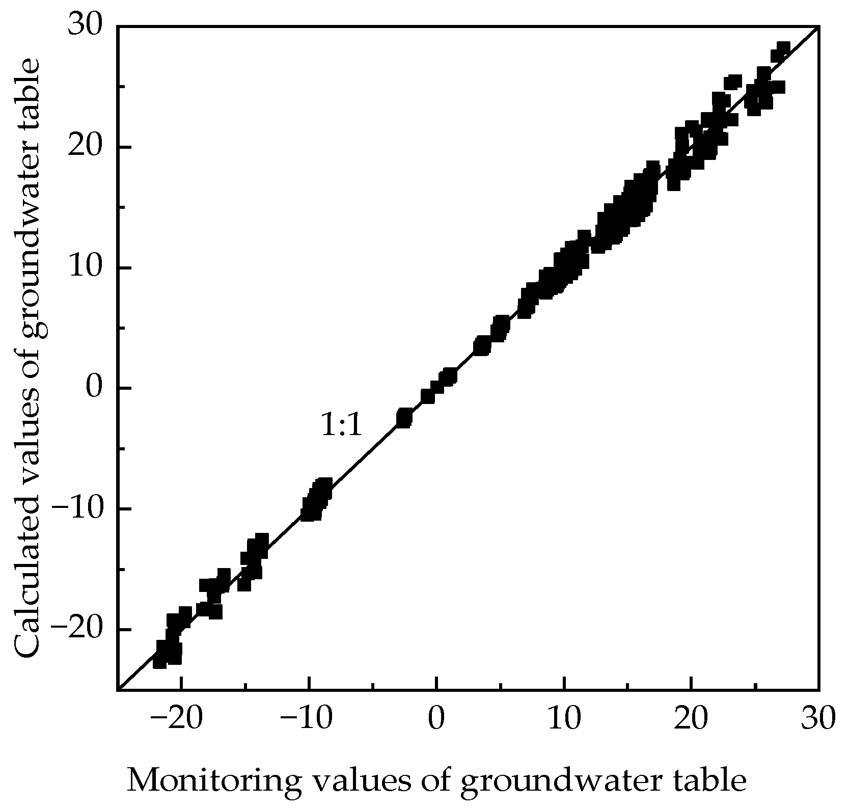
  • Model identification and validation
We used the measured data from 32 groundwater level monitoring points from January 2015 to December 2019 to identify groundwater levels, and used the groundwater table data from the same 32 monitoring points from January 2020 to December 2020 to verify the model.
  • Processing of Source and Sink Items
The groundwater recharge sources in Daxing principally comprised the atmospheric precipitation infiltration recharge, river infiltration recharge, well irrigation return recharge, and groundwater lateral inflow.
The principal discharges comprised artificial exploitation (including industrial water, domestic water, agricultural water, and ecological water) and ground water lateral outflow. The source and sink items from 2015 to 2020 were obtained through the groundwater balance calculation. The results of these calculations are shown in Table 2.
2.
Model Identification and Verification
The initial flow field for model simulation was that of 1 January 2015. The groundwater flow model was identified and validated using data from the 32 groundwater table monitoring wells from January 2015 to December 2019 and from January 2020 to December 2020, respectively. By changing the model parameters, adjusting the boundary conditions, and repeating the trial calculations, the errors between the calculated and observed values at most of the observation wells could be brought within the simulation accuracy requirements. In the process of groundwater flow simulation and identification, the boundary conditions and model parameters, such as specific yield μ and permeability coefficient k, were substantially adjusted. The ratio between the calculated level and the actual level of the groundwater table during the validation period of the groundwater flow model is shown in Figure 6. It can be seen from Figure 6 that the ratio of the calculated level to the observed level during the model verification period was around 1:1. The absolute error between the calculated level and the actual level was less than 1 m for 80.50% of the observations, the maximum absolute error was 1.90 m, and the maximum relative error was 13.16%. It can be seen that the overall degree of fit between the calculated groundwater table and the measured groundwater table is good, which meant that the model was able to accurately reflect the actual characteristics of the groundwater flow field under Daxing. Therefore, the model can be used to predict future changes in the groundwater flow field. The identified hydrogeological parameters are shown in Table 3.

3. Results and Discussion

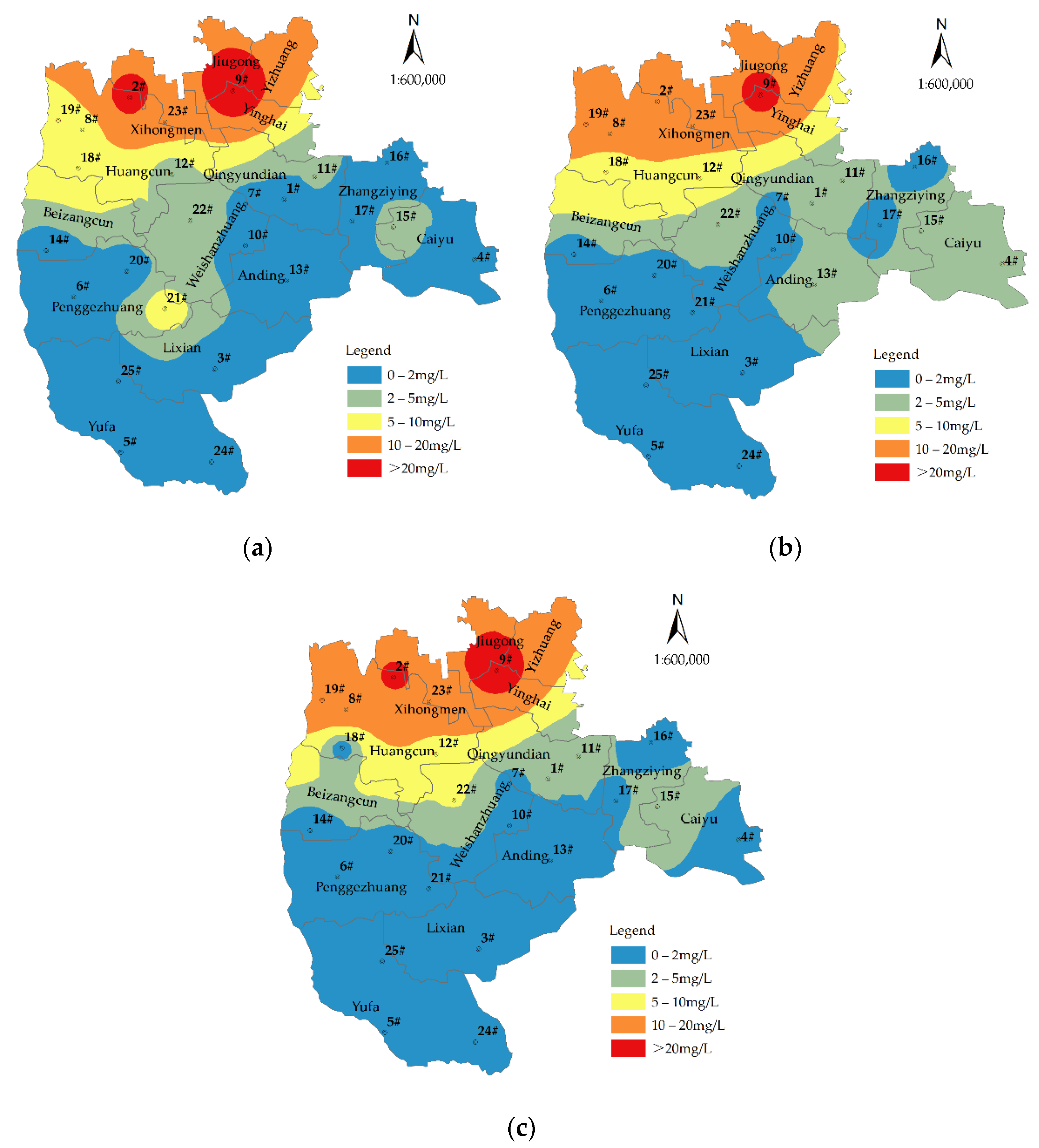
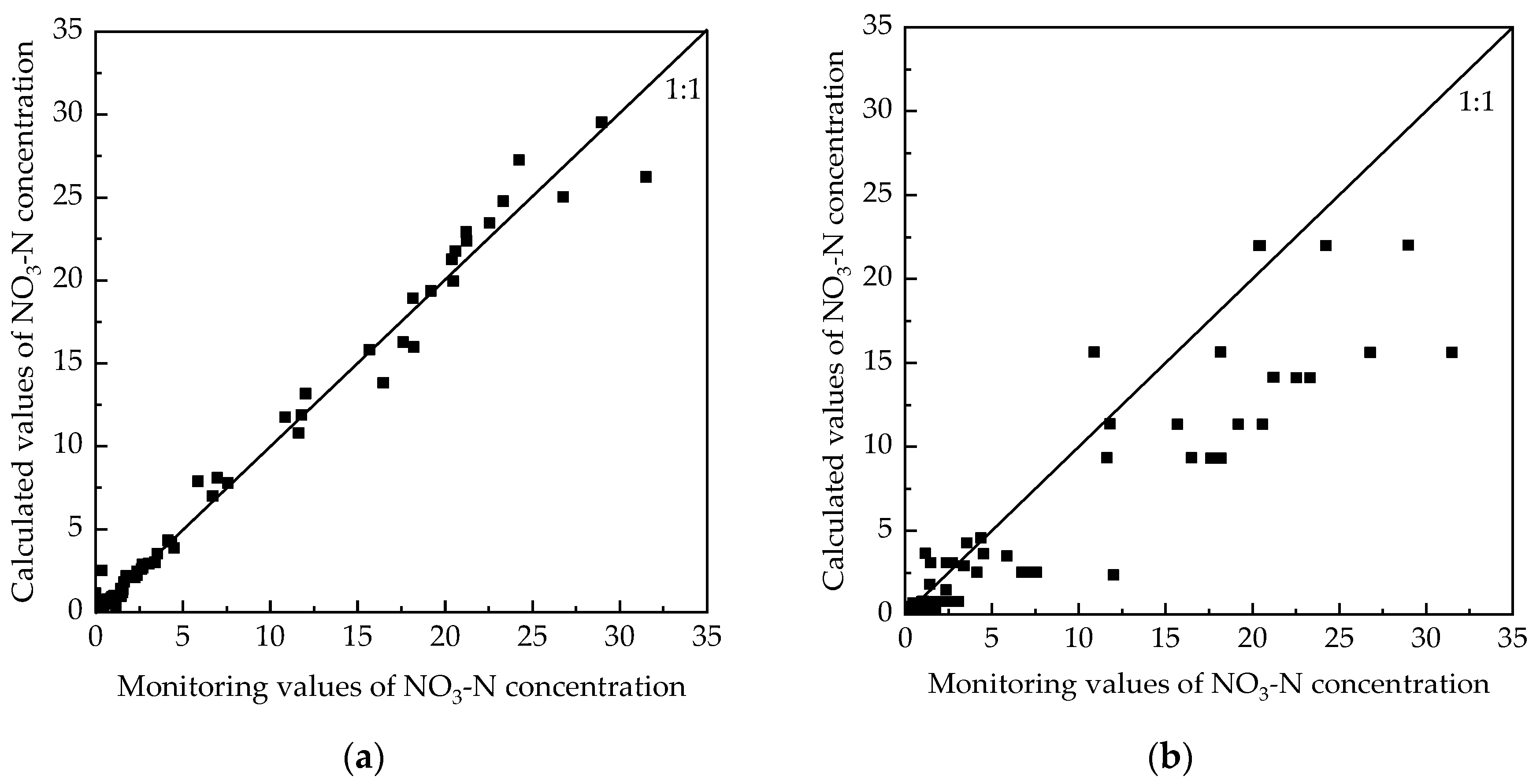
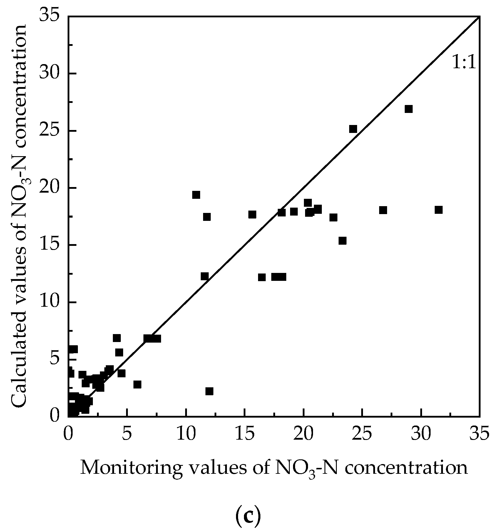
3.1. Forecast of NO3-N Concentration

In accordance with NO3-N monitoring data from the 25 groundwater quality monitoring points from 2006 to 2020, the water quality value of the study area was obtained by interpolation based on the inverse distance weighting method. The maximum number of prediction points within the search radius was 15, and the minimum number of prediction points within the search radius was 10. Through cross-validation, the average error and root mean square error of the NO3-N concentration were found to be 0.09 and 0.53, respectively. These were both small enough to ensure that the average error and root mean square error met the requirements of our evaluation.
To reduce the influence of fluctuations in NO3-N pollution concentration in individual years, the period 2006–2020 was divided into three shorter time periods, namely, 2006–2010, 2011–2015, and 2016–2020. These three time periods correspond to the three five-year plans formulated by the Chinese government, namely, the Eleventh Five-Year Plan for National Economic and Social Development of the People’s Republic of China (2006–2010), the Twelfth Five-Year Plan for National Economic and Social Development of the People’s Republic of China (2011–2015), and the Thirteenth Five-Year Plan for National Economic and Social Development of the People’s Republic of China (2016–2020). Using the grid calculator in our GIS package, the average value of the GIS interpolation results in each time period was generated, yielding final calculation results shown in Figure 7.
It can be seen in Figure 7 that the NO3-N concentration showed an overall increasing trend from 2006 to 2020. Across the whole district, the average concentration of NO3-N from 2006 to 2010 was 5.52 mg/L. On the same basis, the average concentration of NO3-N from 2011 to 2015 was 5.47 mg/L, a slight decrease. However, the average concentration of NO3-N from 2016 to 2020 was 5.92 mg/L, an increase of 0.40 mg/L compared with the average concentration of NO3-N from 2006 to 2010. Overall, these changes indicated that with the continuous increase of urbanization in the study area, NO3-N shows an increasing trend as well.
From a spatial perspective (Figure 7), the average concentration of NO3-N in the northern region of Daxing was greater than that in the central and southern regions. The average concentration of NO3-N in the northern region increased from 12.62 mg/L in 2006–2010 to 14.05 mg/L in 2016–2020. The average concentrations of NO3-N in the central and southern regions remained at 2.67–2.80 mg/L and 1.03–1.57 mg/L from 2006 to 2020, respectively, indicating that the groundwater quality in the central and southern regions was better than that in the northern regions. This might be related to the higher degree of urbanization in the northern regions than in the central and southern regions. According to the 2020 statistical yearbook for Daxing, the industrial output value, tertiary industry output value, and resident population of the northern region accounted for 73.27%, 72.24%, and 60.84% of the equivalents for the whole district, respectively, showing that the NO3-N pollution was largely caused by the intensity of human activity.
We have modeled the current types of water use in Daxing as domestic water, industrial water, agricultural water, and ecological water. Because the current water supply in the study area relies on groundwater as the single most important of the four sources we modeled, it was necessary to evaluate the utility of local groundwater in view of the observed NO3-N pollutant loads.
The water quality standards for domestic water, industrial water, agricultural water, and ecological water are referred to in the relevant official water quality standard for urban water supply (CJ/T 206-2005), the drinking water hygiene standard (GB 5749-2006), the reuse of urban recycling water—water quality standard for industrial uses (GB 19923-2005), the standard for irrigation water quality (GB 5084-2021), and the reuse of urban recycling water—water quality standard for scenic environmental use (GB/T 18921-2019), respectively. Because only the domestic water standards prescribe limits for NO3-N concentration, while the water quality standards for industrial water, agricultural water, and ecological water do not, the groundwater was considered to meet the requirements for industrial water, agricultural water, and ecological water. However, at the same time it was necessary to further evaluate the utility of the local groundwater for domestic water supply in view of its NO3-N concentrations.
To further evaluate the utility of Daxing’s groundwater for domestic water usage, the evaluation had to be carried out in a manner informed by the current water quality standard for urban water supply (CJ/T 206-2005) and the drinking water hygiene standard (GB 5749-2006). According to the drinking water hygiene standard (GB 5749-2006), the limit of NO3-N for groundwater sources is 20 mg/L. However, according to the water quality standard for urban water supply (CJ/T 206-2005), the limit for NO3-N is 10 mg/L (20 mg/L in special cases). Therefore, in cases where there is sufficient water, NO3-N concentrations in the range of 10–20 mg/L mean that water should not be used as domestic water; under conditions of serious water shortage, the NO3-N concentrations in the 10–20 mg/L range are acceptable for domestic water use; and water with an NO3-N concentration above 20 mg/L should not be used as domestic water.
It can be seen from the above analysis that the groundwater in the northern region was seriously polluted and not suitable for domestic water, while the groundwater quality in the central and southern regions was better and could be used as domestic water.
To further predict the NO3-N pollution in wet years, normal years, and dry years from 2021 to 2025, we created Thiessen polygons in ArcGIS around the water quality monitoring points [49,50]; these polygons are shown in Figure 8. Then, using the regional analysis tool in ArcGIS, the Thiessen polygons were used to extract the values of the following eight parameters in each polygon: industrial water use, domestic water use, agricultural water use, industrial output, population, tertiary industry output, agricultural output, and rainfall. Machine learning algorithms were used to predict the changes of NO3-N concentration in wet years, normal years, and dry years from 2021 to 2025.
The three machine algorithms introduced above, namely, LSTM, RF, and SVR, were used to predict the NO3-N concentration change from 2021 to 2025. By comparing the accuracy of their predictions during a validation period, the best prediction model was selected.
The NO3-N concentration of each water quality monitoring point from 2006 to 2016 was used as the training period sample for the three machine learning algorithms, and the NO3-N concentration of each water quality monitoring point from 2017 to 2020 was used as the validation period sample for the three machine algorithms. The mean absolute error, root mean square error, correlation coefficient, and Nash efficiency coefficient were selected as the evaluation accuracy indicators for the machine algorithms. The ratios of the NO3-N concentration calculation values to the monitored values for the three machine algorithms during the validation period are shown in Figure 9. The mean absolute error, root mean square error, correlation coefficient, and Nash efficiency coefficient between the NO3-N concentration calculated value and the monitoring value of the three machine algorithms during the validation period are shown as numbers in Table S1.
It can be seen from Figure 9 that among the three machine algorithms, LSTM has the highest accuracy; for this algorithm, the ratio of the calculated value of NO3-N concentration to the monitored value was always near the 1:1 line. On the other hand, the NO3-N concentration value calculated by the RF and SVR algorithms showed a large deviation from the monitored value, with the deviation of the RF algorithm being the greatest. Table S1 shows that the average absolute error and root mean square error of NO3-N concentration calculated by LSTM were 0.05 and 0.91, figures which were respectively less than both average absolute errors (1.45 and 0.09) and both root mean square errors (3.59 and 2.98) of the NO3-N concentration as calculated by RF and SVR. At the same time, the correlation coefficient and Nash efficiency coefficient between the NO3-N concentration and the actual value calculated by LSTM were 0.98 and 0.98, which were respectively higher than both correlation coefficients (0.93, 0.94) and both Nash efficiency coefficient (0.62, 0.80) as calculated by RF and SVR.
These results, presented in Figure 9 and Table S1 show that the prediction accuracy of LSTM for NO3-N concentration in Daxing was unambiguously better than that of RF and SVR. The order of computational accuracy of the three machine learning algorithms was LSTM > SVR > RF.
Therefore, we chose LSTM as the machine learning system with which to predict the changes of NO3-N concentration in Daxing in wet years, normal years, and dry years from 2021 to 2025.
The water demands for a wet year, a normal year, and a dry year in the years 2021–2025 were calculated in accordance with Equations (1)–(4). The rate of economic development was extrapolated from the average rate of economic development between 2006 and 2020. According to the rainfall sequence from 1956 to 2020, the average rainfall in wet year, normal year, and dry year was 598.40 mm, 482.10 mm and 398.00 mm, respectively. In wet, normal, and dry years, the precipitation guarantee rates were 25%, 50%, and 75%, respectively.
Using the trained LSTM model, the changes in the concentration of NO3-N in a wet year, a normal year, and a dry year from 2021 to 2025 were predicted. The results of this prediction are shown in Figure 10.
As compared with the years 2016 to 2020, average district-wide NO3-N concentrations increased from 5.92 mg/L to 6.34 mg/L, 6.61 mg/L, and 6.96 mg/L in a wet year, a normal year, and a dry year, respectively. In more detail, the NO3-N concentration in the northern region of Daxing increased from 14.05 mg/L to 14.87 mg/L, 15.64 mg/L, and 16.54 mg/L, respectively as the model moved from the period 2016–2020 to the period 2021–2025 (wet year), 2021–2025 (normal year), and 2021–2025 (dry year). It can be seen that the NO3-N concentration in the normal year and the dry year increased more sharply than in the wet year. This can be explained by the fact that groundwater recharge is larger in the wet year than in normal and dry years, thus diluting NO3-N pollution more effectively and transporting the NO3-N out of the Daxing aquifer more rapidly.
To ensure the most socially effective use of water, these figures may be used to create a flexible regime of controls on groundwater use in which the extraction of groundwater for domestic consumption is reduced or prohibited in areas with serious groundwater pollution in ways that take recent rates of dilution and recharge due to rainfall into account.

3.2. Optimal Allocation of Water Resources

To reduce the impact of groundwater NO3-N pollution on domestic water supplies, three groundwater exploitation regimes were established.
Groundwater exploitation regime 1: no area with a groundwater NO3-N concentration above 20 mg/L is to be permitted to contribute its groundwater to the domestic water supply.
Groundwater exploitation regime 2: groundwater extracted from areas with NO3-N concentrations above 10 mg/L but below 20 mg/L are not to be used for domestic purposes, and groundwater extraction from areas with NO3-N concentrations above 20 mg/L are prohibited altogether.
Groundwater exploitation regime 3: groundwater extraction from all areas with an NO3-N concentrations above 10 mg/L is prohibited altogether.
According to the spatial distribution map of the predicted NO3-N concentration in the wet year, the normal year, and the dry year from 2021 to 2025 (Figure 10), the areas where NO3-N concentration was 10–20 mg/L and where it was over 20 mg/L were respectively extracted by the regional analysis tool in ArcGIS.
Taking 2025 as an example, the water consumption of the study area in 2025 was calculated according to Equations (1)–(4). Under groundwater exploitation regimes 1–3, the respective available groundwater volumes in a wet, normal, and dry 2025 were calculated. The calculation results are shown in Table 4. It can be seen from Table 4 that under groundwater exploitation regimes 1–3, the available groundwater volumes in the wet year were 214,692,000 m3, 176,519,300 m3, and 168,058,400 m3, respectively. Under groundwater exploitation regimes 1–3, the available groundwater volumes in the normal year were 165,455,900 m3, 132,175,600 m3, and 125,083,400 m3, respectively. Under groundwater exploitation regimes 1–3, the available groundwater volumes in the dry year were 123,817,600 m3, 98,940,400 m3 and 93,196,100 m3, respectively. It can be seen that available groundwater volumes in the wet year were the largest, the available groundwater volumes in the normal year came second, and the available groundwater volumes in the dry year were the least.
In accordance with our optimal allocation model for water resources, the optimal allocation of water consumption in 2025 was carried out for wet, normal, and dry year scenarios. The optimization results are shown in Tables S2–S4. Tables S2–S4 show the results of water resources allocation for the current groundwater exploitation regime and the optimal allocation of water resources for groundwater exploitation regimes 1–3.
To select the best groundwater exploitation regime under different hydrological year scenarios, it was necessary to select the best exploitation mode from three aspects: water shortage, groundwater utilization rate as a percentage of the maximum sustainable limit, and the minimization of NO3-N concentration in in domestic water. In accordance with the configuration results in Tables S2–S4, we calculated the water shortage risks and source costs of each groundwater exploitation mode. In accordance with to the limited groundwater exploitation amounts under exploitation regimes 1–3, and bearing mind that water finally delivered would be from mixed sources, the respective maximum NO3-N pollution concentration of each groundwater exploitation regime was calculated. The calculation results are shown in Table 5.
It can be seen from Table 5 that the groundwater utilization rate and the maximum NO3-N pollution concentration of groundwater exploitation regimes 1–3 were lower than the current exploitation regime in all three hydrological year types (wet, normal, and dry), indicating that groundwater exploitation regimes 1–3 are better than the current groundwater exploitation regime.
In the wet year, the water shortages and groundwater utilization rates of groundwater exploitation regimes 1–3 were 0 and 74.07%, while the maximum concentration of NO3-N in groundwater exploitation regime 3 was 10.64 mg/L, which was less than that of groundwater exploitation regimes 1 and 2. Therefore, groundwater exploitation regime 3 was selected for the wet year.
The water shortage of groundwater exploitation regime 3 was 0 in the normal year, and the groundwater utilization rate and maximum concentrations of NO3-N under groundwater exploitation regime 3 were 69.16% and 11.02 mg/L, respectively, which were lower than for groundwater exploitation regimes 1 and 2. Therefore, groundwater exploitation regime 3 was selected for normal water years.
In the dry year, groundwater exploitation regimes 2 and 3 gave rise to water shortages of 24,408,600 m3 and 30,152,900 m3, respectively. Although the groundwater utilization rate and NO3-N maximum concentration of regimes 2 and 3 decreased compared with regime 1, to ensure social stability and economic development we selected groundwater exploitation regime 1 for the dry year.

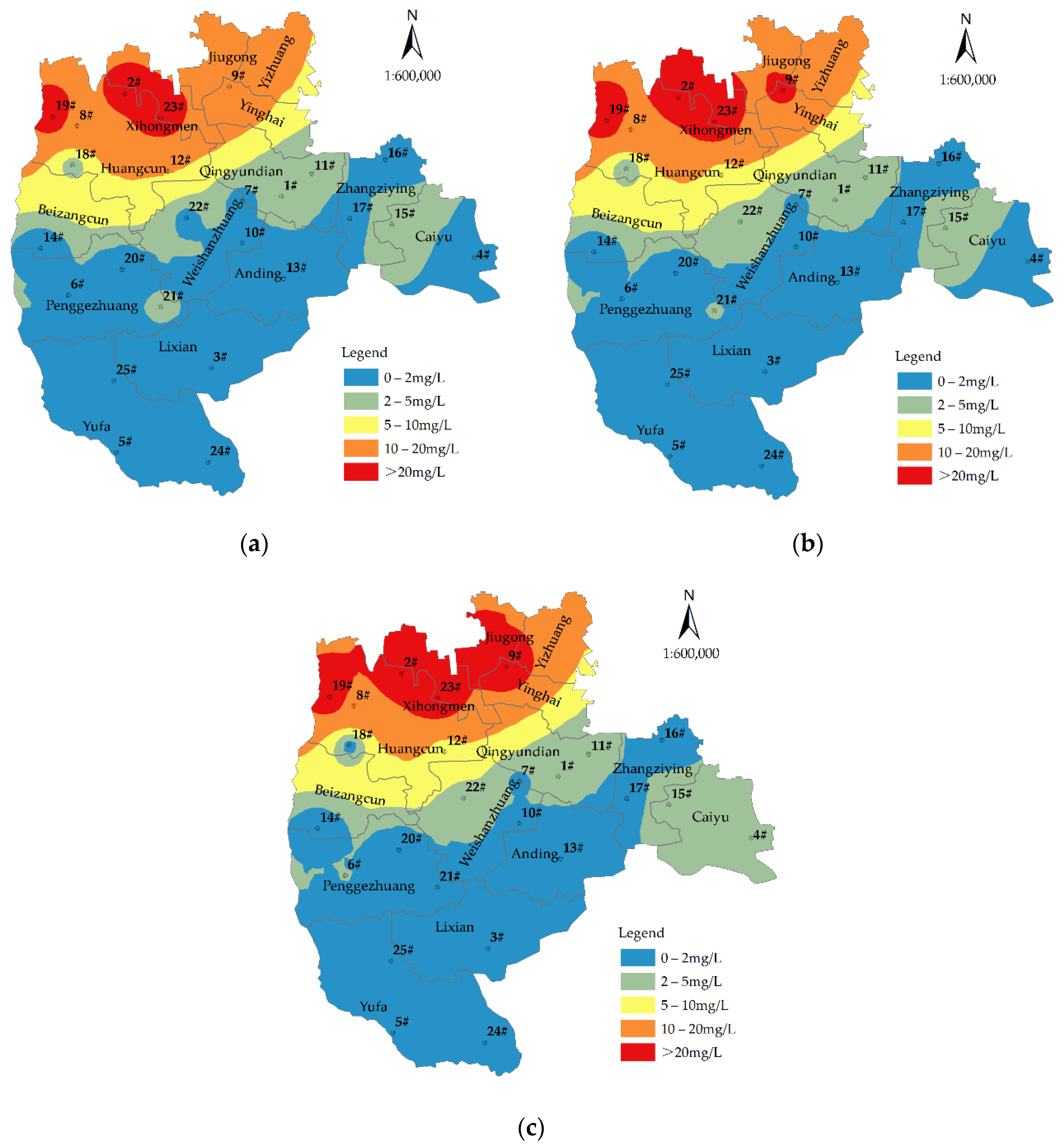
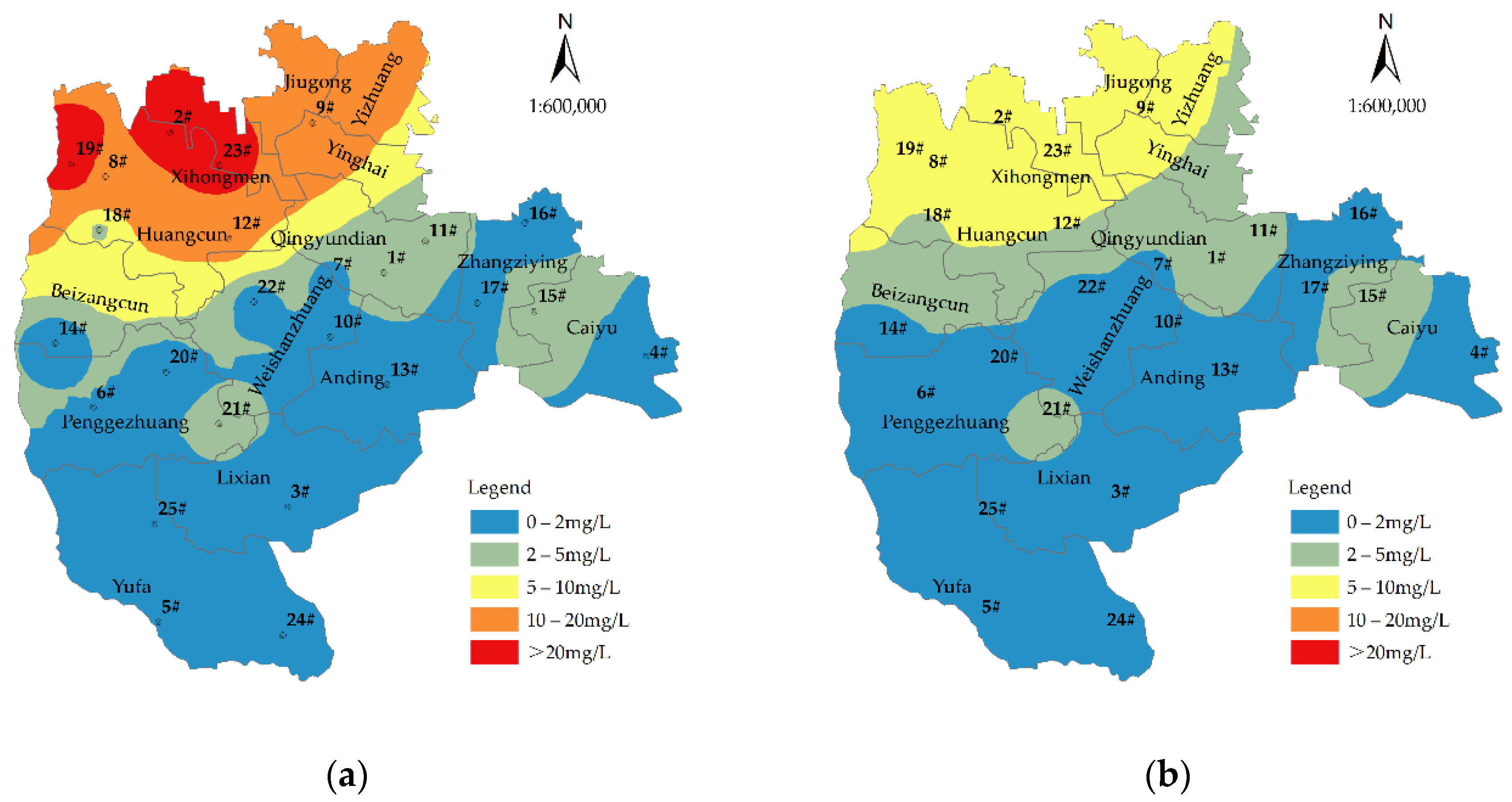
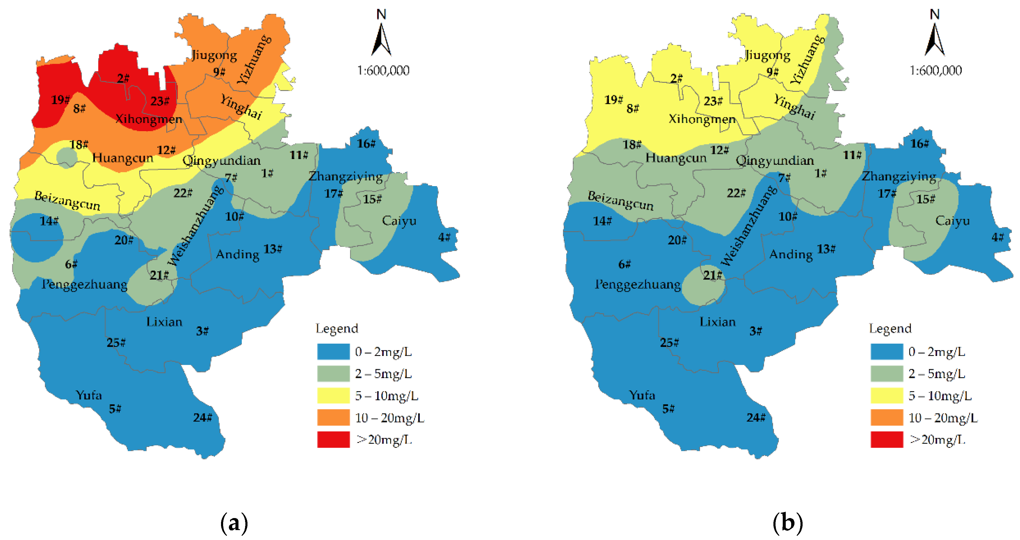
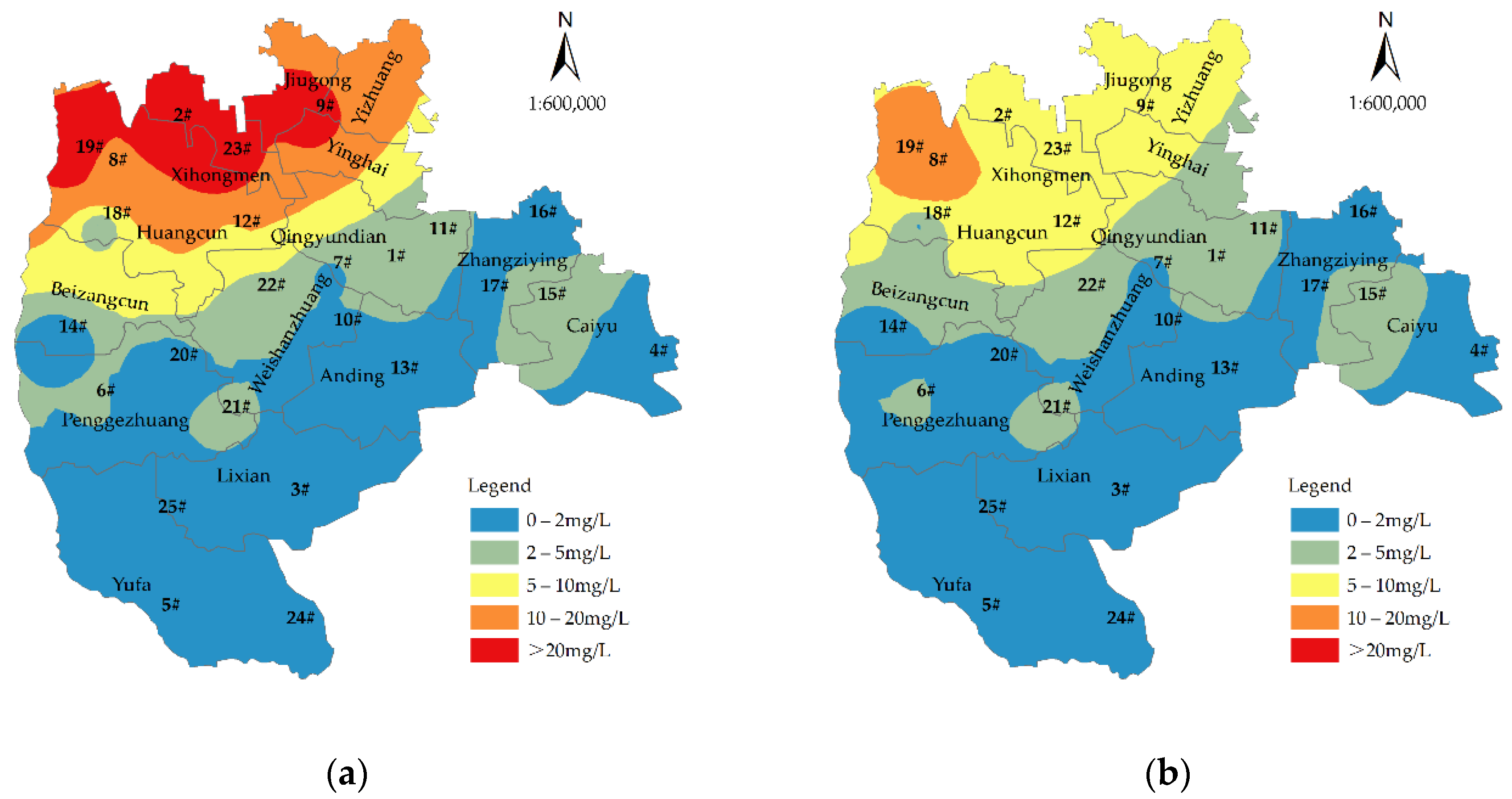
3.3. Changes in NO3-N Pollution before and after Optimal Regulation

It can be seen from the above that the best groundwater exploitation modes in wet, normal, and dry years were groundwater exploitation regime 3, groundwater exploitation regime 3, and groundwater exploitation regime 1, respectively. Taking 2025 as the example year, we used ArcGIS to draw the NO3-N concentration distribution map for the optimal groundwater exploitation regime in the wet year, normal year, and dry year scenarios, respectively (see Figure 11, Figure 12 and Figure 13).
Figure 11, Figure 12 and Figure 13 show that after the introduction of the optimal regimes, the predicted NO3-N concentration in 2025 dropped significantly, especially in the northern region. The NO3-N concentration in the wet year, normal year, and dry year scenarios decreased from 6.60 mg/L, 6.75 mg/L and 6.95 mg/L to 3.16 mg/L, 3.26 mg/L, and 3.84 mg/L respectively. The NO3-N concentration in the northern region decreased from 15.40 mg/L, 15.82 mg/L, and 16.42 mg/L to 6.31 mg/L, 6.61 mg/L, and 7.93 mg/L, respectively, for the different scenarios.

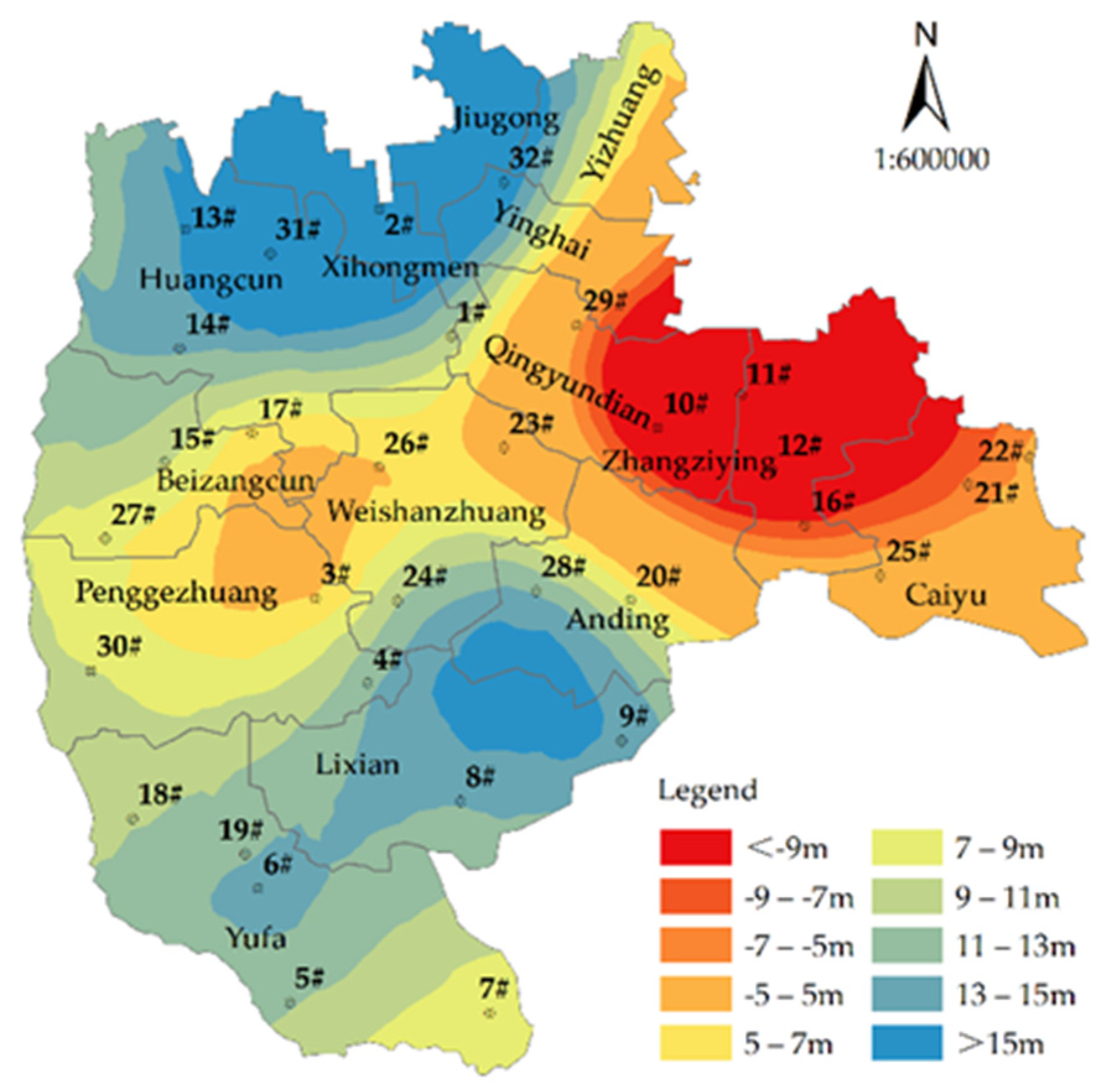
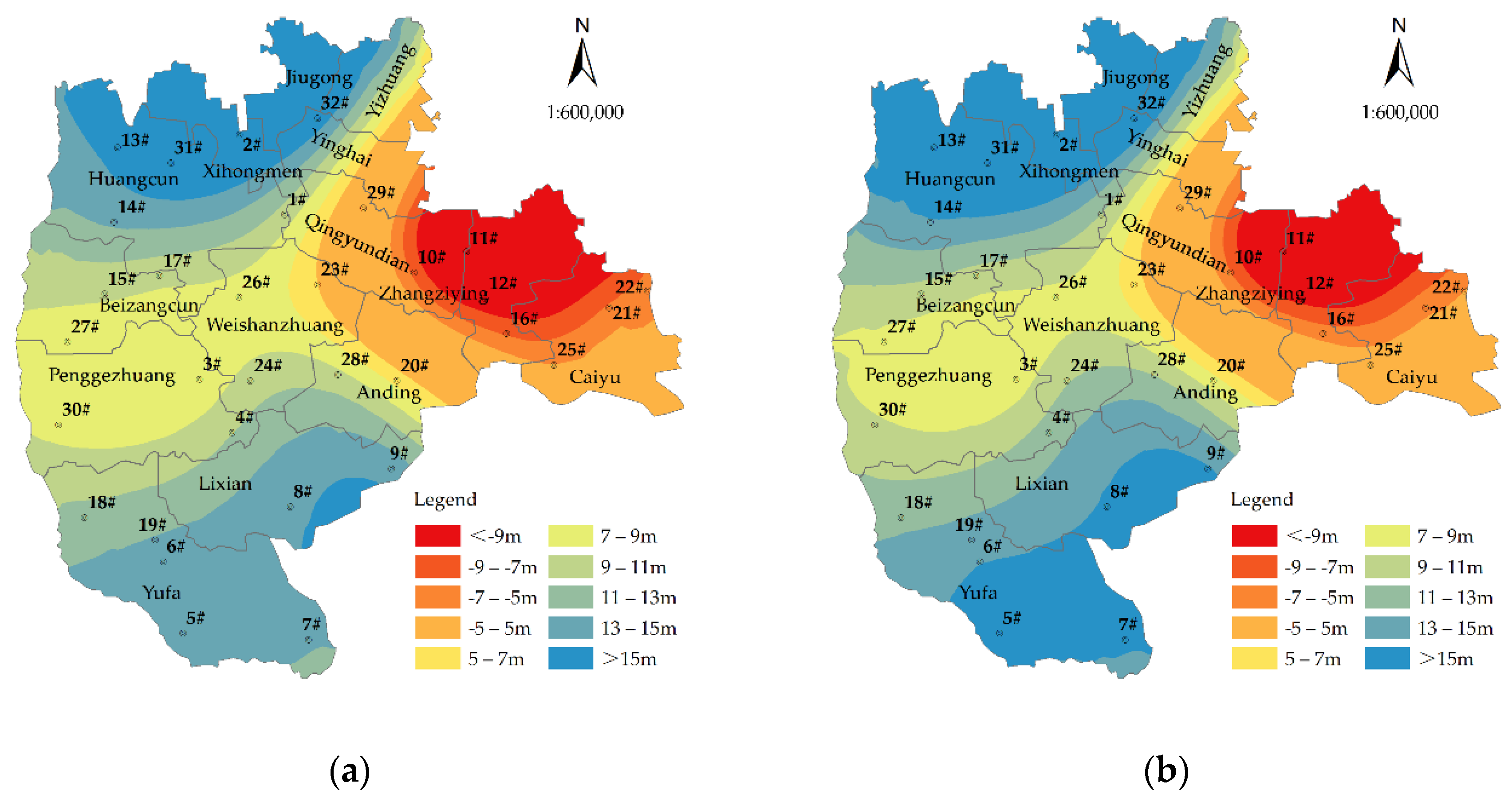
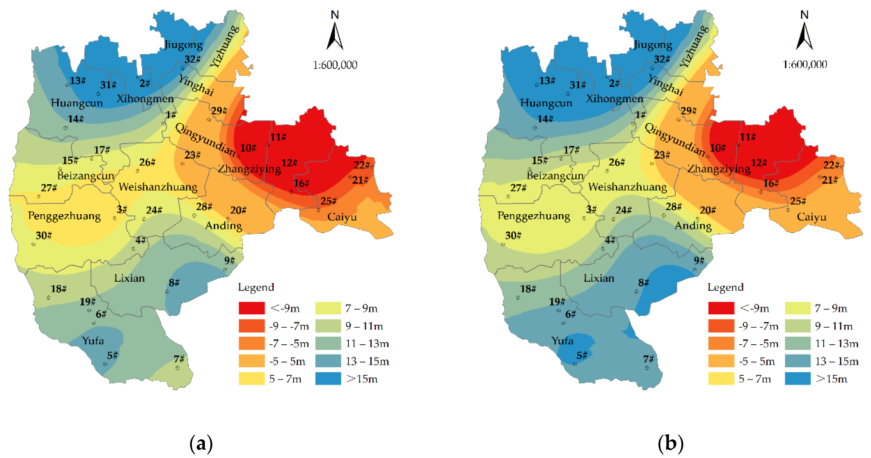
3.4. Changes in the Groundwater Table before and after Optimal Regulation

Taking 2025 as the example year, the Modflow model was used to simulate the changes in the groundwater table before and after optimal regulation. Taking 2020 as the initial groundwater table datum, the water resources from 2021 to 2025 were allocated according to groundwater exploitation regime 3, groundwater exploitation regime 3, and groundwater exploitation regime 1 in wet years, normal years, and dry years, respectively. The groundwater consumption before and after optimization was assumed to be the same as the groundwater exploitation volume before and after optimization. Taking 2021–2025 as the simulation period, the groundwater table distribution map for 2025 was obtained (Figure 14, Figure 15 and Figure 16).
It can be seen from Figure 14, Figure 15 and Figure 16 that the groundwater exploitation volume in the wet year was based on groundwater exploitation regime 3. Compared with the pre-optimization regime, the average groundwater table rose from 8.32 m to 9.31 m, meaning that the groundwater table rose by 0.99 m. From the perspective of the spatial change in the groundwater table, the groundwater table in the northern region rose from 13.61 m to 14.71 m, meaning that the groundwater table had risen by 1.10 m. The groundwater table in the central region rose by 0.74 m, and the groundwater table in the southern region rose by 1.12 m.
The groundwater exploitation mode in the normal year was based on groundwater exploitation regime 3. Compared with the preoptimization regime, the average groundwater table rose from 7.09 to 8.89 m, meaning that the groundwater table rose by 1.80 m. In more detail, the groundwater table in the northern region rose from 12.63 m to 14.38 m, a rise of 1.75 m. The groundwater table in the central region rose from 4.91 m to 6.47 m, a rise of 1.56 m. The groundwater table in the southern region rose from 3.72 m to 5.81 m, a rise of 2.09 m.
The groundwater exploitation mode in the dry year was based on groundwater exploitation mode 1. Compared with the pre-optimization regime, the average groundwater table rose from 6.10 m to 8.17 m, a rise of 2.07 m. The groundwater table in the northern region rose from 11.82 m to 13.80 m, a rise of 1.98 m; The groundwater level in the central region rose from 3.96 m to 5.80 m, a rise of 1.84 m; The groundwater level in the southern region rose from 2.49 m to 4.90 m, a rise of 2.41 m.
It can be seen from the above analysis that the groundwater level in the southern region increased the most, which might be related to the fact that the southern region is mainly agricultural. In this paper, after setting the guaranteed rate of agricultural water use and increasing the water supply of reclaimed water and surface water for agricultural water use, the exploitation of groundwater was reduced, resulting in rapid recovery of the groundwater level in the southern region.

4. Conclusions

In this paper, by combining GIS with machine-learning algorithms, water resources optimization technology, and groundwater numerical simulation, the groundwater quality and table in the Daxing District of Beijing were effectively optimized and controlled. The method developed here can provide theoretical and practical guidance for groundwater governance in areas with serious groundwater pollution and overexploitation. In more detail, the main conclusions of this paper are as follows:
(1)
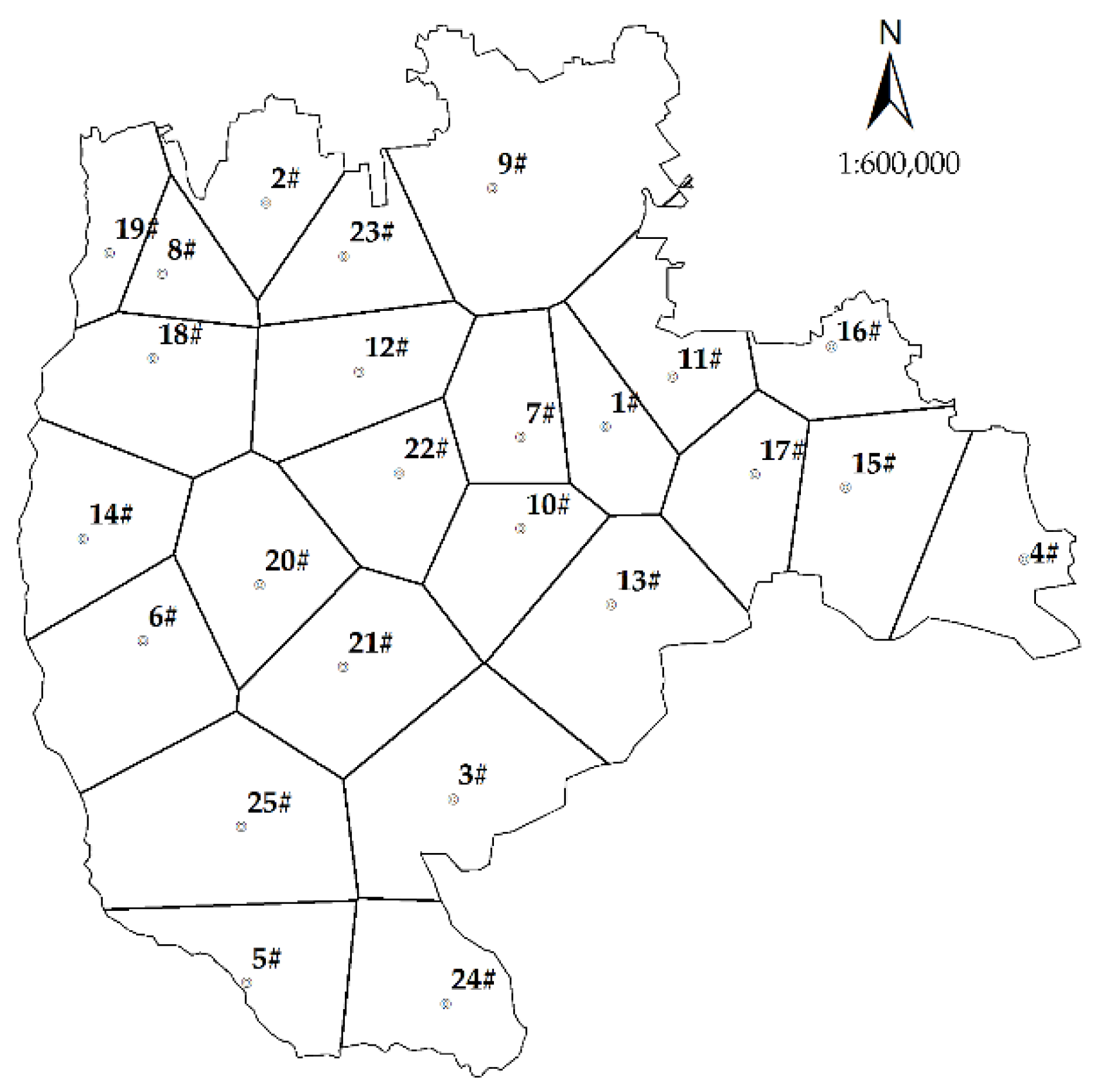
ArcGIS was used to generate Thiessen polygons around 25 water quality monitoring points. The regional analysis tool in ArcGIS was then used to extract the water consumption and economic development data for each polygon. Finally, three machine-learning algorithms were used to predict the NO3-N pollution under three different hydrological year scenarios for the Daxing District. The results show that LSTM had better accuracy than RF and SVR. Therefore, further research on the combination of GIS and LSTM has high theoretical and practical value.
(2)
According to our model’s predictions of future groundwater NO3-N pollution, this form of pollution shows an increasing trend in Daxing under the existing urban development regime. As compared with 2016–2020, the NO3-N pollution of groundwater over the period from 2021–2025 increased from 14.05 mg/L to 14.87 mg/L, 15.64 mg/L, and 16.54 mg/L in wet year, normal year, and dry year scenarios, respectively. It can be seen that the prediction pollution of pollution in the dry 2025 scenario was the most serious.
(3)
Taking 2025 as the example year for which to assess prospective mitigations of NO3-N pollution of groundwater, three new groundwater exploitation regimes were devised. A model for the optimal allocation of water resources was applied to the task of optimizing groundwater use under the three new regimes. The optimization results showed that of these new regimes, groundwater exploitation regime 3 should be adopted in a wet year and a normal year and that regime 1 should be adopted in a dry year.
(4)
Taking 2025 as the test year once more, we used ArcGIS to plot the changes in NO3-N pollution before and after optimization in wet year, normal year, and dry year scenarios. The results showed that the concentration of NO3-N decreased significantly after regime optimization. For the northern region of Daxing, which was the most polluted, the concentration of NO3-N decreased from 15.40 mg/L, 15.82 mg/L, and 16.42 mg/L to 6.31 mg/L, 6.61 mg/L, and 7.93 mg/L in the wet year, normal year, and dry year scenarios, respectively.
(5)
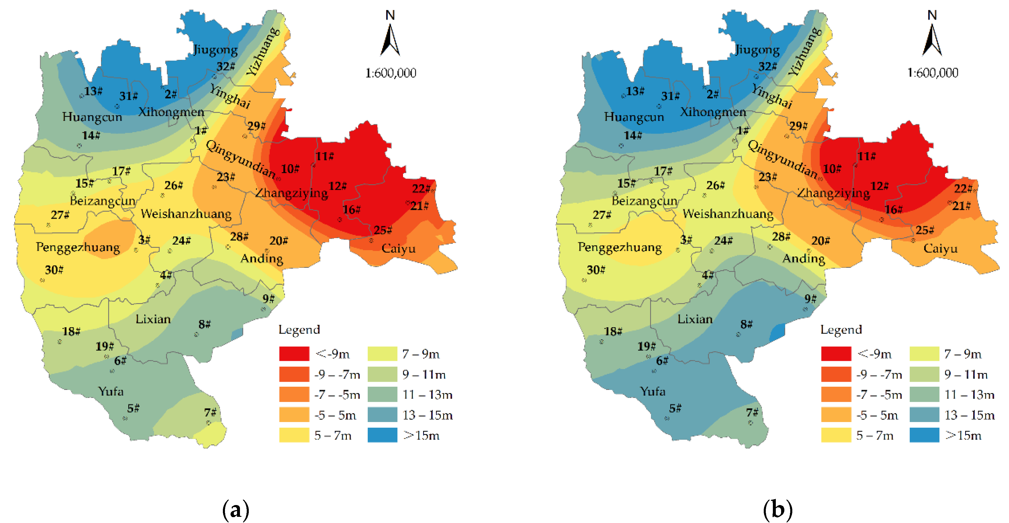
Taking 2025 as the test year for a third time, the Modflow model was used to simulate changes in the groundwater level before and after optimization and regulation. The results showed that the average groundwater table rose by 0.99 m, 1.80 m, and 2.07 m in the wet year, normal year, and dry year scenarios, respectively.
Because groundwater is buried deep underground, it is more difficult to control than surface water. To reduce groundwater overexploitation while ensuring water safety and adequacy of supply, the use of surface water, reclaimed water, and transferred water should be increased. To ensure groundwater quality, it is necessary to increase the supervision of industries with large emissions of pollutants. To achieve both ends, it is desirable to gradually eliminate or reform industries that currently have high water consumption and/or high pollution emissions. Domestic and industrial water should be fully collected and treated in a centralized manner, and its direct discharge into water bodies should be forbidden.
With the rapid development of both society and the economy, many countries and regions have problems with water shortage and water environment pollution. Especially in areas where surface water is scarce and groundwater is an important water source, achieving sustainable utilization of groundwater resources is of great significance to the development and stability of these areas, especially against the background of the increasing frequency of extreme weather in the world. By combining geographic information technology with machine prediction models, water resource optimization technology, and groundwater numerical simulation, this paper optimizes and controls the groundwater quality and table in the study area, achieving good results. Because of its powerful analytical functions, GIS is of great significance in under-standing and grasping temporal and spatial variations in groundwater. In addition, machine learning algorithms have great capacity to generate clear results from complex data. Therefore, it is of great help in realizing the management, supervision, and regulation of groundwater to combine GIS with machine learning algorithms. This paper can provide new ideas and methods for the sustainable utilization of groundwater in areas with both serious groundwater overexploitation and serious groundwater pollution.

Supplementary Materials

The following supporting information can be downloaded at: https://www.mdpi.com/article/10.3390/ijgi11100501/s1, Table S1: Errors between the calculated NO3-N concentration values and the monitored NO3-N concentration values for the three machine learning algorithms during the validation period; Table S2: Optimal allocation of water resources under wet year in 2025; Table S3: Optimal allocation of water resources under normal year in 2025; Table S4: Optimal allocation of water resources under dry year in 2025.

Author Contributions

Conceptualization, Baohui Men and Shiyang Yin; methodology, Chen Li; software, Chen Li; Teng Zhang and Ling Wei; validation, Chen Li; formal analysis, Chen Li; investigation, Chen Li; resources, Chen Li; data curation, Chen Li; writing—original draft preparation, Chen Li; writing—review and editing, Chen Li; visualization, Chen Li; supervision, Baohui Men and Shiyang Yin; project administration, Baohui Men and Shiyang Yin; funding acquisition, Baohui Men and Shiyang Yin. All authors have read and agreed to the published version of the manuscript.

Funding

This research was funded by the Ministry of Education of the People’s Republic of China (2019MS028) and the Ministry of Science and Technology of the People’s Republic of China (2016YFC0401406).

Institutional Review Board Statement

Not applicable.

Informed Consent Statement

Not applicable.

Data Availability Statement

Data can be made available upon request. The statistical data can be found here: http://swj.beijing.gov.cn/zwgk (accessed on 20 July 2022).

Acknowledgments

Thanks for the support of the above funding entities and the Laboratory of College of Water Resources and Hydropower Engineering, North China Electric Power University.

Conflicts of Interest

The authors declare no conflict of interest.

References

  1. Wang, S.J.; Ma, H.T.; Zhao, Y.B. Exploring the relationship between urbanization and the eco-environment-A case study of Beijing-Tianjin-Hebei region. Ecol. Indic. 2014, 45, 171–183. [Google Scholar] [CrossRef]
  2. Wu, W.J.; Zhao, S.Q.; Zhu, C.; Jiang, J.L. A comparative study of urban expansion in Beijing, Tianjin and Shijiazhuang over the past three decades. Landsc. Urban Plan. 2015, 134, 93–106. [Google Scholar] [CrossRef]
  3. Hubacek, K.; Guan, D.B.; Barrett, J.; Wiedmann, T. Environmental implications of urbanization and lifestyle change in China: Ecological and Water Footprints. J. Clean Prod. 2009, 17, 1241–1248. [Google Scholar] [CrossRef]
  4. Chen, B.B.; Gong, H.L.; Li, X.J.; Lei, K.C.; Zhu, L.; Gao, M.L.; Zhou, C.F. Characterization and causes of land subsidence in Beijing, China. Int. J. Remote Sens. 2017, 38, 808–826. [Google Scholar] [CrossRef]
  5. Chen, J.; Tang, C.; Sakura, Y.; Yu, J.; Fukushima, Y. Nitrate pollution from agriculture in different hydrogeological zones of the regional groundwater flow system in the North China Plain. Hydrogeol. J. 2005, 13, 481–492. [Google Scholar] [CrossRef]
  6. Malczewski, J. GIS-based land-use suitability analysis: A critical overview. Prog. Plann. 2004, 62, 3–65. [Google Scholar] [CrossRef]
  7. Singh, A. Managing the water resources problems of irrigated agriculture through geospatial techniques: An overview. Agr. Water Manag. 2016, 174, 2–10. [Google Scholar] [CrossRef]
  8. Yang, X.J. Remote sensing and GIS applications for estuarine ecosystem analysis: An overview. Int. J. Remote Sens. 2005, 26, 5347–5356. [Google Scholar] [CrossRef]
  9. Garg, J.K. Wetland assessment, monitoring and management in India using geospatial techniques. J. Env. Manag. 2015, 148, 112–123. [Google Scholar] [CrossRef]
  10. Zhou, J.; Wang, Y.Y.; Xiao, F.; Wang, Y.Y.; Sun, L.J. Water Quality Prediction Method Based on IGRA and LSTM. Water 2018, 10, 1148. [Google Scholar] [CrossRef] [Green Version]
  11. Parmar, K.S.; Bhardwaj, R. Water quality management using statistical analysis and time-series prediction model. Appl. Water Sci. 2014, 4, 425–434. [Google Scholar] [CrossRef]
  12. Asgari, G.; Gholi, M.N.; Salari, M.; Asgharnia, H.; Darvishmotevalli, M.; Faraji, H.; Moradnia, M. Forecasting nitrate concentration in babol groundwater resources using the grey model (1,1). Int. J. Environ. Health Eng. 2020, 9, 16. [Google Scholar] [CrossRef]
  13. Parmar, K.S.; Bhardwaj, R. River Water Prediction Modeling Using Neural Networks, Fuzzy and Wavelet Coupled Model. Water Resour. Manag. 2015, 29, 17–33. [Google Scholar] [CrossRef]
  14. Guner, E.D.; Kuvvetli, Y. Analysis of groundwater quality for drinking purposes using combined artificial neural networks and fuzzy logic approaches. Desalin Water Treat. 2020, 174, 143–151. [Google Scholar] [CrossRef]
  15. Li, J.; Li, X.; Lv, N.Q.; Yang, Y.; Xi, B.D.; Li, M.X.; Bai, S.G.; Liu, D. Quantitative assessment of groundwater pollution intensity on typical contaminated sites in China using grey relational analysis and numerical simulation. Environ. Earth Sci. 2015, 74, 3955–3968. [Google Scholar] [CrossRef]
  16. Yang, W.; Zhang, K.N.; Chen, Y.G.; Zhou, X.Z.; Jin, F.X. Prediction on contaminant migration in aquifer of fractured granite substrata of landfill. J. Cent. South Univ. 2013, 20, 3193–3201. [Google Scholar] [CrossRef]
  17. Agrawal, P.; Sinha, A.; Kumar, S.; Agarwal, A.; Banerjee, A.; Villuri, V.; Annavarapu, C.; Dwivedi, R.; Dera, V.; Sinha, J.; et al. Exploring Artificial Intelligence Techniques for Groundwater Quality Assessment. Water 2021, 13, 1172. [Google Scholar] [CrossRef]
  18. Ahmadi, A.; Olyaei, M.; Heydari, Z.; Emami, M.; Zeynolabedin, A.; Ghomlaghi, A.; Daccache, A.; Fogg, G.E.; Sadegh, M. Groundwater Level Modeling with Machine Learning: A Systematic Review and Meta-Analysis. Water 2022, 14, 949. [Google Scholar] [CrossRef]
  19. Patle, G.T.; Singh, D.K.; Sarangi, A.; Rai, A.; Khanna, M.; Sahoo, R.N. Time Series Analysis of Groundwater Levels and Projection of Future Trend. J. Geol. Soc. India 2015, 85, 232–242. [Google Scholar] [CrossRef]
  20. Zhang, X.; Li, P.; Bin Li, Z.; Yu, G.Q. Soil water-salt dynamics state and associated sensitivity factors in an irrigation district of the loess area: A case study in the Luohui Canal Irrigation District, China. Environ. Earth Sci. 2017, 76, 715. [Google Scholar] [CrossRef]
  21. Nazari, H.; Taghavi, B.; Hajizadeh, F. Groundwater salinity prediction using adaptive neuro-fuzzy inference system methods: A case study in Azarshahr, Ajabshir and Maragheh plains, Iran. Environ. Earth Sci. 2021, 80, 152. [Google Scholar] [CrossRef]
  22. Liu, F.M.; Yi, S.P.; Ma, H.Y.; Huang, J.Y.; Tang, Y.K.; Qin, J.B.; Zhou, W.H. Risk assessment of groundwater environmental contamination: A case study of a karst site for the construction of a fossil power plant. Environ. Sci. Pollut. R. 2019, 26, 30561–30574. [Google Scholar] [CrossRef] [PubMed]
  23. Aghlmand, R.; Abbasi, A. Application of MODFLOW with Boundary Conditions Analyses Based on Limited Available Observations: A Case Study of Birjand Plain in East Iran. Water 2019, 11, 1904. [Google Scholar] [CrossRef]
  24. Kouadri, S.; Elbeltagi, A.; Islam, A.; Kateb, S. Performance of machine learning methods in predicting water quality index based on irregular data set: Application on Illizi region (Algerian southeast). Appl. Water Sci. 2021, 11, 190. [Google Scholar] [CrossRef]
  25. Sun, J.; Wang, G.H. Geographic Information System Technology Combined with Back Propagation Neural Network in Groundwater Quality Monitoring. Isprs. Int. J. Geo-Inf. 2020, 9, 736. [Google Scholar] [CrossRef]
  26. Setshedi, K.J.; Mutingwende, N.; Ngqwala, N.P. The Use of Artificial Neural Networks to Predict the Physicochemical Characteristics of Water Quality in Three District Municipalities, Eastern Cape Province, South Africa. Int. J. Env. Res. Pub. He. 2021, 18, 5248. [Google Scholar] [CrossRef] [PubMed]
  27. Yoon, H.; Hyun, Y.; Ha, K.; Lee, K.K.; Kim, G.B. A method to improve the stability and accuracy of ANN- and SVM-based time series models for long-term groundwater level predictions. Comput. Geosci. 2016, 90, 144–155. [Google Scholar] [CrossRef]
  28. Liang, Z.H.; Liu, Y.P.; Hu, H.C.; Li, H.Q.; Ma, Y.Q.; Khan, M. Combined Wavelet Transform with Long Short-Term Memory Neural Network for Water Table Depth Prediction in Baoding City, North China Plain. Front. Environ. Sci. 2021, 78, 565. [Google Scholar] [CrossRef]
  29. Gupta, P.K.; Maiti, S. Enhancing data-driven modeling of fluoride concentration using new data mining algorithms. Environ. Earth Sci. 2022, 81, 89. [Google Scholar] [CrossRef]
  30. Aldhyani, T.H.H.; Al-Yaari, M.; Alkahtani, H.; Maashi, M.; Algalil, F.A. Water Quality Prediction Using Artificial Intelligence Algorithms. Appl. Bionics. Biomech. 2020, 2020, 6659314. [Google Scholar] [CrossRef]
  31. Kumar, S.; Pati, J. Assessment of groundwater arsenic contamination using machine learning in Varanasi, Uttar Pradesh, India. J. Water Health 2022, 20, 829–848. [Google Scholar] [CrossRef] [PubMed]
  32. Islam, A.R.M.T.; Pal, S.C.; Chakrabortty, R.; Idris, A.M.; Salam, R.; Islam, M.S.; Zahid, A.; Shahid, S.; Ismail, Z.B. A coupled novel framework for assessing vulnerability of water resources using hydrochemical analysis and data-driven models. J. Clean Prod. 2022, 336, 130407. [Google Scholar] [CrossRef]
  33. Rodriguez-Galiano, V.; Mendes, M.P.; Garcia-Soldado, M.J.; Chica-Olmo, M.; Ribeiro, L. Predictive modeling of groundwater nitrate pollution using Random Forest and multisource variables related to intrinsic and specific vulnerability: A case study in an agricultural setting (Southern Spain). Sci. Total Environ. 2014, 476–477, 189–206. [Google Scholar] [CrossRef] [PubMed]
  34. Norouzi, H.; Moghaddam, A.A. Groundwater quality assessment using random forest method based on groundwater quality indices (case study: Miandoab plain aquifer, NW of Iran). Arab. J. Geosci. 2020, 13, 912. [Google Scholar] [CrossRef]
  35. Arabgol, R.; Sartaj, M.; Asghari, K. Predicting Nitrate Concentration and Its Spatial Distribution in Groundwater Resources Using Support Vector Machines (SVMs) Model. Environ. Model Assess. 2016, 21, 71–82. [Google Scholar] [CrossRef]
  36. Dixon, B. A case study using support vector machines, neural networks and logistic regression in a GIS to identify wells contaminated with nitrate-N. Hydrogeol. J. 2009, 17, 1507–1520. [Google Scholar] [CrossRef]
  37. Xiao, Y.; Liu, K.; Hao, Q.; Xiao, D.; Zhu, Y.; Yin, S.; Zhang, Y. Hydrogeochemical insights into the signatures, genesis and sustainable perspective of nitrate enriched groundwater in the piedmont of Hutuo watershed, China. Catena 2022, 212, 106020. [Google Scholar] [CrossRef]
  38. Dai, C.; Tang, J.; Li, Z.; Duan, Y.; Qu, Y.; Yang, Y.; Lyu, H.; Zhang, D.; Wang, Y. Index System of Water Resources Development and Utilization Level Based on Water-Saving Society. Water 2022, 14, 802. [Google Scholar] [CrossRef]
  39. Liu, J.; Zhao, X.; Yang, H.; Liu, Q.; Xiao, H.; Cheng, G. Assessing China’s “developing a water-saving society” policy at a river basin level: A structural decomposition analysis approach. J. Clean. Prod. 2018, 190, 799–808. [Google Scholar] [CrossRef]
  40. Du, M.; Liao, L.; Wang, B.; Chen, Z. Evaluating the effectiveness of the water-saving society construction in China: A quasi-natural experiment. J. Environ. Manag. 2021, 277, 111394. [Google Scholar] [CrossRef]
  41. Hochreiter, S. The vanishing gradient problem during learning recurrent neural nets and problem solutions. Int. J. Uncertain. Fuzziness Knowl.-Based Syst. 1998, 6, 107–116. [Google Scholar] [CrossRef]
  42. Hochreiter, S.; Schmidhuber, J. Long Short-Term Memory. Neural Comput. 1997, 9, 1735–1780. [Google Scholar] [CrossRef] [PubMed]
  43. Breiman, L. Random Forests. Mach. Learn 2001, 45, 5–32. [Google Scholar] [CrossRef]
  44. Das, S.; Chakraborty, R.; Maitra, A. A random forest algorithm for nowcasting of intense precipitation events. Adv. Space Res. 2017, 60, 1271–1282. [Google Scholar] [CrossRef]
  45. Nashwan, M.S.; Shahid, S. Symmetrical uncertainty and random forest for the evaluation of gridded precipitation and temperature data. Atmos. Res. 2019, 230, 104632. [Google Scholar] [CrossRef]
  46. Wang, X.; Zhong, Y. Statistical learning theory and state of the art in SVM. In Proceedings of the Second IEEE International Conference on Cognitive Informatics, 2003. Proceedings, London, UK, 18–20 August 2003; pp. 55–59. [Google Scholar] [CrossRef]
  47. Ngatchou, P.; Zarei, A.; El-Sharkawi, A. Pareto Multi Objective Optimization. In Proceedings of the 13th International Conference on, Intelligent Systems Application to Power Systems, Arlington, VA, USA, 6–10 November 2005; pp. 84–91. [Google Scholar] [CrossRef]
  48. Deb, K.; Pratap, A.; Agarwal, S.; Meyarivan, T. A fast and elitist multiobjective genetic algorithm: NSGA-II. IEEE T. Evolut. Comput. 2002, 6, 182–197. [Google Scholar] [CrossRef]
  49. Alagha, J.S.; Said, M.A.M.; Mogheir, Y. Modeling of nitrate concentration in groundwater using artificial intelligence approach—a case study of Gaza coastal aquifer. Environ. Monit. Assess. 2014, 186, 35–45. [Google Scholar] [CrossRef]
  50. Nadali, A.; Ebrahim, Z.; Morteza, H.; Ali, A.B.; Gholamreza, G.; Ahmad, R.Y.; Mohammad, J.M. Water quality assessment and zoning analysis of Dez eastern aquifer by Schuler and Wilcox diagrams and GIS. Desalin. Water Treat. 2016, 57, 23686–23697. [Google Scholar]
Figure 1. Geographic map of the study area.
Ijgi 11 00501 g001
Figure 2. Section A–A′ of the study area.
Ijgi 11 00501 g002
Figure 3. The relationship between the groundwater table and river.
Ijgi 11 00501 g003
Figure 4. Hydrogeological parameter partition map of Daxing.
Ijgi 11 00501 g004
Figure 5. Distribution map of current groundwater table in study area, taking the year 2020 as an example.
Ijgi 11 00501 g005
Figure 6. The ratio between the calculated level and the actual level of the groundwater table during the verification period (the elevation reference system is the 1956 Yellow Sea Elevation System of China).
Ijgi 11 00501 g006
Figure 7. Spatial distribution of NO3-N concentration in Daxing groundwater from 2006 to 2020: (a) 2006–2010; (b) 2011–2015; (c) 2016–2020.
Ijgi 11 00501 g007
Figure 8. Thiessen polygons based on the 25 groundwater quality monitoring points in Daxing and the district boundaries.
Ijgi 11 00501 g008
Figure 9. The ratio between the calculated and actual values of NO3-N concentration for the three machine learning algorithms during the validation period: (a) LSTM; (b) RF; (c) SVR.
Ijgi 11 00501 g009aIjgi 11 00501 g009b
Figure 10. Spatial distribution of predicted NO3-N concentrations from 2021 to 2025: (a) 2021–2025 (wet year); (b) 2021–2025 (normal year); (c) 2021–2025 (dry year).
Ijgi 11 00501 g010
Figure 11. Changes of NO3-N concentration in a wet year 2025 (groundwater exploitation regime 3): (a) before optimization and (b) after optimization.
Ijgi 11 00501 g011
Figure 12. Changes of NO3-N concentration in a normal year 2025 (groundwater exploitation regime 3): (a) before optimization and (b) after optimization.
Ijgi 11 00501 g012
Figure 13. Changes of NO3-N concentration in a dry year 2025 (groundwater exploitation regime 1): (a) before optimization and (b) after optimization,.
Ijgi 11 00501 g013
Figure 14. Changes of groundwater table in a wet 2025 (groundwater exploitation regime 3): (a) before optimization and (b) after optimization.
Ijgi 11 00501 g014
Figure 15. Changes of groundwater table in normal year 2025 (groundwater exploitation regime 3): (a) before optimization and (b) after optimization.
Ijgi 11 00501 g015
Figure 16. Changes of groundwater table in a dry 2025 (groundwater exploitation regime 1): (a) before optimization and (b) after optimization.
Ijgi 11 00501 g016
Table 1. Hydrogeological parameters of Daxing.
Parameter Partition NumberZone Area (km2)Permeability Coefficient K (m/d)Specific Yield μ
Zone I532.1015–250.20–0.26
Zone II384.998–100.13–0.20
Zone III118.9110–150.10–0.15
Table 2. Calculation results of groundwater source and sink items in Daxing District from 2015 to 2020.
Source and Sink Items2015
(104 m3)
2016
(104 m3)
2017
(104 m3)
2018
(104 m3)
2019
(104 m3)
2020
(104 m3)
Atmospheric precipitation infiltration recharge15,699.3020,928.1015,955.2314,423.3012,782.1714,346.22
River infiltration recharge2230.103032.802278.902060.091825.692049.08
Well irrigation return recharge2732.102580.602388.002143.802164.001472.00
Groundwater lateral inflow376.20530.00403.9024365.12323.58363.17
Artificial exploitation21,672.5021,390.7320,618.6318,791.6219,493.9815,507.55
Groundwater lateral outflow103.00145.10108.3597.9586.8097.43
Changes in groundwater storage−737.805535.67299.05102.74−2485.342625.49
Table 3. Hydrogeological parameters derived for the three aquifer zones of Daxing.
Parameter ZoneZone Area (km2)Permeability Coefficient K (m/d)Specific Yield μ
Zone I532.1015.40.25
Zone II384.999.950.20
Zone III118.9111.70.105
Table 4. The available groundwater volumes for Daxing under groundwater exploitation regimes 1–3.
Hydrological Year TypeThe Maximum Available Groundwater Volume before Reduction
(104 m3)
Groundwater Exploitation Regime 1
(104 m3)
Groundwater Exploitation Regime 2
(104 m3)
Groundwater Exploitation Regime 3
(104 m3)
Reduction in the Amount of Groundwater ExtractionThe Available Groundwater VolumeReduction in the Amount of Groundwater ExtractionThe Available Groundwater VolumeReduction in the Amount of Groundwater ExtractionThe Available Groundwater Volume
Wet year22,450.66981.4621,469.204798.7317,651.935644.8216,805.84
Normal year18,086.541540.9516,545.594868.9813,217.565578.2012,508.34
Dry year1,4931.442549.6812,381.765037.49894.045611.839319.61
Table 5. Optimal evaluation of groundwater exploitation modes.
Hydrological Year TypeGroundwater Exploitation RegimeWater Shortage
(104 m3)
Amount of Groundwater Used
(104 m3)
The Maximum Amount of Groundwater Available
(104 m3)
Groundwater Utilization RateNO3-N Maximum Concentration (mg/L)
Wet yearCurrent groundwater exploitation regime021,456.0922,450.6695.57%27.15
Groundwater exploitation regime 1016,630.1122,450.6674.07%13.32
Groundwater exploitation regime 2016,630.1122,450.6674.07%12.00
Groundwater exploitation regime 3016,630.1122,450.6674.07%10.64
Normal yearCurrent groundwater exploitation regime021,456.0918,086.54118.63%28.24
Groundwater exploitation regime 1016,545.5918,086.5491.48%17.63
Groundwater exploitation regime 2013,217.5618,086.5473.08%11.52
Groundwater exploitation regime 3012,508.3418,086.5469.16%11.02
Dry yearCurrent groundwater exploitation regime023,038.3914,931.44154.29%28.55
Groundwater exploitation regime 1012,381.7614,931.4482.92%17.72
Groundwater exploitation regime 2−2440.869894.0414,931.4466.26%10.85
Groundwater exploitation regime 3−3015.299319.6114,931.4462.42%10.14
Publisher’s Note: MDPI stays neutral with regard to jurisdictional claims in published maps and institutional affiliations.

