
Improving Road Surface Area Extraction via Semantic Segmentation with Conditional Generative Learning for Deep Inpainting Operations

 ,
,  ,
,  and
and 
Abstract
:1. Introduction
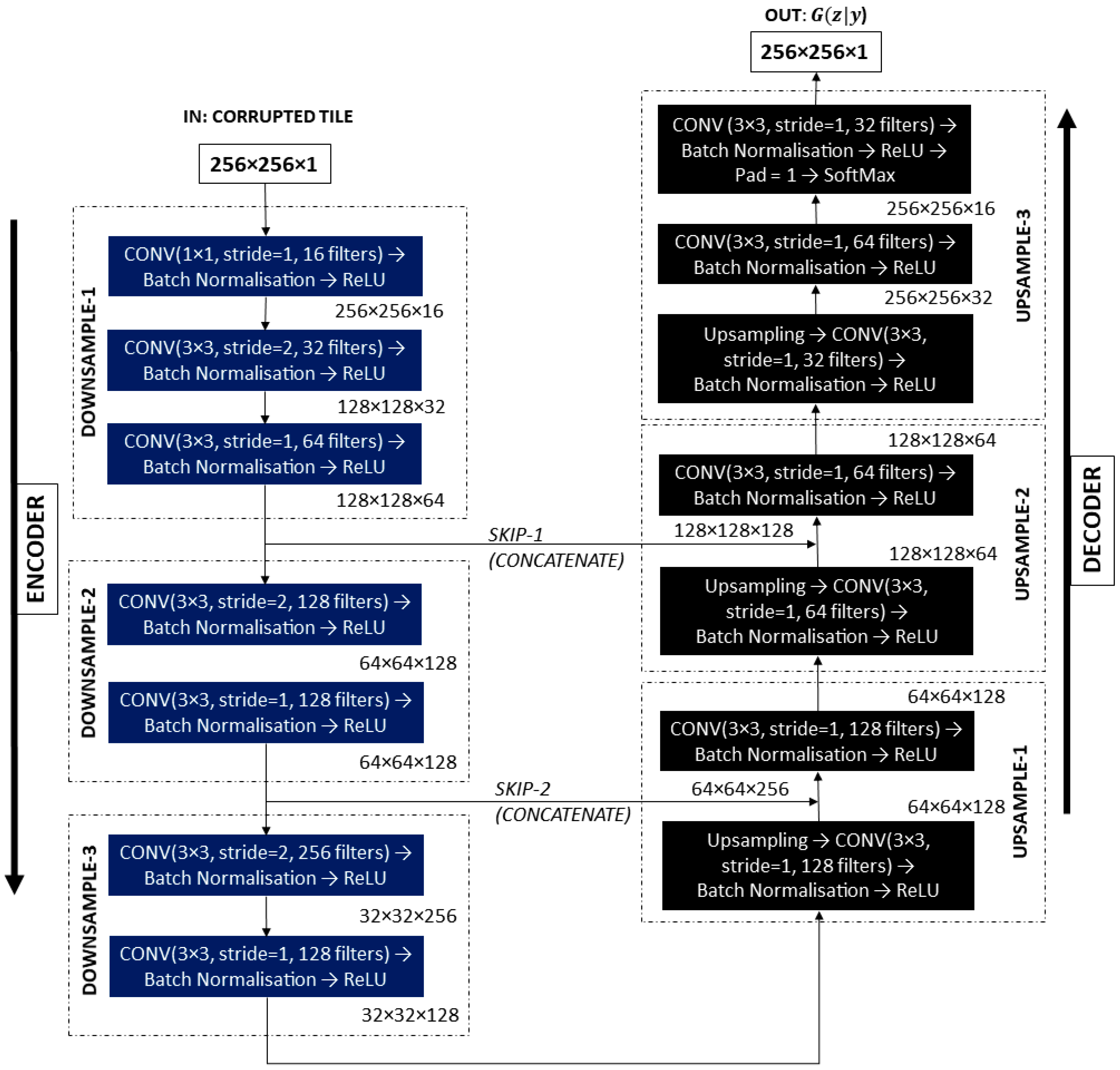
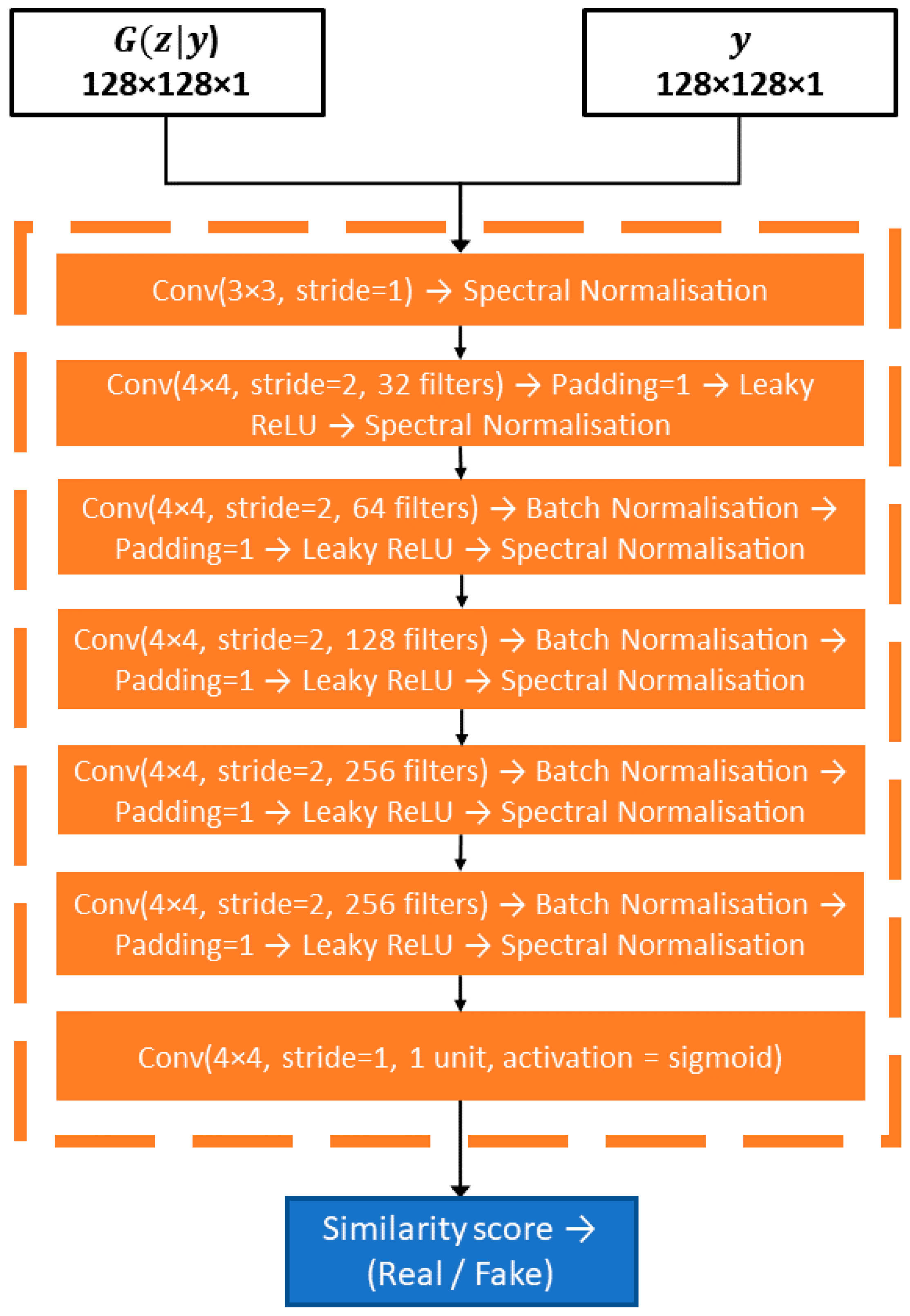
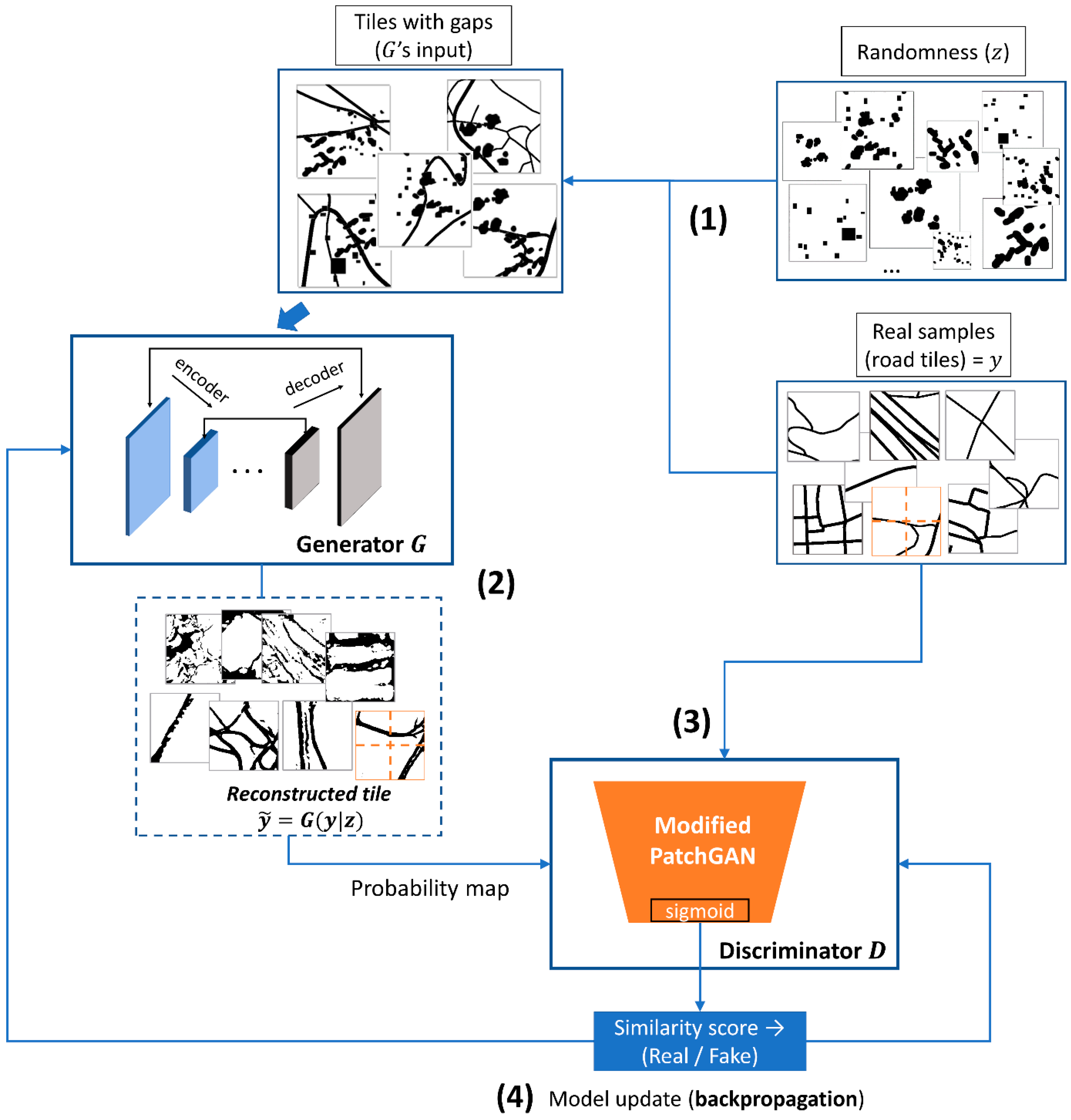
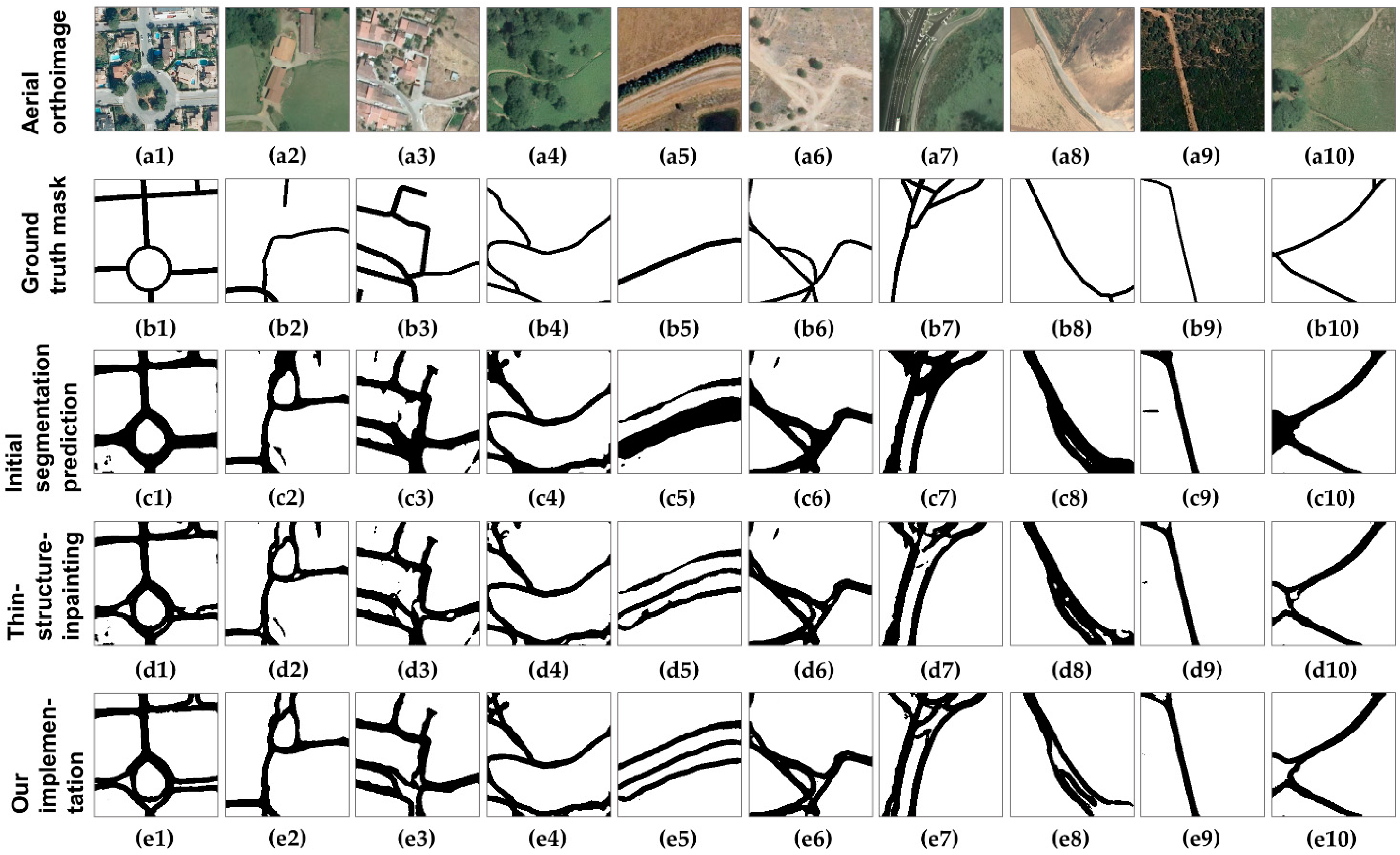
- We implemented a cGAN model for the deep inpainting task to improve the initial semantic segmentation predictions of roads. We proposed generator, , and discriminator, , architectures in order to make the training better suited for our learning objective. is a U-Net [13]-like network, heavily modified for computational efficiency, while is a modified PatchGAN [14], adapted to process images of 256 × 256 pixels.
- We trained the model on a new dataset composed of real segmentation maps of roads present in official cartography. Here, we applied randomness in the form of synthetic gaps to the input for training (which will result in many possible corrupted images [15]). This source of randomness applied to the conditional information allows to generate realistic images. We validated the model on a new test set composed of real semantic segmentation predictions obtained by a state-of-the-art semantic segmentation network (with U-Net as base architecture and SEResNeXt50 [16] as segmentation backbone). We performed this operation at large-scale, with an intent to obtain a production model capable of successfully reducing human participation in the road extraction task.
- We studied the appropriateness of applying generative learning with inpainting operations for the task of road post-processing by evaluating the model’s ability in generating new samples from the learned domain and conducting metrical comparison and perceptual validation operations. The cGAN proposed achieved a maximum increase of 1.28% over the IoU score obtained by the semantic segmentation model.
2. Related Work
3. Problem Description
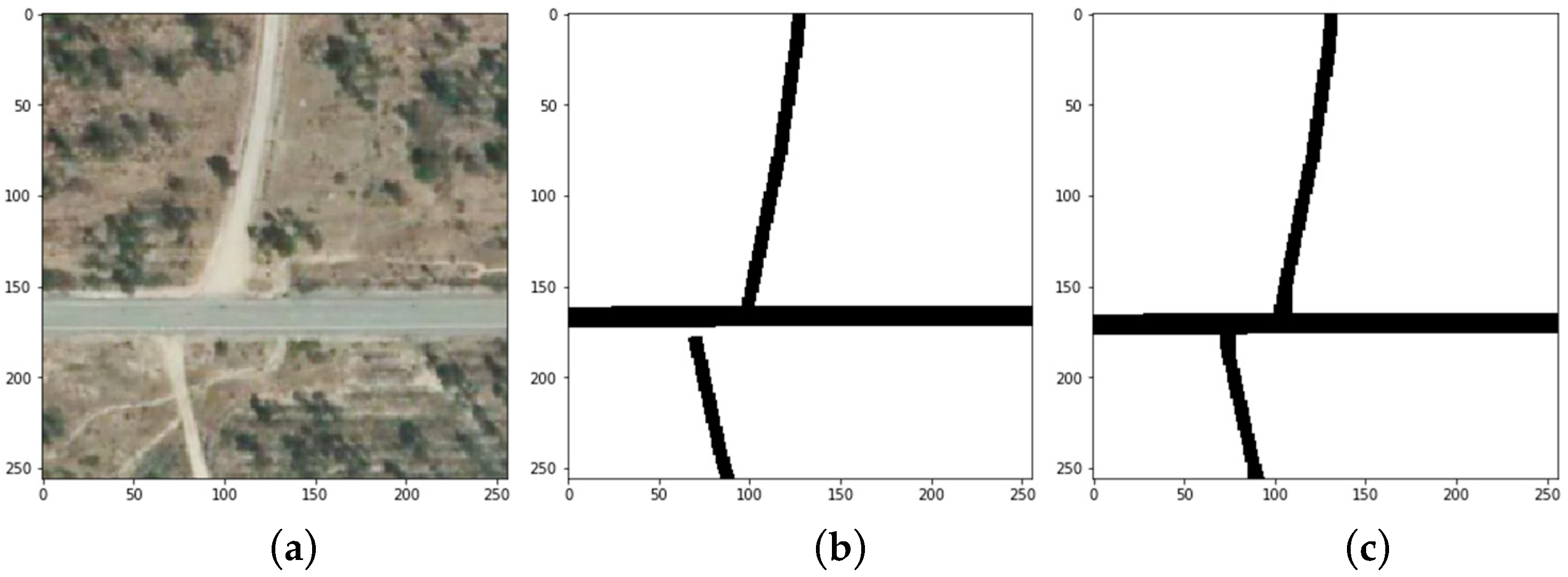
4. Data
5. cGAN for Post-Processing Road Predictions via Deep Inpainting Operations
5.1. Generator
5.2. Discriminator
5.3. Learning Process
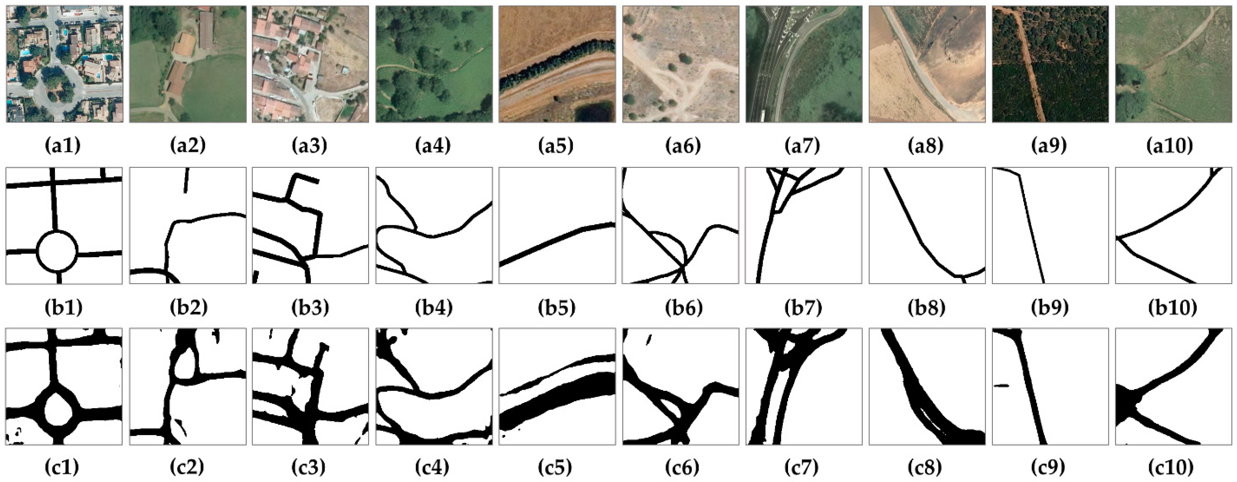
6. Experiments and Analysis of the Results
7. Conclusions
Author Contributions
Funding
Institutional Review Board Statement
Informed Consent Statement
Data Availability Statement
Acknowledgments
Conflicts of Interest
References
- Cira, C.-I.; Alcarria, R.; Manso-Callejo, M.-Á.; Serradilla, F. A Deep Learning-Based Solution for Large-Scale Extraction of the Secondary Road Network from High-Resolution Aerial Orthoimagery. Appl. Sci. 2020, 10, 7272. [Google Scholar] [CrossRef]
- Hu, F.; Xia, G.-S.; Hu, J.; Zhang, L. Transferring Deep Convolutional Neural Networks for the Scene Classification of High-Resolution Remote Sensing Imagery. Remote Sens. 2015, 7, 14680–14707. [Google Scholar] [CrossRef] [Green Version]
- Senthilnath, J.; Varia, N.; Dokania, A.; Anand, G.; Benediktsson, J.A. Deep TEC: Deep Transfer Learning with Ensemble Classifier for Road Extraction from UAV Imagery. Remote Sens. 2020, 12, 245. [Google Scholar] [CrossRef] [Green Version]
- Shan, B.; Fang, Y. A Cross Entropy Based Deep Neural Network Model for Road Extraction from Satellite Images. Entropy 2020, 22, 535. [Google Scholar] [CrossRef]
- Lin, Y.; Xu, D.; Wang, N.; Shi, Z.; Chen, Q. Road Extraction from Very-High-Resolution Remote Sensing Images via a Nested SE-Deeplab Model. Remote Sens. 2020, 12, 2985. [Google Scholar] [CrossRef]
- Dong, R.; Li, W.; Fu, H.; Gan, L.; Yu, L.; Zheng, J.; Xia, M. Oil Palm Plantation Mapping from High-Resolution Remote Sensing Images Using Deep Learning. Int. J. Remote Sens. 2020, 41, 2022–2046. [Google Scholar] [CrossRef]
- Zhang, Z.; Zhang, X.; Sun, Y.; Zhang, P. Road Centerline Extraction from Very-High-Resolution Aerial Image and LiDAR Data Based on Road Connectivity. Remote Sens. 2018, 10, 1284. [Google Scholar] [CrossRef] [Green Version]
- Liu, J.; Qin, Q.; Li, J.; Li, Y. Rural Road Extraction from High-Resolution Remote Sensing Images Based on Geometric Feature Inference. ISPRS Int. J. Geo-Inf. 2017, 6, 314. [Google Scholar] [CrossRef] [Green Version]
- Bertalmío, M.; Sapiro, G.; Caselles, V.; Ballester, C. Image Inpainting. In Proceedings of the Proceedings of the 27th Annual Conference on Computer Graphics and Interactive Techniques, SIGGRAPH 2000, New Orleans, LA, USA, 23–28 July 2000; Brown, J.R., Akeley, K., Eds.; ACM: New York, NY, USA, 2000; pp. 417–424. [Google Scholar]
- Zhang, C.; Bengio, S.; Hardt, M.; Recht, B.; Vinyals, O. Understanding Deep Learning Requires Rethinking Generalization. In Proceedings of the 5th International Conference on Learning Representations, ICLR 2017, Toulon, France, 24–26 April 2017. Conference Track Proceedings; OpenReview.net, 2017. [Google Scholar]
- Pathak, D.; Krähenbühl, P.; Donahue, J.; Darrell, T.; Efros, A.A. Context Encoders: Feature Learning by Inpainting. In Proceedings of the 2016 IEEE Conference on Computer Vision and Pattern Recognition, CVPR 2016, Las Vegas, NV, USA, 27–30 June 2016. [Google Scholar]
- Benjdira, B.; Ammar, A.; Koubaa, A.; Ouni, K. Data-Efficient Domain Adaptation for Semantic Segmentation of Aerial Imagery Using Generative Adversarial Networks. Appl. Sci. 2020, 10, 1092. [Google Scholar] [CrossRef] [Green Version]
- Ronneberger, O.; Fischer, P.; Brox, T. U-Net: Convolutional Networks for Biomedical Image Segmentation. In Medical Image Computing and Computer-Assisted Intervention—MICCAI 2015; Lecture Notes in Computer Science; Navab, N., Hornegger, J., Wells, W., Frangi, A., Eds.; Springer: Cham, Switzerland, 2015; Volume 9351. [Google Scholar]
- Isola, P.; Zhu, J.-Y.; Zhou, T.; Efros, A.A. Image-to-Image Translation with Conditional Adversarial Networks. In Proceedings of the 2017 IEEE Conference on Computer Vision and Pattern Recognition, CVPR 2017, Honolulu, HI, USA, 21–26 July 2017. [Google Scholar]
- Chen, H.; Giuffrida, M.V.; Doerner, P.; Tsaftaris, S.A. Blind Inpainting of Large-Scale Masks of Thin Structures with Adversarial and Reinforcement Learning. arXiv 2019, arXiv:1912.02470. [Google Scholar]
- Hu, J.; Shen, L.; Sun, G. Squeeze-and-Excitation Networks. In Proceedings of the 2018 IEEE/CVF Conference on Computer Vision and Pattern Recognition, Salt Lake City, UT, USA, 18–23 June 2018; pp. 7132–7141. [Google Scholar]
- Abdollahi, A.; Pradhan, B.; Shukla, N.; Chakraborty, S.; Alamri, A. Deep Learning Approaches Applied to Remote Sensing Datasets for Road Extraction: A State-Of-The-Art Review. Remote Sens. 2020, 12, 1444. [Google Scholar] [CrossRef]
- Li, P.; Zang, Y.; Wang, C.; Li, J.; Cheng, M.; Luo, L.; Yu, Y. Road Network Extraction via Deep Learning and Line Integral Convolution. In Proceedings of the 2016 IEEE International Geoscience and Remote Sensing Symposium, IGARSS 2016, Beijing, China, 10–15 July 2016. [Google Scholar]
- Buslaev, A.; Seferbekov, S.S.; Iglovikov, V.; Shvets, A. Fully Convolutional Network for Automatic Road Extraction From Satellite Imagery. In Proceedings of the 2018 IEEE Conference on Computer Vision and Pattern Recognition Workshops, CVPR Workshops 2018, Salt Lake City, UT, USA, 18–22 June 2018. [Google Scholar]
- He, K.; Zhang, X.; Ren, S.; Sun, J. Deep Residual Learning for Image Recognition. In Proceedings of the 2016 IEEE Conference on Computer Vision and Pattern Recognition (CVPR), Las Vegas, NV, USA, 27–30 June 2016; pp. 770–778. [Google Scholar]
- Xu, Y.; Feng, Y.; Xie, Z.; Hu, A.; Zhang, X. A Research on Extracting Road Network from High Resolution Remote Sensing Imagery. In Proceedings of the 26th International Conference on Geoinformatics, Geoinformatics 2018, Kunming, China, 28–30 June 2018; Hu, S., Ye, X., Yang, K., Fan, H., Eds.; IEEE: Piscataway, NJ, USA, 2018; pp. 1–4. [Google Scholar]
- Cheng, G.; Wang, Y.; Xu, S.; Wang, H.; Xiang, S.; Pan, C. Automatic Road Detection and Centerline Extraction via Cascaded End-to-End Convolutional Neural Network. IEEE Trans. Geosci. Remote. Sens. 2017, 55, 3322–3337. [Google Scholar] [CrossRef]
- Wei, Y.; Wang, Z.; Xu, M. Road Structure Refined CNN for Road Extraction in Aerial Image. IEEE Geosci. Remote. Sens. Lett. 2017, 14, 709–713. [Google Scholar] [CrossRef]
- Goodfellow, I.J.; Pouget-Abadie, J.; Mirza, M.; Xu, B.; Warde-Farley, D.; Ozair, S.; Courville, A.C.; Bengio, Y. Generative Adversarial Nets. In Proceedings of the Advances in Neural Information Processing Systems 27: Annual Conference on Neural Information Processing Systems 2014, Montreal, QC, Canada, 8–13 December 2014. [Google Scholar]
- Pan, Z.; Yu, W.; Yi, X.; Khan, A.; Yuan, F.; Zheng, Y. Recent Progress on Generative Adversarial Networks (GANs): A Survey. IEEE Access 2019, 7, 36322–36333. [Google Scholar] [CrossRef]
- Radford, A.; Metz, L.; Chintala, S. Unsupervised Representation Learning with Deep Convolutional Generative Adversarial Networks. In Proceedings of the 4th International Conference on Learning Representations, ICLR 2016, San Juan, Puerto Rico, 2–4 May 2016. [Google Scholar]
- Mirza, M.; Osindero, S. Conditional Generative Adversarial Nets. arXiv 2014, arXiv:1411.1784. [Google Scholar]
- Iizuka, S.; Simo-Serra, E.; Ishikawa, H. Globally and Locally Consistent Image Completion. ACM Trans. Graph. 2017, 36, 107:1–107:14. [Google Scholar] [CrossRef]
- Liu, G.; Reda, F.A.; Shih, K.J.; Wang, T.-C.; Tao, A.; Catanzaro, B. Image Inpainting for Irregular Holes Using Partial Convolutions. In Proceedings of the Computer Vision—ECCV 2018—15th European Conference, Munich, Germany, 8–14 September 2018. [Google Scholar]
- Yu, J.; Lin, Z.; Yang, J.; Shen, X.; Lu, X.; Huang, T.S. Generative Image Inpainting With Contextual Attention. In Proceedings of the 2018 IEEE Conference on Computer Vision and Pattern Recognition, CVPR 2018, Salt Lake City, UT, USA, 18–22 June 2018. [Google Scholar]
- Yu, J.; Lin, Z.; Yang, J.; Shen, X.; Lu, X.; Huang, T.S. Free-Form Image Inpainting With Gated Convolution. In Proceedings of the 2019 IEEE/CVF International Conference on Computer Vision, ICCV 2019, Seoul, Korea, 27 October–2 November 2019. [Google Scholar]
- de la Fuente Castillo, V.; Díaz-Álvarez, A.; Manso-Callejo, M.-Á.; Serradilla García, F. Grammar Guided Genetic Programming for Network Architecture Search and Road Detection on Aerial Orthophotography. Appl. Sci. 2020, 10, 3953. [Google Scholar] [CrossRef]
- Varia, N.; Dokania, A.; Jayavelu, S. DeepExt: A Convolution Neural Network for Road Extraction Using RGB Images Captured by UAV. In Proceedings of the IEEE Symposium Series on Computational Intelligence, SSCI 2018, Bangalore, India, 18–21 November 2018. [Google Scholar]
- Long, J.; Shelhamer, E.; Darrell, T. Fully Convolutional Networks for Semantic Segmentation. In Proceedings of the 2015 IEEE Conference on Computer Vision and Pattern Recognition (CVPR), Boston, MA, USA, 7–12 June 2015. [Google Scholar]
- Shi, Q.; Liu, X.; Li, X. Road Detection From Remote Sensing Images by Generative Adversarial Networks. IEEE Access 2018, 6, 25486–25494. [Google Scholar] [CrossRef]
- Badrinarayanan, V.; Kendall, A.; Cipolla, R. SegNet: A Deep Convolutional Encoder-Decoder Architecture for Image Segmentation. IEEE Trans. Pattern Anal. Mach. Intell. 2017, 39, 2481–2495. [Google Scholar] [CrossRef] [PubMed]
- Yang, C.; Wang, Z. An Ensemble Wasserstein Generative Adversarial Network Method for Road Extraction from High Resolution Remote Sensing Images in Rural Areas. IEEE Access 2020, 8, 174317–174324. [Google Scholar] [CrossRef]
- Hartmann, S.; Weinmann, M.; Wessel, R.; Klein, R. StreetGAN: Towards Road Network Synthesis with Generative Adversarial Networks. In Proceedings of the International Conference on Computer Graphics, Visualization and Computer Vision Co-Operation with EUROGRAPHICS Association, Plzen, Czech Republic, 29 May–2 June 2017. [Google Scholar]
- Costea, D.; Marcu, A.; Leordeanu, M.; Slusanschi, E. Creating Roadmaps in Aerial Images with Generative Adversarial Networks and Smoothing-Based Optimization. In Proceedings of the 2017 IEEE International Conference on Computer Vision Workshops (ICCVW), Venice, Italy, 22–29 October 2017. [Google Scholar]
- Zhang, Y.; Li, X.; Zhang, Q. Road Topology Refinement via a Multi-Conditional Generative Adversarial Network. Sensors 2019, 19, 1162. [Google Scholar] [CrossRef] [PubMed] [Green Version]
- Cira, C.-I.; Manso-Callejo, M.-Á.; Alcarria, R.; Fernández Pareja, T.; Bordel Sánchez, B.; Serradilla, F. Generative Learning for Postprocessing Semantic Segmentation Predictions: A Lightweight Conditional Generative Adversarial Network Based on Pix2pix to Improve the Extraction of Road Surface Areas. Land 2021, 10, 79. [Google Scholar] [CrossRef]
- Chen, H.; Valerio Giuffrida, M.; Doerner, P.; Tsaftaris, S.A. Adversarial Large-Scale Root Gap Inpainting. In Proceedings of the IEEE/CVF Conference on Computer Vision and Pattern Recognition (CVPR) Workshops, Long Beach, CA, USA, 16–21 June 2019. [Google Scholar]
- Sutton, R.S.; McAllester, D.A.; Singh, S.P.; Mansour, Y. Policy Gradient Methods for Reinforcement Learning with Function Approximation. In Proceedings of the Advances in Neural Information Processing Systems 12, NIPS Conference, Denver, CO, USA, 29 November–4 December 1999. [Google Scholar]
- Williams, R.J. Simple Statistical Gradient-Following Algorithms for Connectionist Reinforcement Learning. Mach. Learn. 1992, 8, 229–256. [Google Scholar] [CrossRef] [Green Version]
- Pajot, A.; de Bézenac, E.; Gallinari, P. Unsupervised Adversarial Image Inpainting. arXiv 2019, arXiv:1912.12164. [Google Scholar]
- Kodali, N.; Abernethy, J.; Hays, J.; Kira, Z. On Convergence and Stability of GANs. arXiv 2017, arXiv:1705.07215. [Google Scholar]
- Instituto Geográfico Nacional Centro de Descargas del CNIG (IGN). Available online: http://centrodedescargas.cnig.es (accessed on 3 February 2020).
- Cira, C.-I.; Alcarria, R.; Manso-Callejo, M.-Á.; Serradilla, F. A Framework Based on Nesting of Convolutional Neural Networks to Classify Secondary Roads in High Resolution Aerial Orthoimages. Remote Sens. 2020, 12, 765. [Google Scholar] [CrossRef] [Green Version]
- Forczmański, P. Performance Evaluation of Selected Thermal Imaging-Based Human Face Detectors. In Proceedings of the 10th International Conference on Computer Recognition Systems CORES 2017, Polanica Zdroj, Poland, 22–24 May 2017. [Google Scholar]
- Ioffe, S.; Szegedy, C. Batch Normalization: Accelerating Deep Network Training by Reducing Internal Covariate Shift. In Proceedings of the 32nd International Conference on Machine Learning, Lille, France, 6–11 July 2015; Volume 37, pp. 448–456. [Google Scholar]
- Nair, V.; Hinton, G.E. Rectified Linear Units Improve Restricted Boltzmann Machines. In Proceedings of the 27th International Conference on Machine Learning (ICML-10), Haifa, Israel, 21–24 June 2010; Fürnkranz, J., Joachims, T., Eds.; Omnipress: Madison, WI, USA, 2010; pp. 807–814. [Google Scholar]
- Sasaki, K.; Iizuka, S.; Simo-Serra, E.; Ishikawa, H. Joint Gap Detection and Inpainting of Line Drawings. In Proceedings of the 2017 IEEE Conference on Computer Vision and Pattern Recognition, CVPR 2017, Honolulu, HI, USA, 21–26 July 2017. [Google Scholar]
- Maas, A.L.; Hannun, A.Y.; Ng, A.Y. Rectifier Nonlinearities Improve Neural Network Acoustic Models. In Proceedings of the International Conference on Machine Learning (ICML), Atlanta, GA, USA, 16–21 June 2013. [Google Scholar]
- Gulrajani, I.; Ahmed, F.; Arjovsky, M.; Dumoulin, V.; Courville, A.C. Improved Training of Wasserstein GANs. In Proceedings of the Advances in Neural Information Processing Systems 30: Annual Conference on Neural Information Processing Systems 2017, Long Beach, CA, USA, 4–9 December 2017. [Google Scholar]
- Miyato, T.; Kataoka, T.; Koyama, M.; Yoshida, Y. Spectral Normalization for Generative Adversarial Networks. In Proceedings of the 6th International Conference on Learning Representations, ICLR 2018, Vancouver, BC, Canada, 30 April–3 May 2018. [Google Scholar]
- Dupont, E.; Suresha, S. Probabilistic Semantic Inpainting with Pixel Constrained CNNs. In Proceedings of the 22nd International Conference on Artificial Intelligence and Statistics, AISTATS 2019, Naha, Japan, 16–18 April 2019. [Google Scholar]
- Mao, X.; Li, Q.; Xie, H.; Lau, R.Y.K.; Wang, Z.; Smolley, S.P. Least Squares Generative Adversarial Networks. In Proceedings of the IEEE International Conference on Computer Vision, ICCV 2017, Venice, Italy, 22–29 October 2017. [Google Scholar]
- Köhler, R.; Schuler, C.J.; Schölkopf, B.; Harmeling, S. Mask-Specific Inpainting with Deep Neural Networks. In Proceedings of the Pattern Recognition—36th German Conference, GCPR 2014, Münster, Germany, 2–5 September 2014. [Google Scholar]
- Paszke, A.; Gross, S.; Massa, F.; Lerer, A.; Bradbury, J.; Chanan, G.; Killeen, T.; Lin, Z.; Gimelshein, N.; Antiga, L.; et al. PyTorch: An Imperative Style, High-Performance Deep Learning Library. In Advances in Neural Information Processing Systems 32; Wallach, H., Larochelle, H., Beygelzimer, A., Alché-Buc, F., de Fox, E., Garnett, R., Eds.; Curran Associates, Inc.: Red Hook, NY, USA, 2019; pp. 8024–8035. [Google Scholar]
- Van Rossum, G.; Drake, F.L. Python 3 Reference Manual; CreateSpace: Scotts Valley, CA, USA, 2009; ISBN 1-4414-1269-7. [Google Scholar]
- Sobell, M.G. A Practical Guide to Ubuntu Linux; Pearson Education: London, UK, 2015. [Google Scholar]
- Kingma, D.P.; Ba, J. Adam: A Method for Stochastic Optimization. In Proceedings of the 3rd International Conference on Learning Representations, ICLR 2015, Conference Track Proceedings, San Diego, CA, USA, 7–9 May 2015. [Google Scholar]
- Heusel, M.; Ramsauer, H.; Unterthiner, T.; Nessler, B.; Hochreiter, S. GANs Trained by a Two Time-Scale Update Rule Converge to a Local Nash Equilibrium. In Proceedings of the Advances in Neural Information Processing Systems, Long Beach, CA, USA, 4–9 December 2017. [Google Scholar]
- Powers, D.M.W. Visualization of Tradeoff in Evaluation: From Precision-Recall & PN to LIFT, ROC & BIRD. arXiv 2015, arXiv:1505.00401. [Google Scholar]


| Performance Metric | (1) Best Performing Semantic Segmentation Model | (2) Thin-Structure-Inpainting [15] | (3) Our cGAN Implementation | ||||
|---|---|---|---|---|---|---|---|
| Average Result and Standard Deviation | Mean Percentage Difference (Initial Segmentation Results) | Maximum Result | Average Result and Standard Deviation | Mean Percentage Difference (Initial Segmentation Results) | Maximum Result | ||
| IoU score (positive class) | 0.4100 | 0.4068 ± 0.0012 | −0.32% | 0.4088 | 0.4149 ± 0.0073 | +0.49% | 0.4252 |
| IoU score (negative class) | 0.9352 | 0.9414 ± 0.0009 | +0.61% | 0.9412 | 0.9454 ± 0.0028 | +1.02% | 0.9484 |
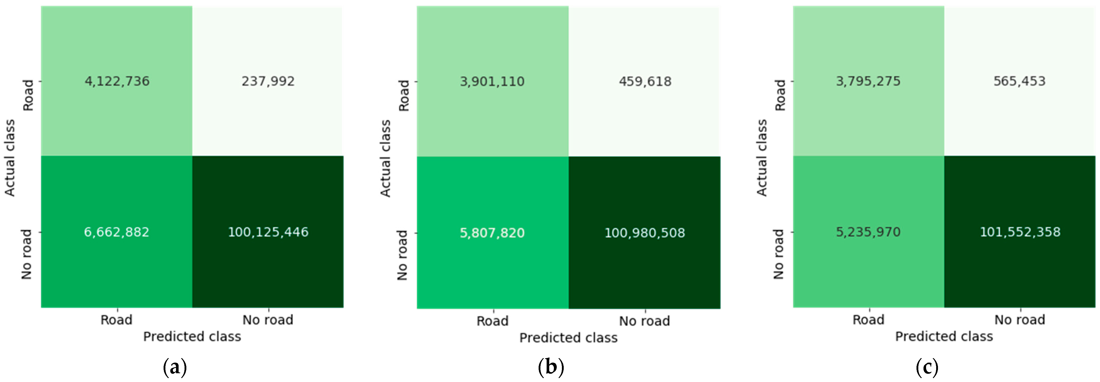
| IoU score | 0.6726 | 0.6741 ± 0.0008 | +0.15% | 0.6750 (+0.24%) | 0.6801 ± 0.0040 | +0.75% | 0.6854 (+1.28%) |
| F1 score (positive class) | 0.5686 | 0.5638 ± 0.0012 | −0.48% | 0.5658 | 0.5714 ± 0.0082 | +0.28% | 0.5819 |
| F1 score (negative class) | 0.9648 | 0.9692 ± 0.0005 | +0.44% | 0.9690 | 0.9711 ± 0.0016 | +0.63% | 0.9729 |
| F1 score | 0.7667 | 0.7665 ± 0.0006 | −0.02% | 0.7674 | 0.7713 ± 0.0040 | +0.46% | 0.7765 |
| Accuracy | 0.9379 | 0.9437 ± 0.0009 | +0.58% | 0.9448 | 0.9475 ± 0.0026 | +0.96% | 0.9503 |
| Precision (positive class) | 0.4183 | 0.4247 ± 0.0019 | +0.64% | 0.4271 | 0.4546 ± 0.0187 | +3.63% | 0.4673 |
| Precision (negative class) | 0.9976 | 0.9953 ± 0.0002 | −0.23% | 0.9953 | 0.9937 ± 0.0014 | −0.39% | 0.9953 |
| Precision | 0.7080 | 0.7100 ± 0.0009 | +0.20% | 0.7112 | 0.7242 ± 0.0089 | +1.62% | 0.7302 |
| Recall (positive class) | 0.9504 | 0.8908 ± 0.0062 | −5.96% | 0.8904 | 0.8376 ± 0.0459 | −11.28% | 0.8947 |
| Recall (negative class) | 0.9372 | 0.9452 ± 0.0012 | +0.80% | 0.9452 | 0.9509 ± 0.0040 | +1.37% | 0.9558 |
| Recall | 0.9438 | 0.9181 ± 0.0025 | −2.57% | 0.9178 | 0.8943 ± 0.0210 | −4.95% | 0.9205 |
Publisher’s Note: MDPI stays neutral with regard to jurisdictional claims in published maps and institutional affiliations. |
© 2022 by the authors. Licensee MDPI, Basel, Switzerland. This article is an open access article distributed under the terms and conditions of the Creative Commons Attribution (CC BY) license (https://creativecommons.org/licenses/by/4.0/).
Share and Cite
Cira, C.-I.; Kada, M.; Manso-Callejo, M.-Á.; Alcarria, R.; Bordel Sanchez, B. Improving Road Surface Area Extraction via Semantic Segmentation with Conditional Generative Learning for Deep Inpainting Operations. ISPRS Int. J. Geo-Inf. 2022, 11, 43. https://doi.org/10.3390/ijgi11010043
Cira C-I, Kada M, Manso-Callejo M-Á, Alcarria R, Bordel Sanchez B. Improving Road Surface Area Extraction via Semantic Segmentation with Conditional Generative Learning for Deep Inpainting Operations. ISPRS International Journal of Geo-Information. 2022; 11(1):43. https://doi.org/10.3390/ijgi11010043
Chicago/Turabian StyleCira, Calimanut-Ionut, Martin Kada, Miguel-Ángel Manso-Callejo, Ramón Alcarria, and Borja Bordel Sanchez. 2022. "Improving Road Surface Area Extraction via Semantic Segmentation with Conditional Generative Learning for Deep Inpainting Operations" ISPRS International Journal of Geo-Information 11, no. 1: 43. https://doi.org/10.3390/ijgi11010043
APA StyleCira, C.-I., Kada, M., Manso-Callejo, M.-Á., Alcarria, R., & Bordel Sanchez, B. (2022). Improving Road Surface Area Extraction via Semantic Segmentation with Conditional Generative Learning for Deep Inpainting Operations. ISPRS International Journal of Geo-Information, 11(1), 43. https://doi.org/10.3390/ijgi11010043