Article

Improving Road Surface Area Extraction via Semantic Segmentation with Conditional Generative Learning for Deep Inpainting Operations

by
Calimanut-Ionut Cira
1,*,
Martin Kada
2,
Miguel-Ángel Manso-Callejo
1,
Ramón Alcarria
1 and
Borja Bordel Sanchez
3
1
Departamento de Ingeniería Topográfica y Cartografía, E.T.S.I. en Topografía, Geodesia y Cartografía, Universidad Politécnica de Madrid, 28031 Madrid, Spain
2
Institut für Geodäsie und Geoinformationstechnik, Technische Universität Berlin, 10553 Berlin, Germany
3
Departamento de Sistemas Informáticos, E.T.S.I. de Sistemas Informáticos, Universidad Politécnica de Madrid, 28031 Madrid, Spain
*
Author to whom correspondence should be addressed.
ISPRS Int. J. Geo-Inf. 2022, 11(1), 43; https://doi.org/10.3390/ijgi11010043
Submission received: 21 October 2021 / Revised: 22 December 2021 / Accepted: 6 January 2022 / Published: 9 January 2022
(This article belongs to the Special Issue Deep Learning and Computer Vision for GeoInformation Sciences)

Abstract

:
The road surface area extraction task is generally carried out via semantic segmentation over remotely-sensed imagery. However, this supervised learning task is often costly as it requires remote sensing images labelled at the pixel level, and the results are not always satisfactory (presence of discontinuities, overlooked connection points, or isolated road segments). On the other hand, unsupervised learning does not require labelled data and can be employed for post-processing the geometries of geospatial objects extracted via semantic segmentation. In this work, we implement a conditional Generative Adversarial Network to reconstruct road geometries via deep inpainting procedures on a new dataset containing unlabelled road samples from challenging areas present in official cartographic support from Spain. The goal is to improve the initial road representations obtained with semantic segmentation models via generative learning. The performance of the model was evaluated on unseen data by conducting a metrical comparison where a maximum Intersection over Union (IoU) score improvement of 1.3% was observed when compared to the initial semantic segmentation result. Next, we evaluated the appropriateness of applying unsupervised generative learning using a qualitative perceptual validation to identify the strengths and weaknesses of the proposed method in very complex scenarios and gain a better intuition of the model’s behaviour when performing large-scale post-processing with generative learning and deep inpainting procedures and observed important improvements in the generated data.

1. Introduction

In one of our previous works [1] related to road extraction using state-of-the-art semantic segmentation models for automatic mapping purposes, we observed the problem of inaccurate extraction of road geometries, even when working with a large-scale dataset containing information from different regions of Spain (built to improve the generalisation capacity of the resulting models). In the study, frequent discontinuities in the extracted segmentation masks (gaps and missing connection points) were observed, resulting in unconnected road segments. The predictions displayed higher rates of False Positives (FP) in areas where surrounding geospatial objects have a similar spectral signature with the roads, and higher rates of False Negatives (FN) in areas where obstructions are present in the scenes. We concluded that these imperfections were caused by the complex nature of the geospatial object (roads have large curvature changes, different materials used in the pavement, different widths, depending on the importance of the route, and very often have no clearly defined borders) by the presence of occlusions in the scenes, and by the limitation of existing semantic segmentation algorithms. These imperfections and errors are in line with issues raised by other investigations, as similar problems were identified in other works tackling the road extraction task from high-resolution remote sensing images [2,3,4,5], and are very problematic when pursuing a large-scale road extraction operation for automatic mapping purposes. As a consequence, we consider that adding a post-processing operation to improve the initial segmentation predictions is essential for a successful road extraction. In this work, the goal of the post-processing operation is to link road segments more fluidly, to infer small missing road segments, and to eliminate isolated road segments (that have no continuity).
As mentioned previously, one of the most common problems encountered was related to the overlook of connection points, resulting in unconnected road segments (an example can be seen in Figure 1). Traditionally, the post-processing operation has been carried out using conditional random fields [6] or shape filtering [7,8]. However, nowadays, approaches based on inpainting operations are more widely used. Inpainting is a popular computer vision operation introduced by Bertalmío et al. in [9] to reconstruct missing image parts and is aimed at recovering deteriorated areas in images. For an initial post-processing test, we developed an inpainting algorithm containing a kernel of size 4 × 4 pixels to apply morphological operations over the initial segmentation maps (processing based on shapes). The algorithm is able to perform an initial suboperation of erosion of the road boundaries to diminish the features and remove noise, followed by a dilation sub-operation to increase the object area and to accentuate features. Using the same kernel, the objects are returned to their original size. These two operations combined achieve an isolation of individual elements and a more efficient joining of slightly separated elements.
However, we believe that in order to successfully tackle a large-scale post-processing of challenging geospatial targets (such as the road network), more complex post-processing implementations based on deep learning (DL) are required. DL models proved to be better suited for data-intensive applications, traditional machine learning (ML) algorithms having a more limited generalisation capability [10]. Pathak et al. [11] were among the first to use unsupervised learning to understand the context of an image and produce plausible pixel predictions for the missing parts. They proposed a model based on generative learning and convolutional neural networks (CNNs) to generate plausible missing image content at the pixel level, conditioned on its surroundings.
In this work, we pose the post-processing operation as a deep inpainting task (given the nature of the imperfections and the errors identified) and propose a conditional Generative Adversarial Network (cGAN) to tackle it. The cGAN training is done via unsupervised generative learning techniques on a novel dataset with the goal of learning the distribution of roads present in official cartography and reducing the effect of the problems encountered over the initial predictions. The performance of the model was evaluated on unseen data, and maximum improvements in the order of 1.3% in terms of Intersection over Union (IoU) score, I o U = T P / ( T P + F P + F N ) , were observed. It is known that the IoU score is very sensitive, especially in remote sensing scenarios where classes tend to be very unbalanced cases (road pixels generally occupy around 10% of the pixels in the image), because it does not consider True Negatives in computing the performance metric, and even small increases can result as significant [12]. For this reason, we also conduct a qualitative evaluation of the results to identify some of the strengths and weaknesses of the proposed method in very complex scenarios and to establish future research directions. To the best of our knowledge, this is the first instance of large-scale road post-processing using such an approach.
The contributions of this paper are summarised as follows:
  • We implemented a cGAN model for the deep inpainting task to improve the initial semantic segmentation predictions of roads. We proposed generator, G , and discriminator, D , architectures in order to make the training better suited for our learning objective. G is a U-Net [13]-like network, heavily modified for computational efficiency, while D is a modified PatchGAN [14], adapted to process images of 256 × 256 pixels.
  • We trained the model on a new dataset composed of n = 6784 real segmentation maps of roads present in official cartography. Here, we applied randomness in the form of synthetic gaps to the input for training G (which will result in many possible corrupted images [15]). This source of randomness applied to the conditional information allows G to generate realistic images. We validated the model on a new test set composed of n = 1696 real semantic segmentation predictions obtained by a state-of-the-art semantic segmentation network (with U-Net as base architecture and SEResNeXt50 [16] as segmentation backbone). We performed this operation at large-scale, with an intent to obtain a production model capable of successfully reducing human participation in the road extraction task.
  • We studied the appropriateness of applying generative learning with inpainting operations for the task of road post-processing by evaluating the model’s ability in generating new samples from the learned domain and conducting metrical comparison and perceptual validation operations. The cGAN proposed achieved a maximum increase of 1.28% over the IoU score obtained by the semantic segmentation model.
We proceed as follows. In Section 2, we discuss works related to road extraction and post-processing. In Section 3, we offer background on conditional Generative Adversarial Networks and their training procedure. The data used in the study is described in Section 4. Details regarding our cGAN implementation are presented in Section 5. The experimental results of the post-processing via deep inpainting are analysed in Section 6 from a quantitative and qualitative perspective. Section 7 presents the conclusions.

2. Related Work

Similarly to Abdollahi et al. [17], we believe that existing work tackling road extraction with DL can be classified based on the type of neural network (NN) applied. First, we have the approaches based on CNNs. Here, the road labels are predicted at a patch level using CNNs, and the final prediction is obtained by assembling the labelled patches. For example, Li et al. [18] proposed a CNN-based approach based on anticipating the possibility of each pixel belonging to a road segment. They also proposed a road centreline extraction technique based on simple image processing with morphological operators and obtained IoU scores of maximum 0.78.
However, the majority of the works related to road extraction with DL techniques follow the semantic segmentation approach, where the fully connected (FC) layers are replaced with interpolation layers that upsample the feature maps from the last layer to the input’s size to predict the labels. Buslaev et al. [19] developed a model following the encoder–decoder structure based on U-Net [13] and ResNet [20] to extract roads from remote sensing imagery and proposed a loss function combining the binary cross-entropy and the Jaccard score to reduce the cost. The model obtained an IoU score of 0.64 on unseen data. Similarly, Xu et al. [21] introduced M-Res-U-Net, a model based on ResNet and U-Net, where a Gaussian filter is applied during pre-processing to reduce the noise in the images. The authors rasterised existing vectoral road cartography data, but the approach underperformed in areas where other geospatial objects had similar colours to the road distribution. Cheng et al. introduced CasNet [22], which includes two cascaded networks—one for detecting road regions and the other for extracting the road centrelines— while taking advantage of the feature maps learned by the first network. The model was trained and tested on a dataset composed of 224 Google Earth images [23] and achieved an IoU score of maximum 0.88. However, the authors recognised the unsuitability of the network for processing areas where tree occlusions are present.
Recently, approaches based on Generative Adversarial Networks (GANs) [24] have emerged. This type of NNs was introduced by Goodfellow et al. in 2014. They are DL generative models based on unsupervised learning (a paradigm of learning where the model is only given the input variables, and no output variables), where two networks (called generator, G , and discriminator, D ) are trained simultaneously in an adversarial setting with the goal of finding the probability function that best describes the training examples. GANs have evolved over the following years [25]. Deep Convolutional GANs (DCGANs) [26] feature deep CNNs in G and D and have proved their usefulness in unsupervised machine vision tasks. The conditional Generative Adversarial Network (cGAN) [27] emerged as an extension that provides both the generator and the discriminator with additional information (for example, using class labels as inputs before applying the noise distribution).
In the field of deep image inpainting, Iizuka et al. proposed GLCIC [28], featuring a global discriminator processing at the image level and a local discriminator processing the centre of the regions to inpaint. In this way, the filled regions achieve a higher global and local consistency. Liu et al. introduced Partial Convolutions (Pconv) [29] (comprising masked and re-normalised convolution operations followed by a mask-update setup) as a method to inpaint multiple irregular holes using deep generative learning and achieved high quality results over irregular masked images. Based on DeepFill v1 [30] (trained to match and combine generated features inside and outside the missing hole), Yu et al. implemented DeepFill v2 [31], featuring Gated Convolution (a Pconv where an extra standard convolutional layer followed by a sigmoid function is added). The model represents the state-of-the-art in the deep image inpainting field.
These advancements allowed the road extraction task to be approached from an unsupervised learning perspective. In [32], de la Fuente Castillo et al. successfully applied unsupervised learning based on grammar-guided genetic programming to obtain new neural network architectures specialised in road recognition in aerial imagery. Varia et al. [33] used the FCN-32 variant [34] and Pix2pix [14] to extract roads from a unmanned aerial vehicle dataset containing 189 training and 23 test images, but observed high rates of FN predictions. Shi et al. [35] developed a cGAN architecture using SegNet [36] (based on the encoder–decoder architecture) as G to segment roads in high-resolution aerial imagery and achieved an F1 score of 0.8831 (3.6% improvement when compared to the F1 score of 0.8472 obtained by SegNet when not trained in an adversarial setting). Yang et al. [37] added the Wasserstein distance penalty to a GAN to achieve an IoU score of 0.73 when extracting road geometries from rural areas in China.
Hartmann et al. [38] trained a GAN architecture to synthetise road information in areas where the extraction is complicated (e.g., where discontinuities are present). Costea et al. [39] proposed a road extraction method composed of an edge detection phase with a GAN, and a later stage of smoothing to post-process the results and improve the initial segmentation predictions. Lastly, Zhang et al. implemented a Multi-conditional GAN (McGAN) [40] to refine the road topology and obtain more complete road network graphs. Different from these works, we wanted to avoid focusing on small, ideal study areas and decided to build a new dataset containing 8480 tiles of 256 × 256 pixels containing roads from official cartography and their correspondent segmentation masks to add real world complexity to the generative task and carry out the experiments on a large scale.
Although there are many works tackling road surface area extraction, post-processing the segmentation predictions is still an active area of research. In [41], we studied the post-processing of semantic segmentation predictions via image-to-image translation operations and proposed a method based on Pix2pix [14], observing impressive results. We believe that another important post-processing application, directly applicable to remote sensing and geospatial element detection, is the inpainting operation, which can be used to reconstruct missing segments by filling in missing parts of the initial semantic segmentation mask. Following this line, Chen et al. [15,42] proposed a method combining adversarial learning with reinforcement learning (a Policy Gradient component [43], where a reinforcement learning approach based on the REINFORCE algorithm [44] is added to a global discriminator) to recover gaps from thin structures in large images, the model proving its performance on reduced datasets containing structures such as retinal vessels, roads, or plant roots. It is worth noting that many models proposed for deep image inpainting follow the multiscale discriminator design, where a global discriminator is used at image level, and a local discriminator is used at the level of the corrupted region.
In this paper, we approach the road post-processing task via generative learning and propose a conditional GAN model to generate improved road semantic segmentation predictions. The model works by corrupting the training images with random holes, and subsequently learning to reconstruct the resulting corrupting images using a cGAN trained for inpainting operations. Finally, the initial segmentation masks, unseen during training, are passed through G to calculate the performance metrics of the model and conduct a perceptual validation of the results.

3. Problem Description

Inpainting [9] is aimed at recovering missing information from images by filling in the deteriorated areas. In this work, we take a model-based approach and train a cGAN using unsupervised learning techniques (where no labelled data is required) for a deep inpainting task. Here, we have a domain, Y , with distribution,   p Y , containing the representations belonging to the official road cartography domain. However, we only have access to a limited number of samples, y n . The goal is that G learns a plausible mapping to Y , given an observation (condition), y , and a random variable, z (resulting a realistic reconstruction, y ˜ = G ( z | y ) ) [45]. Because z   is random, the mapping G learns will come from many possible corrupted images.
G is trained to produce outputs, y ˜ i (belonging to the domain of the reconstructions Y ˜ ), that cannot be distinguished from “real” images, y (belonging to the domain Y ), by an adversarially trained discriminator, D , which is trained to detect the generator’s “fakes”. This way, G will learn to generate synthetic samples,   y ˜ , as close as possible to real samples coming from Y . To avoid saturating gradients early on (when G is not doing well at generating data), instead of taking the traditional approach to minimise the log-probability of G being wrong, m i n   [ 1 l o g ( D ( G ( z | y ) ) ) ] ,   we apply a modified minimax objective,   m i n G m a x D G A N ( G , D ) , and train G to maximise the log-probability of the discriminator D ( y , G ( z | y ) ) being mistaken, l o g ( D ( G ( z | y ) ) . This encourages G to produce samples with a low probability of being “fake”. D is trained via stochastic gradient ascent, m a x   [ l o g   D ( y ) + l o g ( 1 ( D ( G ( z | y ) ) ) ) ] .
The generator network is trained in an unsupervised setting. G   takes a sample, y , from the training data and applies randomness, z , to it (random gaps) to enable the output of many different reconstructed images, instead of only one. By applying the generative function, we obtain a new sample, y ˜ . G is trained so that the fake observation, y ˜ = G ( z | y ) , has a distribution similar to the one of the real observations, y ( p Y ). We also need to take into account that GANs training tends to be unstable and does not always converge as each of the two different players minimises their own cost function [46].

4. Data

In this work, we will use a binarized version of the dataset introduced in [1], obtained from the available openly National Topographical Map, scale 1:50,000 [47], which covers a land area of approximately 181 km2 from representative areas of Spain. This ground truth dataset is based on openly available road data, distributed by a public agency (Geographical National Institute of Spain (Spanish: “Instituto Geográfico Nacional”). According to its producer, the samples were manually tagged by an operator. We divided the dataset containing 8480 tiles with the 80:20% division criteria, resulting in 6784 tiles used for training (80%) and 1696 tiles used for testing (20%) [48]. In this dataset, pixel values of 0 are assigned to pixels belonging to the “No road” class, and pixel values of 1 are assigned to pixels belonging to the “Road exists” class.
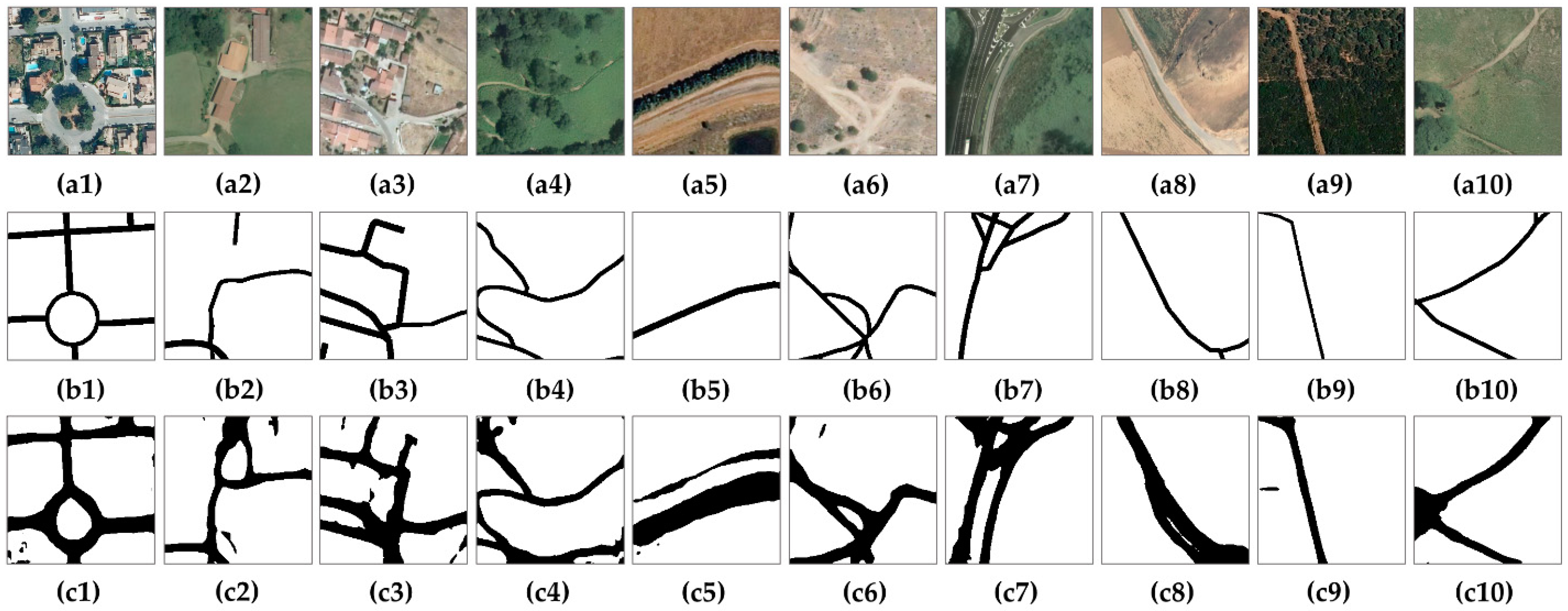
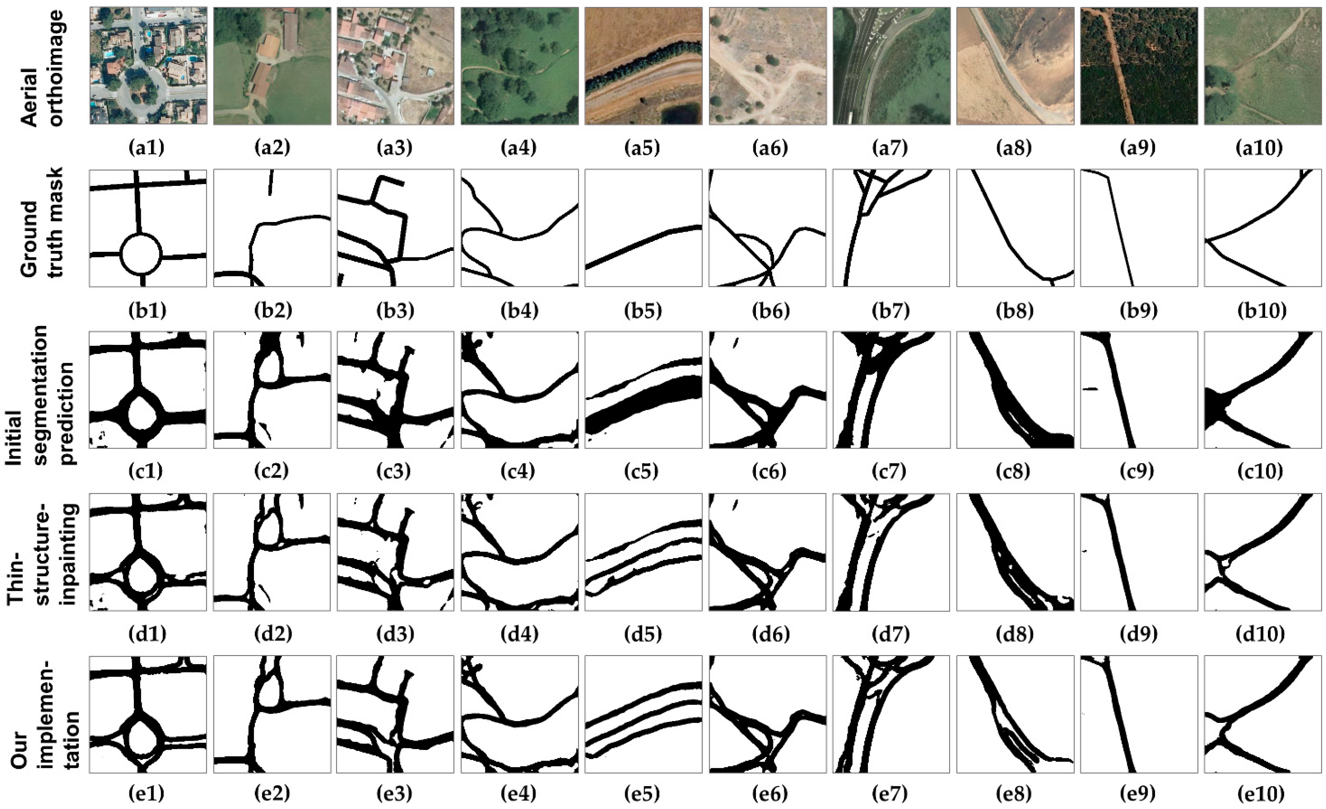
The best-performing semantic segmentation model trained on this dataset obtained a maximum IoU score of 0.6726 on the test set containing unseen data (an IoU score higher than 0.5 is considered a good prediction [49]). This value represents our initial performance value and will be used in the metrical evaluation of the model. Although we do not have any kind of supervision, the segmentation masks obtained from evaluating the test set with the best performing semantic segmentation model (U-Net [13]—SEResNeXt50 [16]) were stored in the lossless PNG (Portable Network Graphics) format and are considered the initial segmentation predictions, being used to assess and study the performance of the proposed cGAN. Please note that only the maximum results delivered are considered (which become our starting point, or base values), as we seek to improve the road extraction via deep inpainting operations. In Figure 2, we can find examples describing the correspondence between the aerial orthoimage, the binarised ground-truth segmentation mask (used for training), and the initial segmentation prediction (used for testing) from ten random tiles.
We want our model to learn the distribution of the roads present in official cartographic support. Therefore, we will use images from the second row as conditional information during training. Afterwards, we will evaluate the initial segmentation masks (third row) using the trained generator to obtain the results of the deep generative inpainting operation. The predictions will be stored to calculate the performance metrics of the proposed model and conduct an exhaustive analysis of the inpainting results delivered.

5. cGAN for Post-Processing Road Predictions via Deep Inpainting Operations

The deep inpainting operation is carried out using a conditional Generative Adversarial Network, where the ground truth label is added as a condition to the input. Generative models are capable of generating new data instances, and the training objective is that G learns how to synthetise data from a distribution, Y (describing the road network present in official cartography), using the training examples, in a way that D is no longer able to distinguish between the data coming from the real road distribution, Y , and the generated data from the synthetic distribution, Y ˜ .   We do that by constraining   y ˜ = G ( z | y ) to be close to y via a defined adversarial loss.

5.1. Generator G

G will take as input tiles of 256 × 256 pixels corrupted with random gaps of different sizes and is trained to correctly reconstruct the corrupted tiles. G does not know the location of the introduced gaps and is forced to learn to automatically detect and inpaint gaps using feedback received from the discriminator network. By applying the generative function, G will output a reconstructed tile, y ˜ = G ( z | y ) . This new sample, G ( z | y ) , should be reasonably similar to the training data distribution, Y .
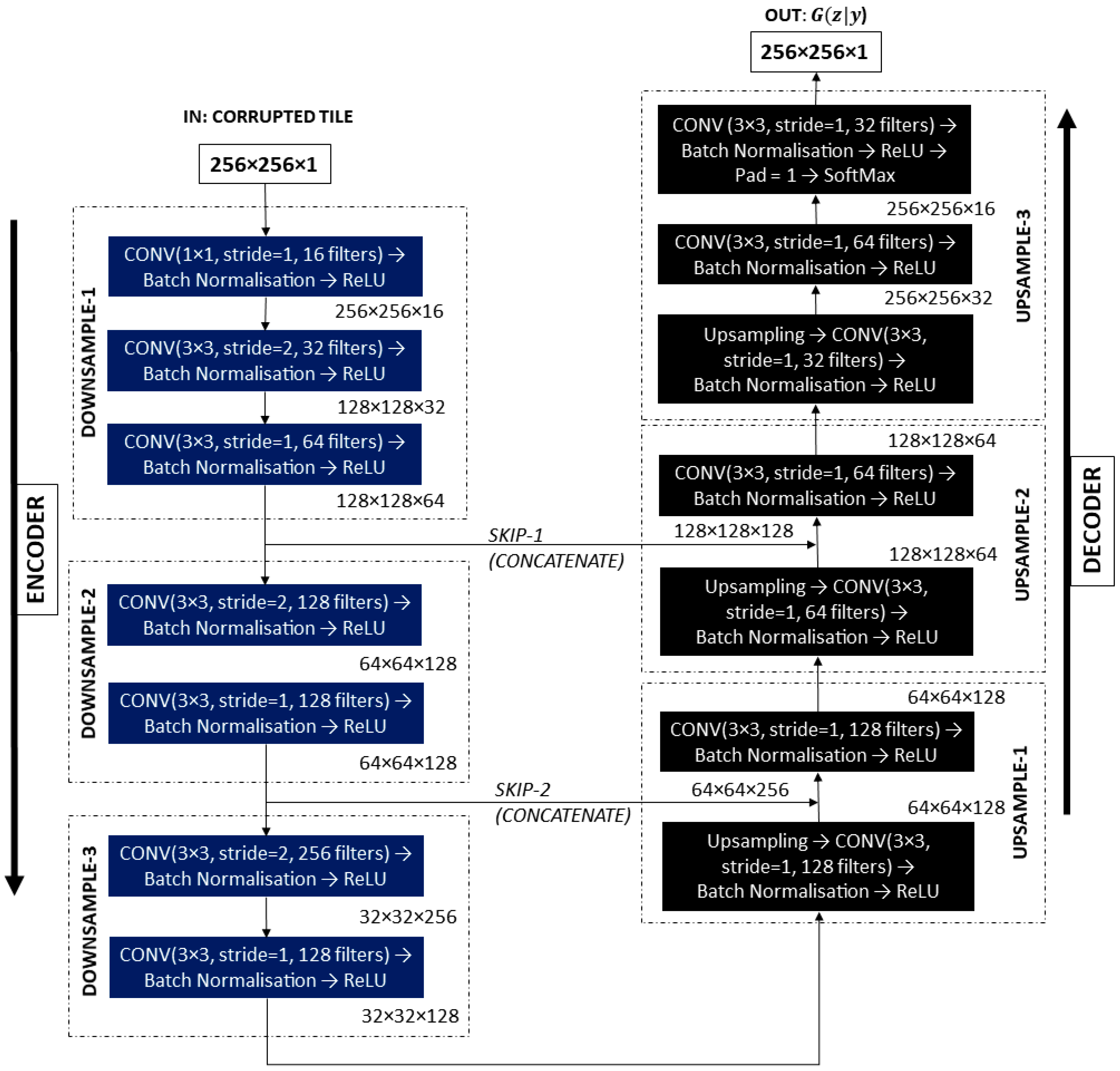
In terms of the architecture, the generator is a U-Net-like network and features a series of convolutional layers with a kernel size of 3 × 3 and zero padding added (to avoid tile shrinking during processing) that progressively downsample the input tile. Following the recommendations from [26], in the downsampling blocks of the encoder, the convolutional layers are followed by Batch Normalisation [50] to ensure faster training and Rectified Linear Unit (ReLU) [51] activations.
In the decoder, the process is reversed, and the representations learned are upsampled to 256 × 256 pixels. The feature maps are expanded to the original size through the use of transposed convolutions (by means of fractional-strided convolutions, instead of pooling layers—following recommendations from [26]). In these upsampling blocks of the decoder, the upconvolutions are followed by convolutional layers (as proposed in [52]), Batch Normalisation, and Leaky ReLU activations [53] (as this activation function proved to help with stabilising the cGAN training [54]).
The information passes through all the layers of the generator network. Similarly to U-Net [13], we added skip connections that enable the sharing of low-level information between the encoder and decoder to preserve the features learned in the first layers and provide a better gradient flow. SoftMax activation is applied to the last layer of G   to keep the argmax for each channel and output a single-channel synthetic tile of 256 × 256 pixels (a probability map). A graphical representation of the proposed generator network is presented in Figure 3.
We also focused on increasing the computational efficiency of our generator network. The G architecture described in Figure 4 features 2,006,974 parameters, a 93.53% decrease when compared to the number of parameters featured by the original U-Net architecture for the same input size (31,031,685 parameters).

5.2. Discriminator D

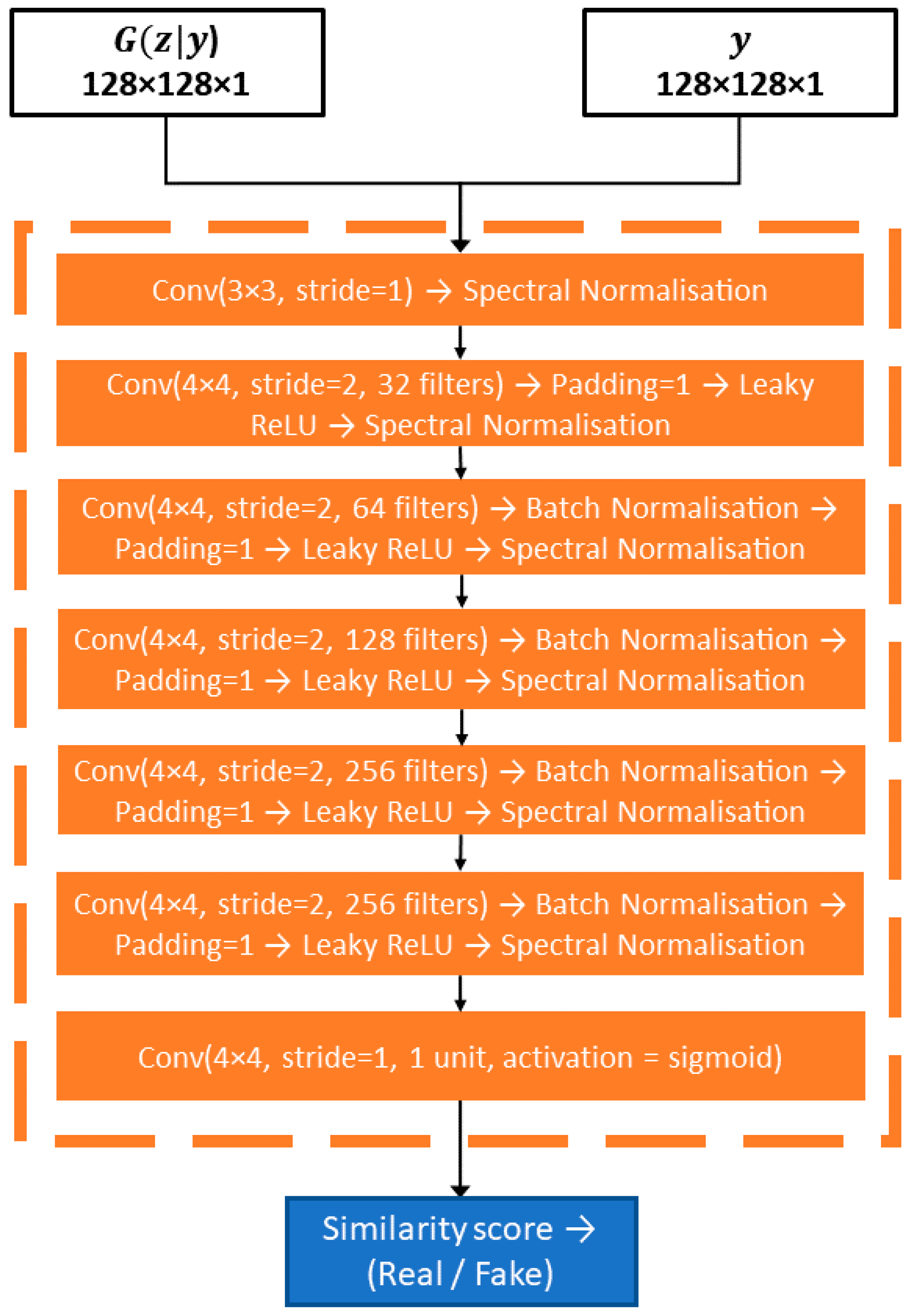
The discriminator network, D , is a modified PatchGAN [14] trained to classify the input tiles and assign the correct distribution of where the input comes from (road distribution present in official cartography, Y , or reconstructed road distribution, Y ˜ ). The input tiles of 256 × 256 pixels in size are divided into four patches of 128 × 128 (instead of 32 × 32, as proposed in the original implementation) to decrease the probability of patches not containing any road element. Each of them is evaluated, and the final decision is the average of the score obtained in each of the four patches (as described in Figure 5 of [41]).
From an architectural viewpoint, D is composed of seven convolutional blocks. The first convolution block features a convolutional layer with a kernel size of 3 × 3 and a stride of 1. We added spectral normalization in each convolutional block to reduce the instability of training the discriminator [55]. The next five convolution blocks consist of convolutional layers with a kernel size of 4 × 4 and a stride of 2, followed by Batch Normalisation. Following the recommendation from [26], we applied Leaky ReLU activation (with a negative slope of 0.2) to all layers from the discriminator and also replaced pooling layers with strided convolutions, as it was proved to ensure a more stable training behaviour [14]. The last block of the discriminator consists of a convolutional layer, with a kernel of 4 × 4 and a stride of 1, ending with a sigmoid activation function that maps the feature maps into a scalar classification score for each patch of 128 × 128 pixels.
A simplified representation of the discriminator network implemented can be found in Figure 4. The total number of parameters of D is 2,791,009, an 85.61% decrease when compared to the original PatchGAN (which features 6,968,257 parameters). Please note that we built our generator and discriminator networks using concepts introduced by U-Net and PatchGAN (e.g., encoder–decoder structures with skip connections, or modelling an image as a Markov random field over a determined patch size), but we focused on reducing the computational footprint of the networks to take advantage of the computational budget available.
The gradient of the output of the discriminator network with respect to the reconstructed data will force G to generate more realistic data (closer to the real data distribution of the road present in the official cartography). In an ideal case, the synthetic data is so close to the real data distribution that D is unable to detect differences between the two data distributions.

5.3. Learning Process

Each input conditional sample, y i , is artificially corrupted by introducing randomness, z , consisting of gaps of different shapes and sizes (square and circular gaps [52], brush gaps [31], and even more unstructured blob gaps [56], or a mix of all of them), as also proposed in [15]. These artificial gaps are randomly rescaled to different sizes, and added online, and represent the source of randomness in the training data that allows G to output many different synthetic outcomes. The gaps are added without a specified location to the conditional data, y ; G ’s training objective is to learn how to inpaint them without knowing their position in the image (the positions of the regions to inpaint are not provided to G ). We also added data augmentation consisting of random 90-degree flips to expose the model to more aspects of the training data and reduce the overfitting behaviour.
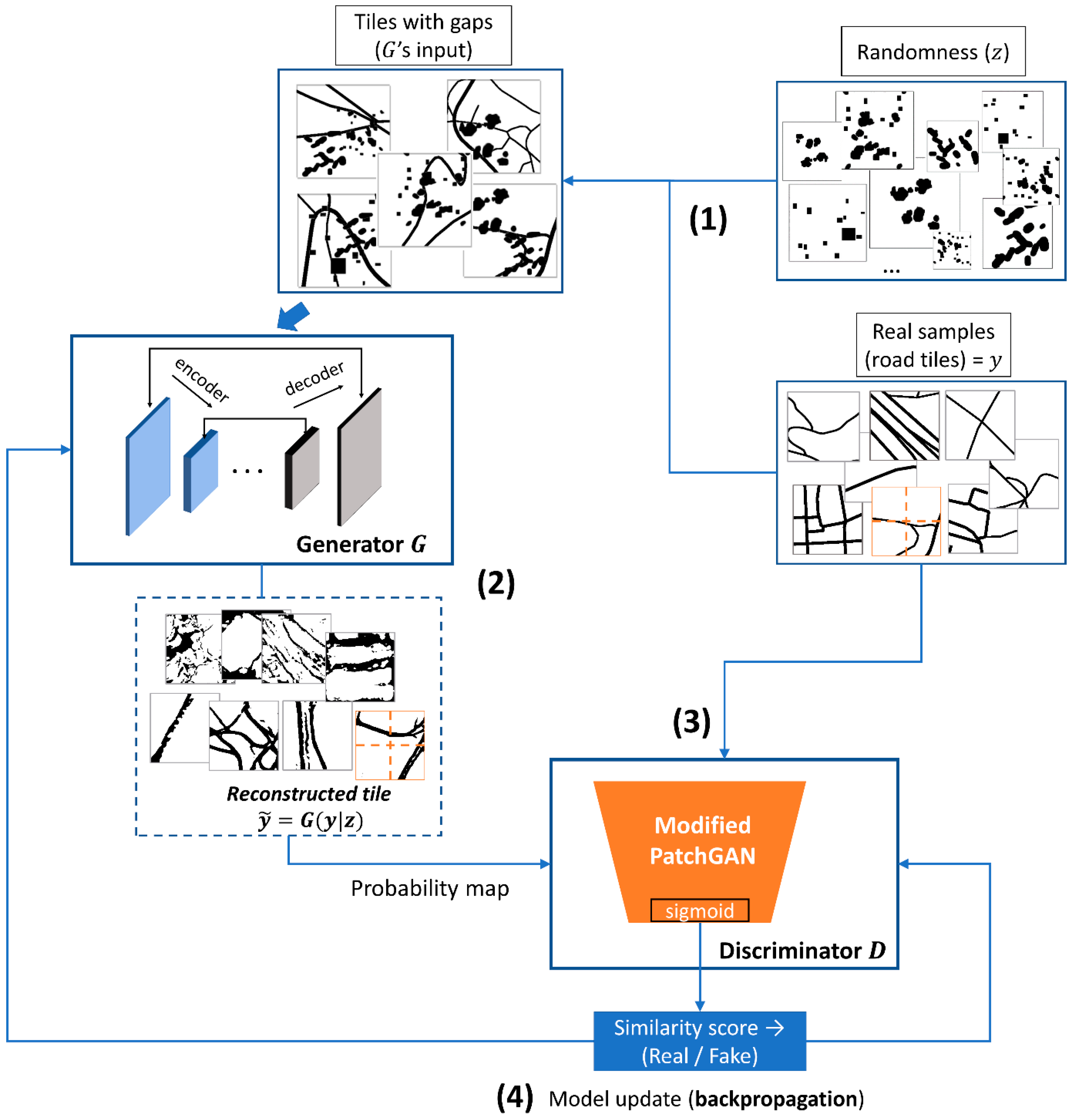
The generator, G , takes a corrupted tile of 256 × 256 pixels as input and provides an inpainted version, where the gaps are filled. Next, D evaluates the four patches of the generated image and the four patches of the original sample from Y (containing a road representation from the official road cartography, without gaps) to calculate the cross entropy between the corresponding pairs of patches of 128 × 128. The error is then backpropagated through the model. A simplified representation describing the learning procedure of the cGAN model implemented can be found in Figure 5.
In Figure 5, it can be seen that the discriminator network is trained with sets of fake and real samples. D tries to identify which images are real ( y ) and which are generated by G ( G ( z | y ) ), while G ’s objective is to generate synthetic tiles that are indistinguishable from the real tiles. The discriminator network takes as input the real sample, y ( D ( y ) to be near 1), and the fake sample, G ( z | y ) , analysing the distribution to decide whether the data is generated or comes from the real sample dataset. D tries to maximise the difference between its output on real tiles and its output on reconstructed tiles (trying to make D ( G ( z | y ) ) near 0, meaning the input is fake), while G tries to make D ( G ( z | y ) ) near 1 (meaning the input is real).
In this case, the discriminator is trained using supervised learning via stochastic gradient ascent with the Least Squares Generative loss (LSGAN) proposed in [57], ( D ) = ( 1 D ( y ) ) 2 + ( D ( G ( z | y ) ) ) 2 . D acts like a binary classifier trained to differentiate between the generated y ˜ = G ( z | y ) [58] and the real sample, y , and features a sigmoid function to assess if the gaps were correctly filled (if the sample is real or not), every input of D having a 0.5 probability of being real and 0.5 of being fake. D   compares each input/target pair at the patch level and estimates the cross entropy between the conditional information, y (before the gaps were introduced), and the reconstructed y ˜ = G ( z | y ) with the formula ( y ^ i ,   y i ) = 1 m i = 1 m y i l o g y ^ i + ( 1 y i ) l o g ( 1 y ^ i ) .   D then provides a probability score at patch level on how realistic they look, averaging the results to provide the overall image mean (used for the model’s loss function). Based on the discriminator’s classification error, the weights are then adjusted to maximise its performance (maximises the probability of D being right) with the following formula: m a x [ l o g   D ( y ) + l o g ( 1 ( D ( G ( z | y ) ) ) ) ] .
The generator network is trained to repair the corrupted tiles, taking a corrupted patch as input, and providing an inpainted version where the random gaps were filled. G predicts a probability map, y ˜ , indicating a pixel’s likelihood to be “Road” or “Background”, and its training objective is to generate synthetic tiles that would be indistinguishable from the real tiles. Unlike D , G does not have access to the real distribution, Y , and uses D ’s gradients to see how realistic the reconstructed tiles are to update its weights. As explained in Section 3, the weights of the generator are adjusted based on the output of the discriminator to maximise the loss predicted by D for generated images marked as “real”; the adversarial cost of G is G = ( 1 D ( G ( z | y ) ) ) 2 . This way, D ’s weights indicating that the generated images were real will force large weight updates in G toward generating more realistic images.
The combined loss function of the model is given by cGAN = λ 1 ( y ^ i ,   y i ) + λ 2 G , where λ 1 = 1000 and λ 2 = 1 . During training, we apply a higher weight to λ 1 for the reconstruction loss to strongly encourage the model towards generating plausible reconstructions of the input image (more realistic images) as it improves the generator’s performance [11]. Over time, G will create more realistic data, while D will become better at differentiating it from the real data distribution, Y [25]. When D cannot determine whether the data comes from the real dataset or the generator (no longer distinguishes real images from fakes), the optimal state is reached.

6. Experiments and Analysis of the Results

We defined the conditional model using the PyTorch v1 [59] deep learning library for Python [60] and trained it on a Ubuntu Linux [61] server with a 20-core Intel Xeon processor and a Nvidia Tesla V100 graphics card with 16 GB of VRAM. We trained the cGAN model with n = 6784 real samples of tiles obtained from official cartographic support where road segments are connected (with a size 256 × 256 pixels, as described in Section 4).
For training G , we used the Adam optimiser [62] with a learning rate of 0.001 and initial decay rates   β 1 = 0.5 and β 1 = 0.999 . The same optimiser was used for D ’s training, but with a learning rate of 0.002 and initial decay rates β 1 = 0.5 and β 1 = 0.999 . We adopted a twice higher learning rate for G to improve the convergence of GANs and different learning rates for G and D to avoid damaging the learned representations [63]. Each training step involves randomly selecting a batch of real samples and generating a batch of synthetic samples based on the real tiles (following the training procedure described in Figure 5). The chosen batch size was 32 images (the maximum allowed by the GPU). During training, the gradient of the loss function with respect to the weights of the network for a single input-output example was backpropagated.
We repeated the experiments five times using random initialization to enable the statistical interpretation of the performance results. Each time, an initial value of 40 epochs was selected, but the loss of the model was monitored, the training stopping when its cost value had not decreased in the previous five epochs. For comparison reasons, we also trained the state-of-the-art, Thin-structure-inpainting model [15] for the same number of repetitions on the same training dataset. We leave for a future study the implementation of a conditional GAN featuring the standard U-Net as generator and the standard PatchGAN as discriminator, due to the significantly higher number of trainable parameters it would feature, and the computational expense required for training such a conditional GAN.
Afterwards, the initial segmentation masks from the test were evaluated with the generators of the trained networks and the predictions were stored in lossless PNG format. The test set contained n = 1696 initial segmentation predictions obtained by U-Net [13]—SEResNeXt50 [16], and achieved an IoU score of 0.6726 (as described in Section 2). The quality of the generated data would prove if the models correctly learned the distribution of the roads present in official cartography and will be used to assess the performance of the networks. Next, the generated data was compared with the ground truth data from the test set (unseen data, to test the generalization capacity of the model) to compute the following performance metrics: IoU score, F1 score, accuracy, and precision and recall, together with the corresponding values calculated for the positive and negative classes. The task of road extraction involves highly unbalanced classes (roads occupy a small portion of an image, generally less than 10%) and the weighted metrics were not computed. The reported results can be found in Table 1.
As shown in Table 1, our implementation outperforms the other methods and obtains the highest performance scores. In relation to the chosen performance metrics, we consider that the IoU score is the most appropriate for evaluating the performance of a model trained for binary operations of geospatial elements (e.g., road and non-road). The reason for this is that classes in such scenarios tend to be very unbalanced (in our dataset, pixels of roads generally occupy around 10% of the pixels), and the traditional ML metrics can mislead regarding the performance of a model [12]. The IoU score is calculated with the formula I o U   s c o r e   ( P , Q ) = | P Q |   | P Q | = | P Q | | P | + | Q | | P Q | , for any two sets, P and Q (e.g., the ground truth set and the reconstructed set generated by G ).
The proposed cGAN model achieved a median IoU score of 0.6801 ± 0.004, which represents an average improvement of 0.75% over the initial semantic segmentation results. The best performing cGAN implementation obtained a maximum IoU score improvement of 1.28% (a performance value of 0.6854, an increase from 0.6726 obtained by U-Net [13]—SEResNeXt50 [16]). When comparing the IoU score results with the ones obtained by Thin-structure-inpainting [15] trained for the same task on the same training set, it can be seen that our implementation outperformed the state-of-the-art model with a maximum difference of 1.04%. Nonetheless, Thin-structure-inpainting [15] also obtained an average IoU score improvement of 0.15% with respect to the initial IoU value obtained by the semantic segmentation model.
Regarding the other performance metrics computed, the precision-recall trade-off scenario [64] is present in both deep inpainting models—both cGAN models trained for deep inpainting operations reduce the FP rates to increase their precision values (a higher precision involves minimising FP rates) at the cost of a decrease in the recall metrics (a higher recall involves minimising FN rates). Our cGAN implementation sacrificed an average of 4.95% from the recall values (which decreased from 0.9438 in the case of the best segmentation model to 0.8943 ± 0.021) to achieve average gains in precision of 1.62% (increases from 0.9379 to 0.9533 ± 0.012) when compared to the original model. This trade-off scenario is to be expected considering that the ground truth dataset contained imbalanced classes with fewer positive samples due to the nature of the studied geospatial object. It is also important to remember that the road representations delivered by the semantic segmentation model had an increased width compared to the considered ground truth (as found in Figure 2b,c), and therefore, the probability of them containing more pixels correctly tagged with the “Road” label in the ground truth (positive samples) was higher. As a result, significant differences can be observed in recall and precision; the deep inpainting models sacrificed recall to increase their precision by increasing the TN and FN ratios. However, precision and recall scores should not be discussed in isolation, and for this reason, the F1 score was also computed. Our implementation achieved a mean increase of +0.46% (0.7713 ± 0.0040) over the initial F1 score value of 0.7667. In Table 1, it can be observed that, although the performance metrics from the positive classes are generally lower, the overall performance scores increased.
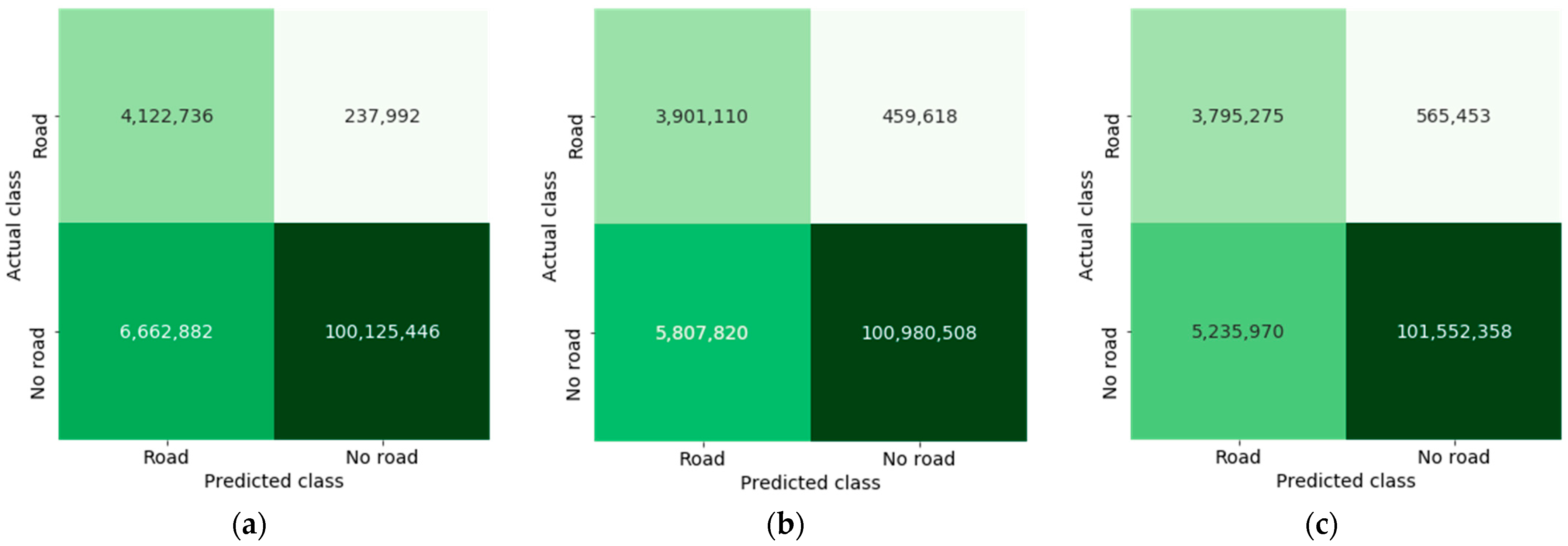
In order to study the relationship between the error rates obtained by the neural networks trained in this work and the significance of the performance metrics, in Figure 6 we illustrate the confusion matrices obtained by the models when evaluating the test set containing unseen data ( n = 1696 tiles). In the confusion matrix obtained by our implementation (presented in Figure 6c), it can be found that our model correctly recognised 3,795,275/4,360,728 pixels belonging to the “Road” class (TP ratio of 0.87) and 101,552,358/106,788,328 “No Road” instances (TN ratio of 0.951), while incorrectly labelling 5,235,970/106,788,328 pixels of the “No Road” category (FP ratio of 0.049) and missing 565,453/4,360,728 instances of the “Road” class (FN ratio of 0.130). In the confusion matrix, FN and FP are the samples that were incorrectly classified and represent 5.22% of the predictions, while TN and TP are the samples that were correctly classified and represent 94.78% of the predictions. By comparison, the segmentation model that provided the initial predictions correctly classified 93.79% of the pixels, while the best version of the Thin-structure [15] model, trained for deep inpainting, correctly classified 94.36% of the pixels. The results from the confusion matrices are aligned with the results presented in Table 1.
It can be observed that, in line with the performance metrics from Table 1, the conditional GANs trained decreased the TP and FP and increased the FN and TN rates in order to optimize their overall performance and inpaint the gaps in the initial road line representations. It can be noted that, although the TP rates are lower compared to the initial segmentation masks, the models significantly improved the TN predictions and increased their mean IoU scores. Overall, the correct predictions have a higher ratio in both deep inpainting scenarios compared to the initial segmentation masks—Thin-structure-inpainting achieved a mean accuracy of 0.9437 ± 0.001, while our implementation achieved a mean accuracy of 0.9475 ± 0.003 and mean improvements of +0.58% and +0.96%, respectively, over the initial accuracy value of 0.9379 obtained by the best performing segmentation model.
In order to obtain a better intuition of what these improvements in performance metrics mean, we conducted a non-numerical qualitative interpretation of the results through means of perceptual validation. We sampled ten images from the test set (containing data unseen by the models during training) and performed a visual inspection of the generated images to compare the results obtained by our implementation and to the ones obtained by the other models. This operation allows us to identify patterns in the studied object that might be impossible to observe with the quantitative methodology (for example, scenarios with higher concentrations of FP and FN). The results are found in Figure 7.
In Figure 7, it can be observed that our implementation generates the most consistent reconstructions, the results delivered being more similar to the ground-truth masks when compared to the initial segmentation masks. We can also identify the reason for the precision-recall trade-off scenario—although the roads representations from official cartography contain no gaps, they do not cover the true road surface area (the lines used to draw the road segments only have cartographic significance and were chosen based on the importance of the road). Although the rates of FP are lower, the models still deliver higher FP rates when compared to the ground truth data because of the representation errors from the available official cartographic support. However, we consider that our conditional implementation correctly learned the road distribution in official cartography, generated less FP rates, and achieved considerable improvements in the results.
We also noted the effect of randomness applied to the conditional data, as our generated data often presented small gap artifacts. However, our real-world dataset contained many more gaps, and the machine predictions obtained with our conditional implementation can be considered significantly improved. In addition, we observed a thinning effect on the post-processed road lines, which helped the networks trained achieve higher performance metrics, as the road representation from official cartography feature an arbitrary-sized width that does not cover the entire surface area of the road.
Although the post-processing results are not perfect, they confirm the appropriateness of applying generative learning for the post-processing task of road semantic segmentation, and we strongly believe that the technique can be applied for a better extraction of geospatial elements from aerial imagery. We consider that the training objective of this study (obtaining road representation closer to the ones present in official cartography) was successfully achieved, as the generated results are clearly representing an improvement over the initial segmentation predictions. The qualitative interpretations carried out proved that the post-processing operation reduced the gaps and the generated predictions that are closer to the target domain (road representations present in official cartography) with the mention that the deep inpainting models are sensitive to the number of holes in the data.

7. Conclusions

To overcome the deficiencies caused by the extraction of roads via semantic segmentation, we implemented a conditional GAN trained to learn the distribution of roads present in official cartography in an unsupervised setting. To the best of our knowledge, this was one of the first attempts for a large-scale post-processing of initial road segmentation with deep inpainting operations based on generative learning to reduce the imperfections found in the initial predictions (e.g., discontinuities and gaps) in an adversarial way.
The proposed cGAN model obtained a maximum improvement of 1.28% in the IoU score on unseen test data when compared to the initial segmentation mask results and outperformed other state-of-the-art models. The qualitative assessment conducted on several scenarios demonstrated the relevance of the reconstruction approach and asserted the performance improvements observed in the metrical comparison—the generated tiles feature road representations that are more similar to the target domain (road distribution present in official cartographic support).
However, as in the case of most deep learning models, the quality of the generated machine predictions was highly dependent on the quality of the conditional training data, and our model is sensitive to the number of holes in the data, the most important source of error being the imperfections present in official cartography. It should be noted that in tasks involving the extraction of unbalanced classes (such as road extraction), even small increments in performance metrics can result as significant, and an additional qualitative evaluation is required on unseen areas.
These results demonstrate the effectiveness of applying conditional generative learning for post-processing image segmentation masks of roads extracted from aerial orthoimages. Although there is room for improvement, our proposal shows the benefit of deep inpainting operations with generative learning as a technique applied to reconstruct gaps in extracted remote sensing objects caused by occlusions in the scenery. The proposed cGAN model is applicable to the binary segmentation results of roads delivered by any segmentation model (where discontinuities are present), and we expect similar improvements over the results.
We believe that, in a world where autonomous vehicles gain in increased importance, the way state administration handles official road cartography must evolve and change from simple road cartographic symbolisation to having complete and openly available road surface area cartography. We plan to keep on improving these road extraction results with other unsupervised approaches, such as image-to-image translation. The end goal is to design an end-to-end solution that can successfully extract roads from extended areas, while correctly preserving the topological properties of the geospatial element.

Author Contributions

Conceptualization, Calimanut-Ionut Cira; data curation, Calimanut-Ionut Cira, Miguel-Ángel Manso-Callejo and Ramón Alcarria; formal analysis, Calimanut-Ionut Cira, Martin Kada, Miguel-Ángel Manso-Callejo, Ramón Alcarria and Borja Bordel Sanchez; funding acquisition, Miguel-Ángel Manso-Callejo and Calimanut-Ionut Cira; investigation, Calimanut-Ionut Cira, Martin Kada, Miguel-Ángel Manso-Callejo, Ramón Alcarria and Borja Bordel Sanchez; methodology, Calimanut-Ionut Cira, Martin Kada, Miguel-Ángel Manso-Callejo, Ramón Alcarria and Borja Bordel Sanchez; project administration, Miguel-Ángel Manso-Callejo; resources, Calimanut-Ionut Cira, Miguel-Ángel Manso-Callejo and Ramón Alcarria; software, Calimanut-Ionut Cira, Martin Kada, Miguel-Ángel Manso-Callejo, Ramón Alcarria; supervision, Martin Kada, Miguel-Ángel Manso-Callejo, Ramón Alcarria and Borja Bordel Sanchez; validation, Calimanut-Ionut Cira, Martin Kada, Miguel-Ángel Manso-Callejo, Ramón Alcarria and Borja Bordel Sanchez; visualization, Calimanut-Ionut Cira, Martin Kada, Miguel-Ángel Manso-Callejo, Ramón Alcarria and Borja Bordel Sanchez; writing–original draft, Calimanut-Ionut Cira; writing–review and editing, Calimanut-Ionut Cira, Martin Kada, Miguel-Ángel Manso-Callejo, Ramón Alcarria and Borja Bordel Sanchez. All authors have read and agreed to the published version of the manuscript.

Funding

This research received funding from the “Deep learning applied to the recognition, semantic segmentation, post-processing and extraction of the geometry of main roads, secondary roads and paths (SROADEX)” project, grant PID2020-116448GB-I00, funded by the AEI, and “Programa Propio de I+D+I 2021” of Universidad Politécnica de Madrid in the form of a research stay of three months grant at Technische Universität Berlin.

Institutional Review Board Statement

Not applicable.

Informed Consent Statement

Not applicable.

Data Availability Statement

The data presented in this study are available on request from the corresponding author. The data are not publicly available due to ongoing efforts to considerably increase the size of the dataset.

Acknowledgments

We thank Mathias Gatti and all other SROADEX participants for their help in the initial phases of the research design, and in generating the dataset.

Conflicts of Interest

The authors declare no conflict of interest. The funders had no role in the design of the study; in the collection, analyses, or interpretation of data; in the writing of the manuscript; or in the decision to publish the results.

References

  1. Cira, C.-I.; Alcarria, R.; Manso-Callejo, M.-Á.; Serradilla, F. A Deep Learning-Based Solution for Large-Scale Extraction of the Secondary Road Network from High-Resolution Aerial Orthoimagery. Appl. Sci. 2020, 10, 7272. [Google Scholar] [CrossRef]
  2. Hu, F.; Xia, G.-S.; Hu, J.; Zhang, L. Transferring Deep Convolutional Neural Networks for the Scene Classification of High-Resolution Remote Sensing Imagery. Remote Sens. 2015, 7, 14680–14707. [Google Scholar] [CrossRef] [Green Version]
  3. Senthilnath, J.; Varia, N.; Dokania, A.; Anand, G.; Benediktsson, J.A. Deep TEC: Deep Transfer Learning with Ensemble Classifier for Road Extraction from UAV Imagery. Remote Sens. 2020, 12, 245. [Google Scholar] [CrossRef] [Green Version]
  4. Shan, B.; Fang, Y. A Cross Entropy Based Deep Neural Network Model for Road Extraction from Satellite Images. Entropy 2020, 22, 535. [Google Scholar] [CrossRef]
  5. Lin, Y.; Xu, D.; Wang, N.; Shi, Z.; Chen, Q. Road Extraction from Very-High-Resolution Remote Sensing Images via a Nested SE-Deeplab Model. Remote Sens. 2020, 12, 2985. [Google Scholar] [CrossRef]
  6. Dong, R.; Li, W.; Fu, H.; Gan, L.; Yu, L.; Zheng, J.; Xia, M. Oil Palm Plantation Mapping from High-Resolution Remote Sensing Images Using Deep Learning. Int. J. Remote Sens. 2020, 41, 2022–2046. [Google Scholar] [CrossRef]
  7. Zhang, Z.; Zhang, X.; Sun, Y.; Zhang, P. Road Centerline Extraction from Very-High-Resolution Aerial Image and LiDAR Data Based on Road Connectivity. Remote Sens. 2018, 10, 1284. [Google Scholar] [CrossRef] [Green Version]
  8. Liu, J.; Qin, Q.; Li, J.; Li, Y. Rural Road Extraction from High-Resolution Remote Sensing Images Based on Geometric Feature Inference. ISPRS Int. J. Geo-Inf. 2017, 6, 314. [Google Scholar] [CrossRef] [Green Version]
  9. Bertalmío, M.; Sapiro, G.; Caselles, V.; Ballester, C. Image Inpainting. In Proceedings of the Proceedings of the 27th Annual Conference on Computer Graphics and Interactive Techniques, SIGGRAPH 2000, New Orleans, LA, USA, 23–28 July 2000; Brown, J.R., Akeley, K., Eds.; ACM: New York, NY, USA, 2000; pp. 417–424. [Google Scholar]
  10. Zhang, C.; Bengio, S.; Hardt, M.; Recht, B.; Vinyals, O. Understanding Deep Learning Requires Rethinking Generalization. In Proceedings of the 5th International Conference on Learning Representations, ICLR 2017, Toulon, France, 24–26 April 2017. Conference Track Proceedings; OpenReview.net, 2017. [Google Scholar]
  11. Pathak, D.; Krähenbühl, P.; Donahue, J.; Darrell, T.; Efros, A.A. Context Encoders: Feature Learning by Inpainting. In Proceedings of the 2016 IEEE Conference on Computer Vision and Pattern Recognition, CVPR 2016, Las Vegas, NV, USA, 27–30 June 2016. [Google Scholar]
  12. Benjdira, B.; Ammar, A.; Koubaa, A.; Ouni, K. Data-Efficient Domain Adaptation for Semantic Segmentation of Aerial Imagery Using Generative Adversarial Networks. Appl. Sci. 2020, 10, 1092. [Google Scholar] [CrossRef] [Green Version]
  13. Ronneberger, O.; Fischer, P.; Brox, T. U-Net: Convolutional Networks for Biomedical Image Segmentation. In Medical Image Computing and Computer-Assisted Intervention—MICCAI 2015; Lecture Notes in Computer Science; Navab, N., Hornegger, J., Wells, W., Frangi, A., Eds.; Springer: Cham, Switzerland, 2015; Volume 9351. [Google Scholar]
  14. Isola, P.; Zhu, J.-Y.; Zhou, T.; Efros, A.A. Image-to-Image Translation with Conditional Adversarial Networks. In Proceedings of the 2017 IEEE Conference on Computer Vision and Pattern Recognition, CVPR 2017, Honolulu, HI, USA, 21–26 July 2017. [Google Scholar]
  15. Chen, H.; Giuffrida, M.V.; Doerner, P.; Tsaftaris, S.A. Blind Inpainting of Large-Scale Masks of Thin Structures with Adversarial and Reinforcement Learning. arXiv 2019, arXiv:1912.02470. [Google Scholar]
  16. Hu, J.; Shen, L.; Sun, G. Squeeze-and-Excitation Networks. In Proceedings of the 2018 IEEE/CVF Conference on Computer Vision and Pattern Recognition, Salt Lake City, UT, USA, 18–23 June 2018; pp. 7132–7141. [Google Scholar]
  17. Abdollahi, A.; Pradhan, B.; Shukla, N.; Chakraborty, S.; Alamri, A. Deep Learning Approaches Applied to Remote Sensing Datasets for Road Extraction: A State-Of-The-Art Review. Remote Sens. 2020, 12, 1444. [Google Scholar] [CrossRef]
  18. Li, P.; Zang, Y.; Wang, C.; Li, J.; Cheng, M.; Luo, L.; Yu, Y. Road Network Extraction via Deep Learning and Line Integral Convolution. In Proceedings of the 2016 IEEE International Geoscience and Remote Sensing Symposium, IGARSS 2016, Beijing, China, 10–15 July 2016. [Google Scholar]
  19. Buslaev, A.; Seferbekov, S.S.; Iglovikov, V.; Shvets, A. Fully Convolutional Network for Automatic Road Extraction From Satellite Imagery. In Proceedings of the 2018 IEEE Conference on Computer Vision and Pattern Recognition Workshops, CVPR Workshops 2018, Salt Lake City, UT, USA, 18–22 June 2018. [Google Scholar]
  20. He, K.; Zhang, X.; Ren, S.; Sun, J. Deep Residual Learning for Image Recognition. In Proceedings of the 2016 IEEE Conference on Computer Vision and Pattern Recognition (CVPR), Las Vegas, NV, USA, 27–30 June 2016; pp. 770–778. [Google Scholar]
  21. Xu, Y.; Feng, Y.; Xie, Z.; Hu, A.; Zhang, X. A Research on Extracting Road Network from High Resolution Remote Sensing Imagery. In Proceedings of the 26th International Conference on Geoinformatics, Geoinformatics 2018, Kunming, China, 28–30 June 2018; Hu, S., Ye, X., Yang, K., Fan, H., Eds.; IEEE: Piscataway, NJ, USA, 2018; pp. 1–4. [Google Scholar]
  22. Cheng, G.; Wang, Y.; Xu, S.; Wang, H.; Xiang, S.; Pan, C. Automatic Road Detection and Centerline Extraction via Cascaded End-to-End Convolutional Neural Network. IEEE Trans. Geosci. Remote. Sens. 2017, 55, 3322–3337. [Google Scholar] [CrossRef]
  23. Wei, Y.; Wang, Z.; Xu, M. Road Structure Refined CNN for Road Extraction in Aerial Image. IEEE Geosci. Remote. Sens. Lett. 2017, 14, 709–713. [Google Scholar] [CrossRef]
  24. Goodfellow, I.J.; Pouget-Abadie, J.; Mirza, M.; Xu, B.; Warde-Farley, D.; Ozair, S.; Courville, A.C.; Bengio, Y. Generative Adversarial Nets. In Proceedings of the Advances in Neural Information Processing Systems 27: Annual Conference on Neural Information Processing Systems 2014, Montreal, QC, Canada, 8–13 December 2014. [Google Scholar]
  25. Pan, Z.; Yu, W.; Yi, X.; Khan, A.; Yuan, F.; Zheng, Y. Recent Progress on Generative Adversarial Networks (GANs): A Survey. IEEE Access 2019, 7, 36322–36333. [Google Scholar] [CrossRef]
  26. Radford, A.; Metz, L.; Chintala, S. Unsupervised Representation Learning with Deep Convolutional Generative Adversarial Networks. In Proceedings of the 4th International Conference on Learning Representations, ICLR 2016, San Juan, Puerto Rico, 2–4 May 2016. [Google Scholar]
  27. Mirza, M.; Osindero, S. Conditional Generative Adversarial Nets. arXiv 2014, arXiv:1411.1784. [Google Scholar]
  28. Iizuka, S.; Simo-Serra, E.; Ishikawa, H. Globally and Locally Consistent Image Completion. ACM Trans. Graph. 2017, 36, 107:1–107:14. [Google Scholar] [CrossRef]
  29. Liu, G.; Reda, F.A.; Shih, K.J.; Wang, T.-C.; Tao, A.; Catanzaro, B. Image Inpainting for Irregular Holes Using Partial Convolutions. In Proceedings of the Computer Vision—ECCV 2018—15th European Conference, Munich, Germany, 8–14 September 2018. [Google Scholar]
  30. Yu, J.; Lin, Z.; Yang, J.; Shen, X.; Lu, X.; Huang, T.S. Generative Image Inpainting With Contextual Attention. In Proceedings of the 2018 IEEE Conference on Computer Vision and Pattern Recognition, CVPR 2018, Salt Lake City, UT, USA, 18–22 June 2018. [Google Scholar]
  31. Yu, J.; Lin, Z.; Yang, J.; Shen, X.; Lu, X.; Huang, T.S. Free-Form Image Inpainting With Gated Convolution. In Proceedings of the 2019 IEEE/CVF International Conference on Computer Vision, ICCV 2019, Seoul, Korea, 27 October–2 November 2019. [Google Scholar]
  32. de la Fuente Castillo, V.; Díaz-Álvarez, A.; Manso-Callejo, M.-Á.; Serradilla García, F. Grammar Guided Genetic Programming for Network Architecture Search and Road Detection on Aerial Orthophotography. Appl. Sci. 2020, 10, 3953. [Google Scholar] [CrossRef]
  33. Varia, N.; Dokania, A.; Jayavelu, S. DeepExt: A Convolution Neural Network for Road Extraction Using RGB Images Captured by UAV. In Proceedings of the IEEE Symposium Series on Computational Intelligence, SSCI 2018, Bangalore, India, 18–21 November 2018. [Google Scholar]
  34. Long, J.; Shelhamer, E.; Darrell, T. Fully Convolutional Networks for Semantic Segmentation. In Proceedings of the 2015 IEEE Conference on Computer Vision and Pattern Recognition (CVPR), Boston, MA, USA, 7–12 June 2015. [Google Scholar]
  35. Shi, Q.; Liu, X.; Li, X. Road Detection From Remote Sensing Images by Generative Adversarial Networks. IEEE Access 2018, 6, 25486–25494. [Google Scholar] [CrossRef]
  36. Badrinarayanan, V.; Kendall, A.; Cipolla, R. SegNet: A Deep Convolutional Encoder-Decoder Architecture for Image Segmentation. IEEE Trans. Pattern Anal. Mach. Intell. 2017, 39, 2481–2495. [Google Scholar] [CrossRef] [PubMed]
  37. Yang, C.; Wang, Z. An Ensemble Wasserstein Generative Adversarial Network Method for Road Extraction from High Resolution Remote Sensing Images in Rural Areas. IEEE Access 2020, 8, 174317–174324. [Google Scholar] [CrossRef]
  38. Hartmann, S.; Weinmann, M.; Wessel, R.; Klein, R. StreetGAN: Towards Road Network Synthesis with Generative Adversarial Networks. In Proceedings of the International Conference on Computer Graphics, Visualization and Computer Vision Co-Operation with EUROGRAPHICS Association, Plzen, Czech Republic, 29 May–2 June 2017. [Google Scholar]
  39. Costea, D.; Marcu, A.; Leordeanu, M.; Slusanschi, E. Creating Roadmaps in Aerial Images with Generative Adversarial Networks and Smoothing-Based Optimization. In Proceedings of the 2017 IEEE International Conference on Computer Vision Workshops (ICCVW), Venice, Italy, 22–29 October 2017. [Google Scholar]
  40. Zhang, Y.; Li, X.; Zhang, Q. Road Topology Refinement via a Multi-Conditional Generative Adversarial Network. Sensors 2019, 19, 1162. [Google Scholar] [CrossRef] [PubMed] [Green Version]
  41. Cira, C.-I.; Manso-Callejo, M.-Á.; Alcarria, R.; Fernández Pareja, T.; Bordel Sánchez, B.; Serradilla, F. Generative Learning for Postprocessing Semantic Segmentation Predictions: A Lightweight Conditional Generative Adversarial Network Based on Pix2pix to Improve the Extraction of Road Surface Areas. Land 2021, 10, 79. [Google Scholar] [CrossRef]
  42. Chen, H.; Valerio Giuffrida, M.; Doerner, P.; Tsaftaris, S.A. Adversarial Large-Scale Root Gap Inpainting. In Proceedings of the IEEE/CVF Conference on Computer Vision and Pattern Recognition (CVPR) Workshops, Long Beach, CA, USA, 16–21 June 2019. [Google Scholar]
  43. Sutton, R.S.; McAllester, D.A.; Singh, S.P.; Mansour, Y. Policy Gradient Methods for Reinforcement Learning with Function Approximation. In Proceedings of the Advances in Neural Information Processing Systems 12, NIPS Conference, Denver, CO, USA, 29 November–4 December 1999. [Google Scholar]
  44. Williams, R.J. Simple Statistical Gradient-Following Algorithms for Connectionist Reinforcement Learning. Mach. Learn. 1992, 8, 229–256. [Google Scholar] [CrossRef] [Green Version]
  45. Pajot, A.; de Bézenac, E.; Gallinari, P. Unsupervised Adversarial Image Inpainting. arXiv 2019, arXiv:1912.12164. [Google Scholar]
  46. Kodali, N.; Abernethy, J.; Hays, J.; Kira, Z. On Convergence and Stability of GANs. arXiv 2017, arXiv:1705.07215. [Google Scholar]
  47. Instituto Geográfico Nacional Centro de Descargas del CNIG (IGN). Available online: http://centrodedescargas.cnig.es (accessed on 3 February 2020).
  48. Cira, C.-I.; Alcarria, R.; Manso-Callejo, M.-Á.; Serradilla, F. A Framework Based on Nesting of Convolutional Neural Networks to Classify Secondary Roads in High Resolution Aerial Orthoimages. Remote Sens. 2020, 12, 765. [Google Scholar] [CrossRef] [Green Version]
  49. Forczmański, P. Performance Evaluation of Selected Thermal Imaging-Based Human Face Detectors. In Proceedings of the 10th International Conference on Computer Recognition Systems CORES 2017, Polanica Zdroj, Poland, 22–24 May 2017. [Google Scholar]
  50. Ioffe, S.; Szegedy, C. Batch Normalization: Accelerating Deep Network Training by Reducing Internal Covariate Shift. In Proceedings of the 32nd International Conference on Machine Learning, Lille, France, 6–11 July 2015; Volume 37, pp. 448–456. [Google Scholar]
  51. Nair, V.; Hinton, G.E. Rectified Linear Units Improve Restricted Boltzmann Machines. In Proceedings of the 27th International Conference on Machine Learning (ICML-10), Haifa, Israel, 21–24 June 2010; Fürnkranz, J., Joachims, T., Eds.; Omnipress: Madison, WI, USA, 2010; pp. 807–814. [Google Scholar]
  52. Sasaki, K.; Iizuka, S.; Simo-Serra, E.; Ishikawa, H. Joint Gap Detection and Inpainting of Line Drawings. In Proceedings of the 2017 IEEE Conference on Computer Vision and Pattern Recognition, CVPR 2017, Honolulu, HI, USA, 21–26 July 2017. [Google Scholar]
  53. Maas, A.L.; Hannun, A.Y.; Ng, A.Y. Rectifier Nonlinearities Improve Neural Network Acoustic Models. In Proceedings of the International Conference on Machine Learning (ICML), Atlanta, GA, USA, 16–21 June 2013. [Google Scholar]
  54. Gulrajani, I.; Ahmed, F.; Arjovsky, M.; Dumoulin, V.; Courville, A.C. Improved Training of Wasserstein GANs. In Proceedings of the Advances in Neural Information Processing Systems 30: Annual Conference on Neural Information Processing Systems 2017, Long Beach, CA, USA, 4–9 December 2017. [Google Scholar]
  55. Miyato, T.; Kataoka, T.; Koyama, M.; Yoshida, Y. Spectral Normalization for Generative Adversarial Networks. In Proceedings of the 6th International Conference on Learning Representations, ICLR 2018, Vancouver, BC, Canada, 30 April–3 May 2018. [Google Scholar]
  56. Dupont, E.; Suresha, S. Probabilistic Semantic Inpainting with Pixel Constrained CNNs. In Proceedings of the 22nd International Conference on Artificial Intelligence and Statistics, AISTATS 2019, Naha, Japan, 16–18 April 2019. [Google Scholar]
  57. Mao, X.; Li, Q.; Xie, H.; Lau, R.Y.K.; Wang, Z.; Smolley, S.P. Least Squares Generative Adversarial Networks. In Proceedings of the IEEE International Conference on Computer Vision, ICCV 2017, Venice, Italy, 22–29 October 2017. [Google Scholar]
  58. Köhler, R.; Schuler, C.J.; Schölkopf, B.; Harmeling, S. Mask-Specific Inpainting with Deep Neural Networks. In Proceedings of the Pattern Recognition—36th German Conference, GCPR 2014, Münster, Germany, 2–5 September 2014. [Google Scholar]
  59. Paszke, A.; Gross, S.; Massa, F.; Lerer, A.; Bradbury, J.; Chanan, G.; Killeen, T.; Lin, Z.; Gimelshein, N.; Antiga, L.; et al. PyTorch: An Imperative Style, High-Performance Deep Learning Library. In Advances in Neural Information Processing Systems 32; Wallach, H., Larochelle, H., Beygelzimer, A., Alché-Buc, F., de Fox, E., Garnett, R., Eds.; Curran Associates, Inc.: Red Hook, NY, USA, 2019; pp. 8024–8035. [Google Scholar]
  60. Van Rossum, G.; Drake, F.L. Python 3 Reference Manual; CreateSpace: Scotts Valley, CA, USA, 2009; ISBN 1-4414-1269-7. [Google Scholar]
  61. Sobell, M.G. A Practical Guide to Ubuntu Linux; Pearson Education: London, UK, 2015. [Google Scholar]
  62. Kingma, D.P.; Ba, J. Adam: A Method for Stochastic Optimization. In Proceedings of the 3rd International Conference on Learning Representations, ICLR 2015, Conference Track Proceedings, San Diego, CA, USA, 7–9 May 2015. [Google Scholar]
  63. Heusel, M.; Ramsauer, H.; Unterthiner, T.; Nessler, B.; Hochreiter, S. GANs Trained by a Two Time-Scale Update Rule Converge to a Local Nash Equilibrium. In Proceedings of the Advances in Neural Information Processing Systems, Long Beach, CA, USA, 4–9 December 2017. [Google Scholar]
  64. Powers, D.M.W. Visualization of Tradeoff in Evaluation: From Precision-Recall & PN to LIFT, ROC & BIRD. arXiv 2015, arXiv:1505.00401. [Google Scholar]
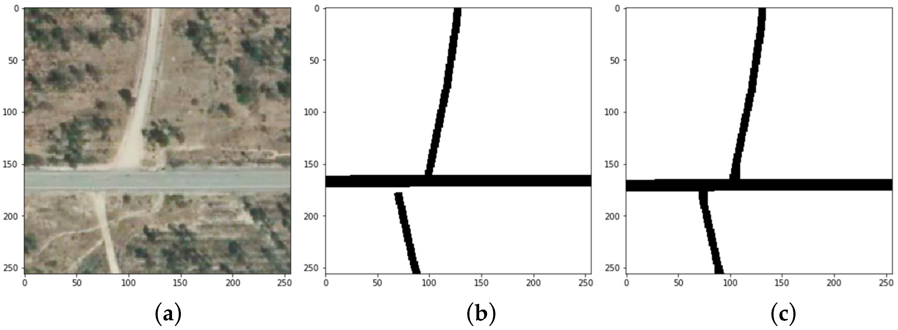
Figure 1. An example of inpainting post-processing with morphology operators based on shapes to fill missing parts (c) of the initial segmentation mask predictions (b) delivered by the semantic segmentation model after evaluating an unseen aerial orthoimage (a).
Ijgi 11 00043 g001
Figure 2. The relation between the aerial orthoimage (first row, (a1a10)), the rasterised segmentation mask (ground-truth or real sample, seen in the second row, (b1b10) used as conditional information for training G ), and the semantic segmentation predictions (seen in the third row, (c1c10), used for testing the performance of the model). Note: The training set contains n = 6784 tiles with road representation present in official cartography, while the test set contains n = 1696 tiles with initial segmentation predictions resulted from evaluating the aerial images with the segmentation model. In this figure, white is used to represent pixels labelled with “No road”, or “Background”, and black is used to represent the pixels belonging to “Road” class.
Ijgi 11 00043 g002
Figure 3. The generator architecture proposed for the deep inpainting operation.
Ijgi 11 00043 g003
Figure 4. The discriminator architecture proposed for the deep inpainting task.
Ijgi 11 00043 g004
Figure 5. An overview of the learning process of the cGAN model trained for deep inpainting. (1) Firstly, random gaps are introduced into the conditional data, y , to produce corrupted inputs for G . (2) The generator (a U-Net-like network with skip connections) is then trained to fill the gaps and inpaint the corrupted tiles. ( G does not have access to the real samples, y , from the real data distribution, Y .) (3) The discriminator is a modified PatchGAN that classifies patches from pairs of y and y ˜ and decides whether they come from the real data distribution, Y , or from the synthetic data distribution, Y ˜ . (4) G receives feedback from D and iteratively improves the synthetic data generator to “fool” the discriminator network. Notes: (A) The real data is fed both into G (after adding z) and into D . In our deep inpainting task, a sampled image, y , will be corrupted with randomness, z (in this case, random gaps of different sizes). G   will reconstruct this corrupted image and produce y ˜ = G ( z | y ) . The synthetic results, y ˜ ,   will iteratively improve as G receives feedback from D . (B) The graphic should be interpreted at stage level and was created using random tiles to offer insights and enable a better understanding of the training procedure presented in Section 5.3.
Ijgi 11 00043 g005
Figure 6. The confusion matrices obtained by (a) the semantic segmentation model U-Net [13]—SEResNeXt50 [16], and (b) Thin-structure-inpainting [15], together with (c) our implementation proposed in Section 5 (trained for deep inpainting operations) on the test set ( n = 1696 tiles).
Ijgi 11 00043 g006
Figure 7. Qualitative interpretation carried out on ten samples from the test set. In the first row (a1a10), we have the aerial orthoimage. The second row (b1b10) presents the samples from the rasterised ground truth set, or conditional data distribution (road representations present in official cartography). The third row (c1c10) shows the initial segmentation prediction obtained using a state-of-the-art semantic segmentation model. The fourth row (d1d10) presents the predictions generated with the Thin-Structure-Inpainting model [15] trained for deep inpainting operations, while the fifth row (e1e10) presents the reconstructed road masks generated with the conditional generative model proposed in this paper.
Ijgi 11 00043 g007
Table 1. Comparison between the performance metrics obtained by the best performing semantic segmentation model trained for road extraction, and the original Thin-structure-inpainting model [15] and our cGAN implementation trained for deep inpainting operations on the test set containing unseen data ( n = 1696 tiles).
Performance Metric(1) Best Performing Semantic Segmentation Model(2) Thin-Structure-Inpainting [15](3) Our cGAN Implementation
Average Result and Standard DeviationMean Percentage Difference (Initial Segmentation Results)Maximum ResultAverage Result and Standard DeviationMean Percentage Difference (Initial Segmentation Results)Maximum Result
IoU score (positive class)0.41000.4068 ± 0.0012−0.32%0.40880.4149 ± 0.0073+0.49%0.4252
IoU score (negative class)0.93520.9414 ± 0.0009+0.61%0.94120.9454 ± 0.0028+1.02%0.9484
IoU score0.67260.6741 ± 0.0008+0.15%0.6750
(+0.24%)
0.6801 ± 0.0040+0.75%0.6854
(+1.28%)
F1 score (positive class)0.56860.5638 ± 0.0012−0.48%0.56580.5714 ± 0.0082+0.28%0.5819
F1 score (negative class)0.96480.9692 ± 0.0005+0.44%0.96900.9711 ± 0.0016+0.63%0.9729
F1 score0.76670.7665 ± 0.0006−0.02%0.76740.7713 ± 0.0040+0.46%0.7765
Accuracy0.93790.9437 ± 0.0009+0.58%0.94480.9475 ± 0.0026+0.96%0.9503
Precision (positive class)0.41830.4247 ± 0.0019+0.64%0.42710.4546 ± 0.0187+3.63%0.4673
Precision (negative class)0.99760.9953 ± 0.0002−0.23%0.99530.9937 ± 0.0014−0.39%0.9953
Precision0.70800.7100 ± 0.0009+0.20%0.71120.7242 ± 0.0089+1.62%0.7302
Recall (positive class)0.95040.8908 ± 0.0062−5.96%0.89040.8376 ± 0.0459−11.28%0.8947
Recall (negative class)0.93720.9452 ± 0.0012+0.80%0.94520.9509 ± 0.0040+1.37%0.9558
Recall0.94380.9181 ± 0.0025−2.57%0.91780.8943 ± 0.0210−4.95%0.9205
Publisher’s Note: MDPI stays neutral with regard to jurisdictional claims in published maps and institutional affiliations.