
Machine Learning of Spatial Data


1
Infrastructure and Environmental Systems Program, University of North Carolina at Charlotte, 9201 University City Blvd., Charlotte, NC 28223, USA
2
Department of Geography and Earth Sciences, University of North Carolina at Charlotte, 9201 University City Blvd., Charlotte, NC 28223, USA
3
School of Data Science, University of North Carolina at Charlotte, 9201 University City Blvd., Charlotte, NC 28223, USA
*
Author to whom correspondence should be addressed.
†
These authors contributed equally to this work.
ISPRS Int. J. Geo-Inf. 2021, 10(9), 600; https://doi.org/10.3390/ijgi10090600
Submission received: 27 July 2021
/
Revised: 8 September 2021
/
Accepted: 9 September 2021
/
Published: 12 September 2021
Abstract
:Properties of spatially explicit data are often ignored or inadequately handled in machine learning for spatial domains of application. At the same time, resources that would identify these properties and investigate their influence and methods to handle them in machine learning applications are lagging behind. In this survey of the literature, we seek to identify and discuss spatial properties of data that influence the performance of machine learning. We review some of the best practices in handling such properties in spatial domains and discuss their advantages and disadvantages. We recognize two broad strands in this literature. In the first, the properties of spatial data are developed in the spatial observation matrix without amending the substance of the learning algorithm; in the other, spatial data properties are handled in the learning algorithm itself. While the latter have been far less explored, we argue that they offer the most promising prospects for the future of spatial machine learning.
1. Introduction
Machine learning (ML) has become a widely used approach in almost every discipline to solve a broad range of tasks and problems with structured and unstructured data, including but not limited to regression, grouping, classification, and prediction. It has proved itself to be a powerful and effective tool in various disciplinary fields and domains of application where spatial aspects are essential, including the following: land use and land cover classification [1,2], cross-sectional characterization [3,4] and longitudinal change [5], urban growth [6] and gentrification [7], disaster management [8], agriculture and crop yield prediction [9], infectious disease emergence and spread [10], transportation and crash analysis [11], map visualization and cartography [12,13], delineation of geographic regions [14] and habitat mapping [15], geographic information retrieval and text matching [16], POI and region recommendation [17], trajectory and movement pattern prediction [18], point cloud classification [19], spatial interaction [20], spatial interpolation [21], and spatiotemporal prediction [22,23,24].
Spatial data exhibit certain distinctive properties that set them apart from other data types, such as spatial dependence, spatial heterogeneity, and scale. As in other modeling approaches, we need to be aware of the specificities that these properties entail when we conduct ML on spatial data. Indeed, the explicit handling of these spatial properties can improve the performance of the ML model or add meaningful insights into the process of learning a task. At the same time, failure to appropriately include these properties into the ML model can negatively impact learning [11,21,22,23,24,25,26].
Surveys of the extant literature have previously been conducted on several themes intersecting with spatial ML, namely knowledge discovery and data mining [27,28,29], spatial prediction methods [30], artificial neural networks in geospatial analysis [31], ML for spatial environmental data [25], and active deep learning for geo-text and image classification [32]. While their contribution to furthering scholarship in spatial ML is unquestionable, these surveys are rather limited in scope. For instance, while there are overlaps between data mining and ML, they have distinct definitions, follow different processes, and have different goals. The emphasis of other literature surveys is on a specific discipline or learning method. In addition, the focus has usually been on applications; a detailed discussion of spatial properties and their role in the ML process is still missing. At this juncture, there is extensive literature that applies ML to spatial data but research that explicitly features the spatial properties of data in ML remains rather limited. Thus, this paper aims to review some of the best recent practices with ML of spatial data while considering the learning process and the properties of spatial data for the purpose of full understanding:
- How much progress in handling spatial properties of data in ML has been accomplished?
- What are some of the best practices in this respect?
- What are the gaps that may remain in this literature, and where do opportunities exist for future research with, and on, spatially explicit ML?
Figure 1a shows our review framework. An initial bibliography search (search strategy 1) through article titles, review papers, and book chapters for exact combination of keywords ‘spatial heterogeneity’, ‘spatial dependence’, ‘scale’, ‘machine learning’, ‘neural network’, and ‘deep learning’ in the Web of Science abstract and citation database resulted in 923 records after filtering out duplicates. Analysis of the records indicated that, while significant attention has been directed toward the machine learning of spatial data in the past few years (Figure 1b), not much attention has so far explicitly been devoted to the fundamental properties of spatial data (Figure 1c). Based on this observation, most of the previous literature that apply ML for spatial data either ignores spatial properties of data or addresses them marginally in their research study. Given the focused objective and the research questions of this paper, and the fact that spatial properties have usually been addressed marginally in the literature, a systematic review with keywords may not be the best way to search through the literature. Thus, we conduct a more focused literature search mainly in journals related to spatial science. This second strategy is useful to reduce the search space to find papers that go beyond application and aim to address properties related to spatial data even marginally as a part of their research questions. Thus, we design a repetitive search process in high quality journals, including but not limited to the International Journal of Geographical Information Science (IJGIS), Transactions in GIS, GIScience & Remote Sensing, Computers, Environment and Urban Systems, Journal of Spatial Science, Remote Sensing of Environment, ISPRS International Journal of Geo-Information, Cartography and Geographic Information Science, Remote Sensing, and ISPRS Journal of Photogrammetry and Remote Sensing. We initially search combinations of keywords ‘machine learning’, ‘deep learning’, ‘heterogeneity’, ‘spatial dependence’, and ‘scale’ to extract papers. Then, we go through their abstracts to see if they have accounted for properties of spatial data, and extract those with direct relation to the objective of this paper. We scan through these papers. If a new challenge is raised in a paper, the related keywords are extracted, and a supplementary search in the journals or in Google Scholar is conducted to find related literature. This process is repeated until the topic is sufficiently discussed. Otherwise, we consider it to be an existing gap in the literature. Within the final database, we divide the related literature into two main categories. The first category includes processes that handle spatial data within the spatial observation matrix. The second category handles spatial properties of data in the learning process instead. Depending on the target application and problem, one may employ one or multiple approaches that are presented to account for spatial properties of data. Interested readers can explore more deeply the topics broached in this paper by following some of the references provided herein. Furthermore, it is not our intention to provide a general comparison between ML methods. For such a purpose, interested readers are referred to [5].
The rest of this paper is organized as follows. We begin with a brief overview of ML (Section 2) and of spatial properties of data (Section 3). Then, we lay out the process of ML of spatial data (Section 4) in two steps, entailing the construction of a spatial observation matrix (Section 4.1) and a learning algorithm (Section 4.2). Section 5 is concerned with the ML of spatiotemporal data. Section 4 and Section 5 serve to answer the first two questions that are the core of this review paper. Finally, we summarize the review work conducted for this paper, discuss the gaps in the current state of knowledge and practice in ML for spatial data and identify possible areas of fruitful research for the future (Section 6). The third question that motivates this paper is answered in the latter section.
2. Machine Learning
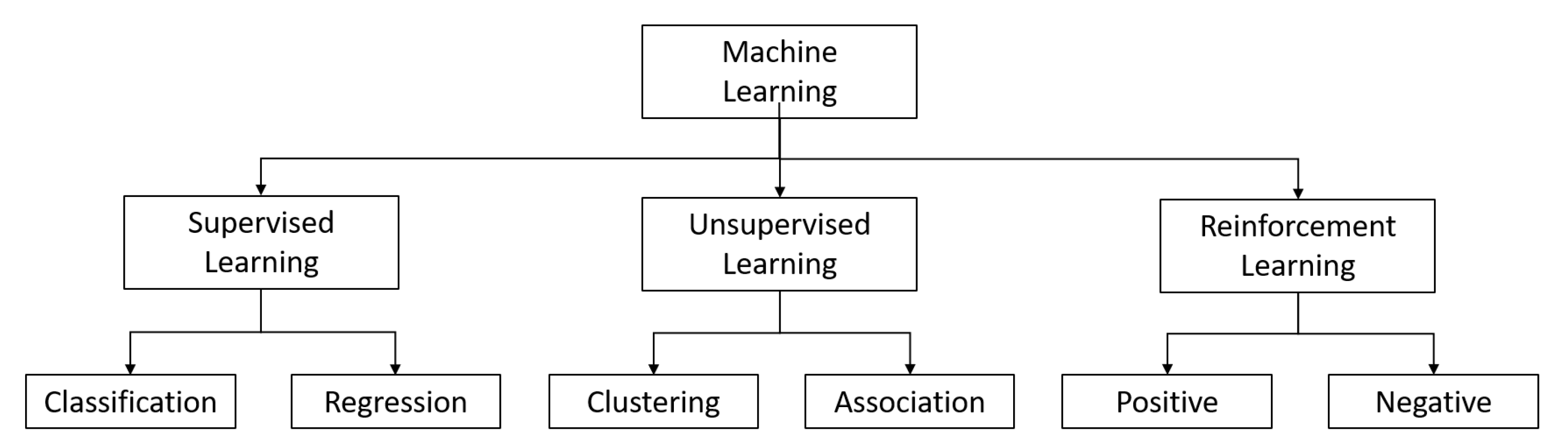
ML can broadly be defined as the capability of a computer program to improve automatically with experience via the performance of certain tasks. A performance measure quantifies this experience, and if it improves, we say that the machine is learning [33]. As shown in Figure 2, ML can be classified into three types: unsupervised, supervised, and reinforcement learning.
In learning tasks, we usually aim to estimate one or more output variables for a given set of input variables . When the desired output variables Y are in hand, the learning task is dubbed as supervised learning or metaphorically learning from a teacher [34]. In other words, we know the correct answer, and we try to learn the dependency between input variables X and Y. At the same time, one can take as random variables since many factors may influence data and measurements, making the whole setting stochastic [25]. Then, we can represent these random variables by a joint probability density . In this case, a supervised learning is concerned with determining the properties of the conditional density function . Output variables Y could be class labels (classification) or real numbers (regression), possibly resulting from the coding of unstructured data [35].
When the desired target variables Y are not obtained, the learning task is called unsupervised learning or learning without a teacher [34]. In this case, the training only involves the n observations of random variables X with joint density , and the goal is to directly infer the properties of this probability density function. These properties can be finding the joint values of the variables that frequently appear in the data (association rules), grouping or segmenting a collection of similar or dissimilar samples into subsets (clustering), or the projection of data into lower dimensions usually ranked by variance (dimensionality reduction). Unsupervised learning is typically concerned with finding patterns in the data and thus, is close to data mining and knowledge discovery in databases [35].
Existing somewhere between supervised and unsupervised learning, semi-supervised learning is based on extending either unsupervised or supervised learning to include additional information typical of the other paradigm. Two main settings of semi-supervised learning are semi-supervised classification and constrained clustering. The former is a classification task with partially labeled data (usually useful when the training sample size is small). The latter is unsupervised learning with some sort of supervised information about the clusters [36]. Recently popular, active learning methods are a subset of semi-supervised machine learning. The idea behind active learning is that a machine can learn with less training data if it is allowed to choose from the training data set by asking questions [37]. A comprehensive review of these methods for application in (geo) text and image classification is available in [32].
Finally, in reinforcement learning, the machine produces some actions and interacts with its environment. These actions affect the state of the environment and, in turn, it receives some scalar rewards (positive reinforcement learning) or punishments (negative reinforcement learning). The goal of the machine is to learn to act in a way that maximizes (minimizes) the future rewards (punishments) [35]. Deep reinforcement learning has been used for navigation tasks [38], autonomous driving [39], spatial dynamic and agent based systems, and some other domains [40,41].
Regardless of the type of ML and its task, when spatial data are used, we need to account for their properties. Before reviewing the best practices on ML of spatial data, we review the main properties of spatial data in the next section.
3. Spatial Data Properties
In machine learning, observations are represented by a matrix X where the rows are instances (samples) of a phenomenon under study, and columns are different attributes associated with each of these instances. The same applies to spatial data, but the samples on each row are also referenced to a specific location in the geographic space. To define the relationship between the real world and this matrix, we can choose between two well-known views of the world, namely, the field view or the object view [42]. Field entities are usually represented by regular grids and object entities by points, lines, or polygons. Being referenced to a specific location in space creates unique properties for spatial data that geographers and econometricians have studied over the years [43,44,45]. There is a broad agreement in the literature that there are three fundamental properties for spatial data: spatial dependence, spatial heterogeneity, and scale.
3.1. Spatial Dependence
Named the first law of geography by [46], “near things are more related than distant things” formulates the first property of spatial data, which is known as spatial dependence. Spatial dependence is a fundamental and useful property of spatial data that stems from the general continuity of space. A variety of ways exist to express and measure spatial dependence in data sets. For example, a spatial autocorrelation statistic can summarize the similarity of the values for a variable of interest at different locations as a function of the distance that separates them or of their adjacency to each other [47,48]. The Global Moran’s I is an indicator of spatial autocorrelation and is a similarity index, which is usually used for areal data. It is calculated based on the cross-product of variations from the mean [49]:
where and are the attribute values at sample locations and , respectively. is the sample mean and is the sample variance. Weight matrix element represents the spatial relationship between paired geographic units, which can be defined based on contiguity (topological relationship of spatial units) or distance (distance is determined on a physical or social network, 2D or 3D Cartesian space). The I index takes positive or negative values between −1 and +1. A positive value means similar values happen in close proximity, while a negative value shows that dissimilar values are spatially grouped close to each other. A value close to zero shows no spatial autocorrelation for the variable, indicative of a spatially random process; in the latter case, the assumption of independence, essential for many statistical methods, is met. More measures of spatial autocorrelation have also been suggested, such as Geary’s C [50], which considers the square of variations of the variable between two locations.
Alternatively, semi-variogram analysis (see [51]) can be conducted to estimate the spatial autocorrelation structure of a stochastic process based on the variance of the observations over a range of distances (usually for geographic phenomena represented by points). The empirical semi-variogram is defined as half of the average squared difference between values of a random field Z at pair points and for a given distance h in a region:
where is the number of pairs of points located at distance h from each other. The semi-variogram is visually analyzed in a variogram. A range parameter is defined as the distance beyond which spatial autocorrelation disappears in the data, thus expressing the spatial dependence structure. In principle, the spatial autocorrelation decreases as the distance among geographic units increases [52]. From a statistical point of view, spatial dependence violates the assumption of independence and identical distribution (i.i.d.), central to many statistical methods. While this assumption is not required for ML methods, spatial dependence properties still need to be considered for some applications and may significantly contribute to enhancing the quality of the learning process, which will be discussed later (see Section 4.1.1).
Two more complex components of spatial dependence are the neighborhood effect and spillover effect. While the spatial weight matrix is usually used to capture the spatial dependence of the dependent variable, spatial association rules, which are based on linguistic or topological (in mathematics language) rules, are used to capture these two more implicit spatial effects. Association rules such as, “if block group A is next to a high crime neighborhood, then block group A has high crime” (neighborhood effect) or “if a block group A is next-to a shopping mall, then block group A will experience high crime” (spillover effect) are examples of these implicit spatial effects [53,54]. However, most traditional machine learning algorithms do not consider the impact that the spatial dependence property may have on learning these association rules. For example, while we expect the crime rate at a block to be more similar to its neighboring blocks than the farther blocks, traditional machine learning algorithms, such as support vector machines (SVM) or neural networks have not been designed to incorporate this characteristic [25].
3.2. Spatial Heterogeneity
All patterns that we can observe result from the four main processes, namely, interaction, dispersion, diffusion, and exchange over the geographic space [42]. A specific observed pattern can be the result of one or multiple processes. These processes may happen in different spatial as well as temporal scales, over varied durations, and with differentiated intensities. A mixture of those with the place-based environmental factors and contexts (which are the existing patterns resulted from interweaving previous processes at that location) in different sub-regions creates even more complex patterns of outcomes [55,56].
Global measures of spatial autocorrelation may confirm the existence of positive or negative self-similarity with regard to distance, but this comes at the cost of a fundamental assumption. The parameters (mean and variance) of the random function representing the process are assumed to be constant, which means that the sample’s distribution is even over the extent of the territory over which data are generated. This is called the stationarity of the random function associated with that process [51], and when it is violated (called a nonstationary process), the process is heterogeneous. In other words, a spatial process is said to be stationary when the difference between values of an attribute is only explained by the distance between the points or units [57,58]. Another source of spatial heterogeneity is when the spatial dependence is different in various directions (anisotropy). For example, high precipitation patterns may be interrupted in a specific direction where the spatial topography of the terrain (mountains) blocks the clouds [30]. Spatial heterogeneity is not limited to the geo-spatial domains and has been studied in other domains, such as molecular biology of the cells [59] and neuroscience [60].
3.3. Scale
Scale is also important because it can inform about sampling for training experience. Learning is more reliable when the distribution of the samples in the training experience is similar to the distribution of the test experience [33]. In many geographic studies, training occurs on data from a specific geographic area. This makes it challenging to use the trained model for other geographic regions because the distribution of the test and train data sets is not similar, due to spatial heterogeneity [61]. This means that the sampling strategy for the training data set is essential to cover the heterogeneity of the phenomena of interest over the spatial frame of study. The scale can inform the sampling of the training data set by defining its elements, namely, resolution (measurement scale), context (scale at which the process is operating), and spatial extent (extent of observation) [62]. By increasing the extent of the study area, more processes and contextual environmental factors may alter the variable and result in non-stationarity by interweaving spatial patterns of different scales or inconsistent effect of processes in different regions [63]. This is especially important because collecting spatial samples is an expensive undertaking.
There are two distinct challenges related to scale and zoning when working with spatial data with areal units: the modifiable areal unit problem (MAUP) and the uncertain geographic context problem (UGCoP). The first notion is related to the sensitivity of the analytical results to the definition of the geographic units for which data are collected [64]. Ref. [65] demonstrated how different levels of spatial aggregation and zoning could result in different values of the correlation coefficient for areal units. They generated two variables with high positive and negative spatial autocorrelation and investigated the effect of varying levels of aggregation in the correlation coefficient. The results show that even in the absence of spatial autocorrelation, the correlation coefficient increases by grouping and aggregation. Attempts have been made to provide solutions for the MAUP problem based on the size and interconnectedness of the areas [66] and spatial entropy [67,68].
The second problem, UGCoP, refers to the sensitivity of the contextual variables and analytical results to different delineations of contextual units [69]. Kwan highlighted how varying delineations of contextual units, even if everything else is the same, can lead to uncertain and inconsistent analytical results over time. Note that this problem is different from the MAUP because it refers to the contextual influences on the individuals being studied in geographic units with unknown or uncertain spatial configuration. In this regard, it is closer to the ecological fallacy [70] problem, which relates to inferences about individuals from inferences in the aggregated level. An example is in environmental health studies, where residential neighborhoods (e.g., census, postal code, or buffer) are typically used as contextual units. However, these geographic units may not accurately represent the actual areas that apply contextual influences on the health outcome. People are exposed to health risks in different locations (home, school, etc.) during the day, and it is not easy to delineate the boundaries of such exposures. UGCoP is not due to different zoning or spatial scale, but contextual influences naturally change across granularities, making it even more complicated to delineate geographic contextual units [69].
The scale of analysis and appropriate geographic contextual units are among the first questions that one may need to answer before applying any spatial machine learning. However, the above-mentioned fundamental problems have rarely been investigated in spatial machine learning applications. For example, ref. [71] showed how MAUP can lead to perturbations in the convolution-based residual neural networks used for urban traffic prediction. Thus, the investigation of such effects on spatial machine learning is critically needed.
3.4. Other Properties
In addition to the above main properties of spatial data, some less fundamental but still essential properties may result from the specific representation of the data (polygon, line, point, regular grid, text) or the process of measurement [42]. For example, discretizing the continuous space into pixels may cause a loss of information at the sub-pixel level [72], while delineating the boundaries of geographic regions entails some generalization and may not be easy, due to the Boolean nature of typical regionalization approaches [73]. When working with text data, disambiguation in place names and addresses due to multiple instances for a single entity, a single entity with multiple names, and different addressing systems can create uncertainties [14,16,74,75]. Additionally, the geometric interpretation of vague place names, such as ‘midland’ or ‘near’, is usually not straightforward [76,77].
Moving from a 2D spatial space to a 3D space may impose some limitations and create some biases when ML applications are used. An example would be the case of 3D point clouds. The density of the point cloud usually changes by distance from the sensors: the closer the sensor, the higher the density. The implication of this effect is that identifiable spatial features in more dense areas of the cloud may not be recognizable in more sparse areas [78].
Finally, for many image-based applications (less for satellite images and more for close-range images), the orientation of the sensor at the time of capturing the image may influence the amount of energy received by the sensor. This makes orientation an important element. A case susceptible to such an effect in remote sensing would be that of night light images, where satellite viewing vertical and zenith angles can significantly impact the amount of light in urban areas [79]. Statistical models are commonly used to handle these characteristics in remote sensing. In close-range photogrammetry and computer vision applications, however, the sensor’s geometry at the time the image is captured is usually reconstructed. Interested readers are referred to the famous structure from motion [80] and visual simultaneous localization and mapping (Visual SLAM) [81]. As for applications in ML, the simplest way to make the model invariant of the orientation is to train the model with samples from different orientations and image augmentation. In the next section, we categorize the literature into two pathways through which spatial properties of data can be handled.
4. Machine Learning of Spatial Data
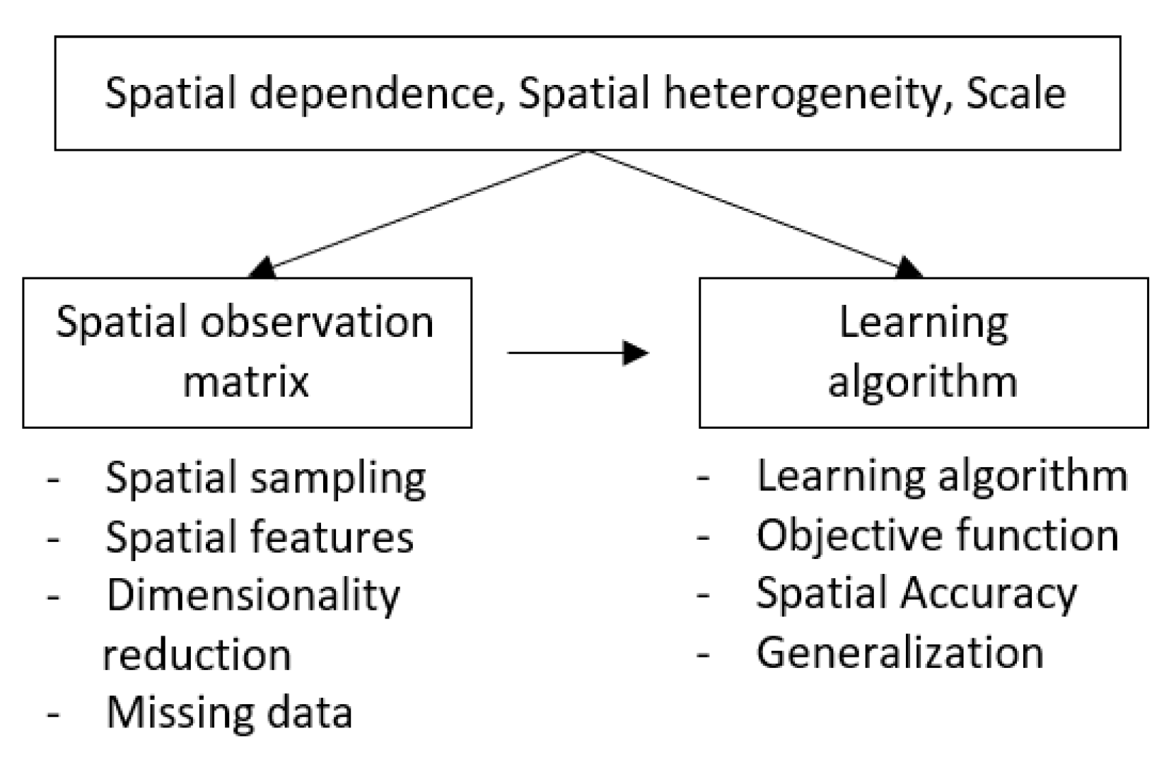
To conduct machine learning of spatial data, we need to add location, distance, or topological relations to the process of learning. Figure 3 organizes the learning process into two steps, the spatial observation matrix and the learning algorithm. We review the literature to address how spatial data properties can be involved in each of these steps.
4.1. Spatial Observation Matrix
One typical way to include spatial properties in ML is to find a representation for these properties in the observation matrix X. The principle here is that, after we design and engineer the observation matrix X to include spatial properties, we can effectively use typical ML methods (e.g., families of decision trees and random forests, support vector machines, neural networks, and ensemble models) without making any changes to the learning algorithm. Several critical aspects are involved in creating an ultimate spatial observation matrix used as an input to the learning algorithm, namely, spatial sampling, spatial features, dimensionality reduction, and handling missing data. These are discussed hereunder.
4.1.1. Spatial Sampling
While tremendous progress has been made in spatial data collection technologies, ML methods still face essential challenges in acquiring optimized samples for training. The current view in ML is to move from model-centric ML to a more data-centric ML [82]. From a statistical point of view, the size and distribution of a sample set should represent the entire population or distribution. Two important points need to be made here. First, this is distinct from the commonplace concern about the poor arrangement of samples in training and test data sets in ML, which leads to a typical generalizability issue (see Section 4.2.11 on this matter). Instead, the entire sample set (including both the training and test data sets) should represent the phenomenon being learned, which is a sampling problem [83].
Second, the representativeness of the samples is defined in the attribute, spatial, or temporal space (or multiple spaces at a time) depending on the application. The structure of the data in each space may impose some special properties. As far as the spatial data matrix is concerned, data properties in a spatial space, such as spatial dependence, can inform an optimized sampling configuration to avoid redundancy.
It is not always the scarcity of the samples that leads to challenges for learning. Oversampling will not impact the learning process because the assumption of i.i.d. is not required in ML [84]. However, it may overestimate the accuracy of learning in the assessment process. For example, let us consider a land cover classification task, using satellite imagery. Suppose that a large batch of samples are selected from close locations for a single class category (e.g., vegetation). It is most likely that these samples are similar to each other. In this case, even if samples from other sites are available in the sample data set, the classifier is somehow biased since it most probably labels the frequent familiar samples correctly. Thus, the confusion matrix class accuracy and recall, which are usually used to evaluate classification results, are not robust to assess the learning results with the varying sample sets [85,86]. This problem is known as intra-class imbalance [87]. Intraclass imbalance is not solved by cross-validation methods typically used in the generalization step (Section 4.2.11). This means that we either need an evaluation method that can account for such effects or to be careful in sampling the data that enter the learning algorithm. For a useful review of the spatial sampling methods, see [52]. It is worth noting that inter-class imbalance in which the number of samples in class categories are highly uneven can also degrade the accuracy of classification. The performance on a class with many samples will be higher, compared to the classes with fewer samples. While it overestimates the overall accuracy, inter-class accuracy is still identifiable by looking at single class accuracy and recall in the confusion matrix [88].
One application of reinforcement learning is for efficient spatial sampling. Over space, sampling can be conducted adaptively, according to local contextual characteristics using reinforcement learning. For example, Ref. [89] trained an agent to select appropriate spatial resolutions for satellite images that run through detectors. When a low spatial resolution image is dominated by large objects, the agent passes this image to a coarse level detector. Alternatively, when a high spatial resolution image is dominated by small objects, the agent passes that image to a fine level detector. Such an approach reduces dependency on high spatial resolution images that are more expensive and need more time to process. One of the problems in object detection algorithms is that the algorithm must use a sliding window that passes exhaustively through the entire image to detect an object. Ref. [90] presents a reinforcement learning method to select a small set of sequential samples from the image before deciding whether a target is present in an image.
4.1.2. Spatial Features
Several methods exist to include the spatial components of data in the observation matrix. One way is to directly add the spatial reference to the data matrix as attributes. This entails embedding the spatial references of data directly into the attribute space. Practically, this can be implemented in either one of two ways. One consists in adding coordinates (e.g., latitude and longitude) alongside semantic attributes for each observation to the observation matrix [91,92]. For example, in [93], the authors demonstrated that in many propagation environments (e.g., in sensor networks deployed in outdoors for environmental monitoring), where the wireless channel strength is a function of the distance dependent path-loss, adding the geographic location of transmitters and the receivers as input to a neural network model can efficiently schedule links between transmitters and receivers. Such a capability is important in dense sensor networks in which simultaneously activated nearby links (connections between transmitters and sensors) produce significant interference for each other. However, using the coordinates as spatial variables may generate considerable overfitting because they are highly correlated [94]. The other typical way is to add observations tied to a region as fixed effects of that region to the observation matrix [95,96]. This approach is effective to handle inclusion relationships; however, it cannot capture complex structures.
In addition to spatial reference information, spatial entities and phenomena have within-object information (geometric, spectral, textural, and statistical) and between-object information (contextual and relational), which can be created as new features and added to the observation matrix directly [1]. The geometric information of single spatial entities can be used in different forms such as the length, area, and ratio thereof. Spectral and textural information have extensively been used in the remote sensing community for land-cover and land-use classification. However, spectral features are insufficient for this purpose due to heterogeneity, especially in urban environments [2].
Other features, such as texture, which indicates the coarseness or smoothness of a pattern in an image, have been suggested as complementary information. From a mathematical point of view, numerous functions exist that can represent the local variability of pixel values as texture features, including first-order statistics (e.g., means, variance, and standard deviation) and second-order statistics (gray-level co-occurrence matrix, spatial autocorrelation) [97]. These methods, however, focus on a single scale. Multi-resolution spatial and frequency analysis tools, such as Gabor transform, Wigner distribution, and wavelet transforms, have effectively been used to overcome this problem [98,99,100,101].
Texture analysis is usually conducted using moving windows (regularly shaped grid) or fields (irregular shape). Compared to moving windows, fields partition the area into homogeneous regions and provide a more realistic representation of the spatial entities [97]. The boundaries of these fields are determined using existing polygon features or digital image segmentation methods (e.g., edge detection, region growing) [102]. In addition to textural and spectral information, geometric and contextual attributes of the fields can also be used. In this respect, [103] used the proportion of build-up area, vegetation, and water surfaces, and [104] calculated the spatial metrics for land covers and semi-variogram for the Normalized Difference Vegetation Index (NDVI).
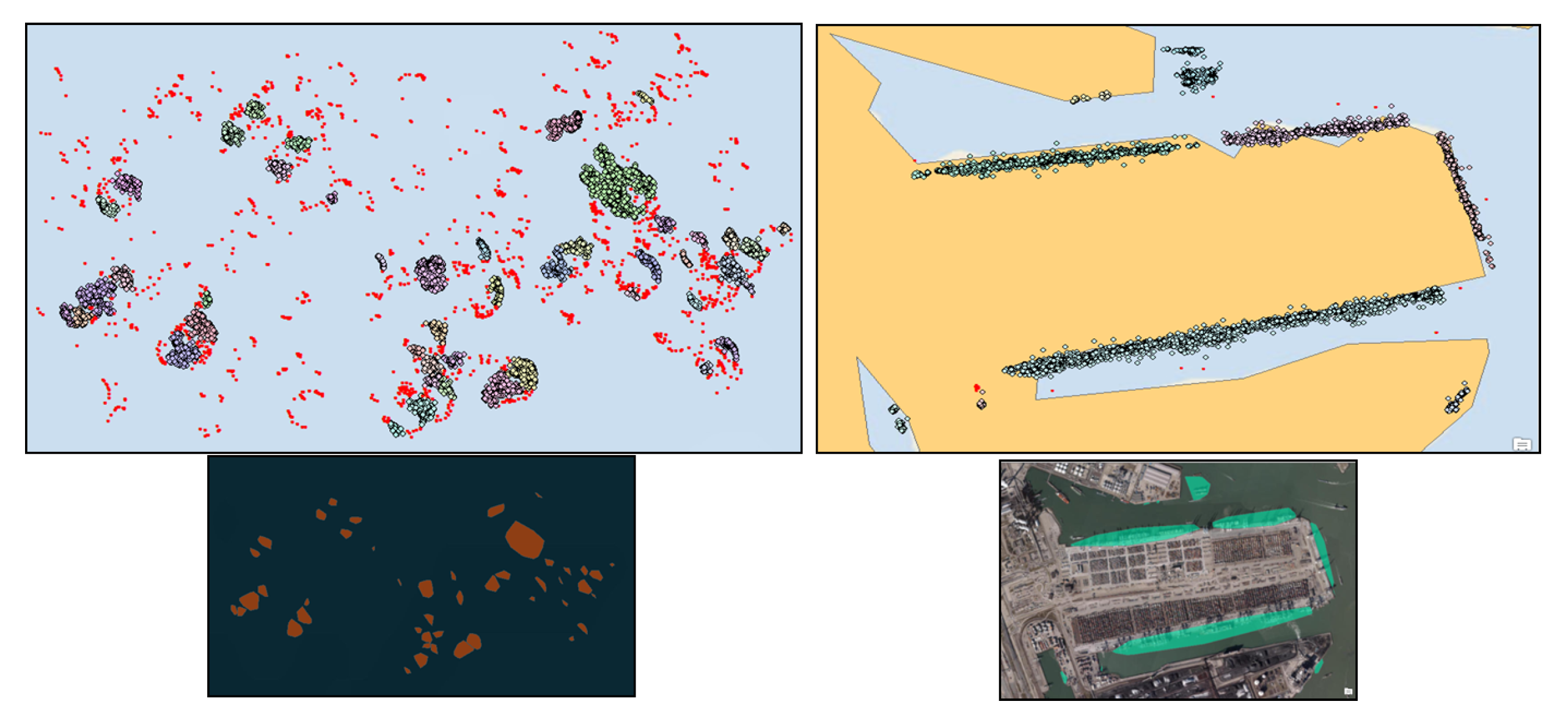
We provide here another example of how to identify and delineate the boundaries of functional zones based on moving object patterns. Figure 4 shows two zones inside and outside the port of Rotterdam, the Netherlands. The points represent the recorded location of vessels that visited an unlabeled zone, extracted from the vessel trajectories’ stop and move segments. On the one hand, the point clusters may inform about the boundaries of each zone. On the other hand, shape and simple statistics within each zone, such as the duration of visits, the number of unique vessels, distribution of vessel course (direction), and vessel type, may provide some information about the functionality of space (e.g., anchorage, containerized ship berth, bulk ship berth). This within entity information can be added as new features to the observation matrix to recognize the functionality of the zones.
Further, between-objects information, such as connectivity, contiguity, distance, association, and direction, can be used to create new features [1]. In the vessel movement example, the association of zones, where different types of ships dock to load and unload cargoes in close distance, may become a discriminating feature to distinguish the port area from anchorage zones outside of the port (in Figure 4, compare bottom-left and bottom-right quadrants).
Point cloud classification is another area where machine learning methods have been used extensively. The simplest way to classify point clouds is to add the third coordinate as an attribute of each point and use standard 2D ML methods to classify the point cloud. However, there are two critical shortcomings for such approaches [78]. First, point clouds may have multiple z values for a point with (x,y) coordinates, and compression of the 3D point cloud to 2D image causes a loss of information. Second, points in point clouds are usually irregularly spaced, making the selection of a fixed window size difficult. In other words, the point densities may vary in relation to the distance to the sensor. As a result, features learned in a dense area are not generalizable to sparse areas.
Ref. [105] used regularly spaced voxels and voxel feature encoding (VFE) to address the first problem. This method is subject to loss of information, due to decreased spatial resolution and increased memory usage in the voxelization process. Alternatively, Ref. [106] projected point clouds on multiple synthetic 2D images and labeled pixels based on the prediction scores from these synthetic images to handle the first issue (Figure 5a). Ref. [78] suggested creating a point cloud pyramid with l scale levels by subsampling the original point cloud. The deep hierarchical features (see Section 4.2.6) for each point are extracted using a deep neural network within each scale. Such an approach forms a feature pyramid (Figure 5b). The feature vectors of a point along this pyramid are concatenated to create a final feature vector that is fed into a classifier. This final feature vector contains both hierarchical and multi-scale features of the original point cloud, which can address both issues discussed earlier.
4.1.3. Dimensionality Reduction
ML tasks may end up with a large number of input variables in the observation data matrix. A disproportionately large number of interrelated variables may negatively impact learning in a variety of ways. Apart from the need for more training data and an increase in processing time, an unnecessarily large number of variables may impose new uncertainties into the learning process because of the correlation between variables [107]. One way to handle such a problem is to select a subset of features that provide the best results. A variety of methods exist for feature selection, such as a genetic algorithm [108]. Dimensionality reduction methods are another way to handle many useful variables, especially when the influence of each variable is not of interest.
To reduce unnecessary variables, we need to understand the structure of the variance–covariance matrix. The problem is that calculating the variance–covariance matrix for a given observation matrix is computationally expensive for a large number of variables. Several dimensionality reduction methods exist, including but not limited to principal components analysis (PCA), factor analysis, independent components analysis, and self-organizing maps (SOM) [109,110,111]. PCA is a statistical method well known for its application in dimensionality reduction. PCA transforms the observation matrix with many interrelated variables to a smaller set of new uncorrelated variables (components). These new variables are ordered so that the first few retain most of the variation present in the original variables [110].
It is proved that by applying useful linear algebra operations, C can be decomposed into , where L is a matrix of eigenvectors (representing the weight of each variable on corresponding principal components), and V is an orthogonal matrix of eigenvalues (representing the variances of the corresponding principal components). The observations are then transferred to a space where the column vectors in L represent the axes. In practice, a few principal components that represent most of the variation in the data set are selected (Figure 6). These transformed observations are then entered into the learning algorithm.
For an observation matrix with spatial references, a simple PCA assumes the structure of the variance-covariance matrix remains stationary across the study area. Ref. [112] showed that PCA could be weighted locally either in attribute space (LWPCA) or in geographic space (GWPCA) to account for certain heterogeneities. For the former, we assume the covariance structure is homogeneous for observations that are close to one another in attribute space, which leads to with respect to the sub-region i. The GWPCA for location , however, is written as , with as the variance–covariance matrix of location .
While PCA is a common approach in summarizing (sub)sets of variables in ML, LWPCA and GWPCA have not been investigated. Such methods can additionally provide insights into the spatial distribution of each composite variable by mapping components scores. This may lead to a complete understanding of the process [113]. Moreover, eigenvalues and eigenvectors can be obtained for locations with no observations. Challenges include bandwidth selection and more computational cost. A locally weighted PCA can also optimize sampling re-design by identifying local and spatial outliers rather than global and aspatial outliers [112].
4.1.4. Missing Data
Nowadays, data are more available, both spatially and temporally. However, given that they are more often organic, being a byproduct of the processes that created them in the first place, there are always gaps in temporal and spatial dimensions because of effects and circumstances that are out of our control. Therefore, missing data is an important challenge, and many analyses are simply not implementable without having a way to deal with this problem. Missing observations can be independent of each other, dependent on their neighboring points, or with specific patterns [114]. There are different ways to address missing values, such as aggregating data into coarser granularity, removing the observations with missing values from the data set, and imputing values. Although imputing data adds preprocessing step to analysis, it leverages the existing data and avoids losing information due to aggregation and discarding some observations.
Spatial prediction methods can always be used to impute values for data sets with missing values. The most famous approaches for spatial prediction are spatial statistical models (e.g., geographically weighted regression) and geostatistical models, such as kriging [115]. Several studies have demonstrated that kriging in the universal form is preferred to geographically weighted regression for prediction, due to its optimal statistical properties [116].
Apart from the statistical and geostatistical models, other approaches in machine learning and other paradigms have also been adapted to spatial properties for missing data imputation. Probabilistic principal component analysis (PPCA), for example, is a probabilistic extension of PCA and has been used to impute missing values for different applications [114,117]. This method has proven useful when a significant portion of the observation matrix is unknown [118]. A comparison of different types of PPCA can be found in [119], and an extension of PPCA to consider temporal and spatial dependence can be found in [120]. All systematic errors must be removed before using PPCA for imputation [114].
4.2. Learning Algorithm
Instead of generating new spatial features and processing them with traditional non-spatial machine learning methods, we can directly incorporate spatial properties in the learning algorithm. Among all ML methods, decision trees and random forests, support vector machines (SVM), neural networks, and deep neural networks (DNN) have found considerable attention in spatial science.
4.2.1. Decision Trees
Decision trees (DT) are popular ML methods adapted for spatial problems to overcome violation of the i.i.d assumption. As a class, spatial entropy–based decision tree classifiers use information gain coupled with spatial autocorrelation to select candidate tree node tests in a raster spatial framework. For example, Ref. [121] added a spatial autocorrelation measure to the target function evaluated at each node of the tree. PCT is a multi-task approach where hierarchies of clusters of similar data are identified, and a predictive model is associated with each group. When splitting a group is considered at a node, a test is run that maximizes within-cluster variance reduction. To account for spatial non-stationarity in the target variable, a term based on global measures of spatial autocorrelation was added to this test.
A common trait of such approaches is to add a constraint to account for spatial properties, while still relying on local entropy testing at tree nodes. One of the frequently occurring issues in image classification using decision trees is salt and pepper noise. Salt and pepper noise happens when the predicted label of a specific pixel differs from its neighborhood pixels and can result from high spatial autocorrelation in class labels of the sample data used for training. Ref. [122] proposed a focal-test-based spatial decision tree (FTSDT), in which the tree traversal direction of a learning sample is based on local and focal (neighborhood) properties of features. They use local indicators of spatial association-Lisa [123] as spatial autocorrelation statistics to measure the spatial dependence between neighborhood pixels.
Geographically weighted versions of decision trees have also been developed to account for spatial heterogeneity. Ref. [26] presented a geographically weighted random forest (GW-RF) to visualize the relationships between type 2 diabetes mellitus and risk factors in U.S. counties. Similar to geographically weighted regression (GWR), the spatial weight matrix and RF are integrated into a local regression analysis framework. Compared to global RF, GW-RF showed higher variability of the type 2 diabetes prevalence. One downside of GWR when interpreting the importance of the variables is that it overlooks collinearity among the predictors, which leads to parameter redundancies. Thus, any attempt to interpret a local coefficient independent of the other local coefficients at the same location is not valid. RF-GWR, however, is not impacted by collinearity [124].
4.2.2. Support Vector Machines
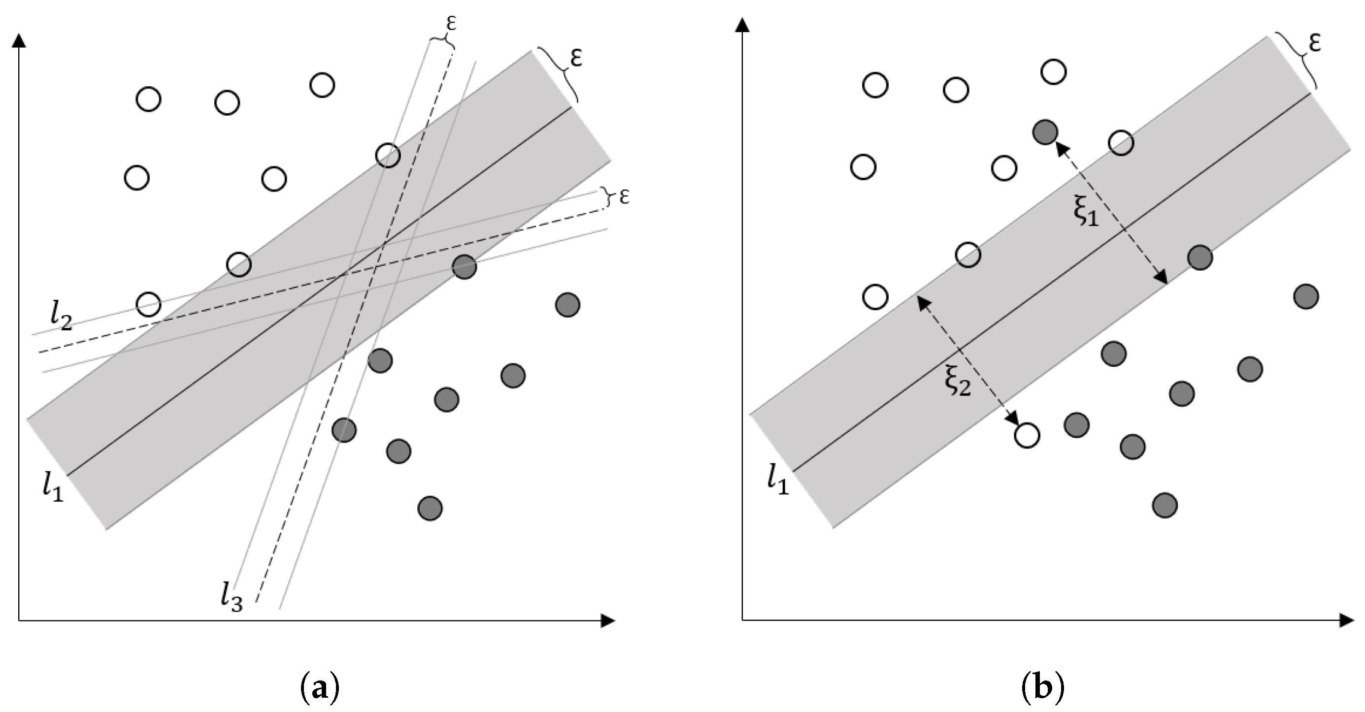
Support vector machines (SVMs) have been used for classification and regression problems [125]. The idea of SVM is to map the original input space to a higher-dimensionality feature space where the observations are separable by hyperplanes (Figure 7a). Among all possible hyperplanes, the one that maximizes the margin width () is optimized (). In reality, observations may not be separable easily, due to the presence of outliers (Figure 7b). Instead of increasing the complexity of the model structure (in this example, a nonlinear curve), we allow misclassification of some observations and penalize them based on their distance from the margins (). In essence, the objective function has two terms: a term containing and another term containing , and the goal is to maximize the former and minimize the latter. is called a regularization term. Regularization terms are usually added to objective functions to control the complexity of the model and avoid overfitting (see Section 4.2.11). SVM performs well in high dimensional spaces. It is less sensitive to class imbalance and powerful in generalization [11].
Ref. [126] suggested an extension of SVM called support vector random field that explicitly models spatial dependencies in the classification using conditional random fields (CRF). The model contains two components: the observation-matching potential function and the local-consistency potential function. The former models the relationship between the observations and the class labels using an SVM classifier, and the latter models the relationship to neighborhood labels. The local-consistency potential function penalizes discontinuity in between the pairwise sites.
4.2.3. Self-Organizing Maps
Self-organizing maps (SOM) are among nonlinear clustering methods that have been used with spatial and non-spatial data [111]. SOM is a simple neural network with no hidden layers. It maps an n dimensional feature vector to a regular grid of square (four neighbors) or hexagons (six neighbors) neurons in the output layer, initialized with n weights. First, a similarity measure is used to find more similar neurons to the input feature vector. Then, the weights of the activated neurons and their neighboring neurons are adjusted to make them even more similar to the input vector. This process is repeated for a set of input feature vectors. Finally, it creates a spatial organization of the neurons in a one-, two-, or three-dimensional space in which dissimilar units stay farther away. SOM is similar to K-means clustering but different in two ways. First, K-means is based on the nearest distance, while SOM utilizes distances between all paired neurons (weighted by a neighborhood kernel) [20]. Second, SOM also visualizes the relation between clusters by representing how far they are from each other in a topological space [111]. Such a property makes SOM attractive for visual data mining. For example, it is possible to compare the SOM visualizations with other forms of visualization (e.g., geographic visualization), especially in an interactive platform [127]. Ref. [12] used SOM to visualize demographic trajectories, and [20] demonstrated how SOM could be employed to visually mine spatial interaction systems using a large domestic air travel data set. This property can even be used to map data without spatial properties in a 2D or 3D space. For example, Ref. [128] mapped massive textual databases with several hundred dimensions in feature space into a 2D space using SOM (Figure 8).
Apart from visualization, one concern about using SOM for geo-referenced data is that the geographic reference of the data is ignored in mapping. Ref. [129] suggested a variation of SOM called Geo-SOM to address this issue by considering spatial dependency. Geo-SOM forces the algorithm to search among the neurons geographically close to the data pattern when seeking the winning unit for a specific data pattern. Ref. [130] suggests using a one-dimensional SOM to create a sequence of numbers (cluster indices) that are ordered according to the similarity of attributes within the high-dimensional space. Each spatial point can then be labeled with its associated index number and represented in a choropleth map. The spatial pattern of these number sequences, called contextual numbers, summarizes the variations of geographic locations in high-dimensional space in a single contextual map (Figure 8b). Like other dimensionality reduction methods in Section 4.1.3, such a feature (with the advantage of being a nonlinear dimensionality reduction method) can be used as input to machine learning. For a complete review of SOM applications in GIS, see [127].
4.2.4. Radial Basis Function Networks
Radial basis function (RBF) networks have an input layer, a hidden layer, and an output layer. Instead of a linear relationship between the input vector and the neurons in the hidden layer followed by a nonlinear activation function, the weighted norm (distance) of the input vector and the neurons are calculated in RBF networks with a radially symmetric activation function, which is usually Gaussian. Ref. [131] compared the RBF network with MLP networks for modeling urban change, and showed that RBF demonstrates higher prediction accuracy. Ref. [132] used the RBF networks for spatial interpolation by incorporating a semivariogram model where the neurons in the hidden layer are the center of the observation points. Ref. [133] demonstrated how a hybrid MLP-RBFN network can improve the spatial interpolation results, where MLP and RBF collaborate to fit surfaces of different types.
4.2.5. Adaptive Resonance Theory Networks
Adaptive resonance theory (ART)–based networks are a family of neural networks that have been used in spatial interaction flows, crop classification, and land-use change applications [134,135,136]. ART-based networks are supervised, self-organizing, and self-stabilizing neural networks that can learn fast in nonstationary environments [137]. Fuzzy ARTMAP, which couples ART-based networks with fuzzy logic, is the most famous ART-based network [138]. It includes two input modules: and , each with two layers connected by a map field module. matches the input vector to the most similar neurons in its second layer. If the vector is not similar to the current neurons in memory, a new neuron is created. This property enables the neural network to adaptively change the topology of the network and adds new experiences to the memory. , which maintains the class labels, is connected to through a map module. However, the Fuzzy ARTMAP depends on the quality of training data and sensitivity to noise and outliers that may be treated as novel patterns. Ref. [134] used the adaptive nature of the Fuzzy ARTMAP in forming its topology to account for spatial heterogeneity in land-use change. Their proposed ART-P-MAP considers the land-use change as a regression problem instead of a classification problem and uses the density of training observations as a confidence measure for prediction through a Bayesian decision approach. This approach increases the generalizability of the model and avoids the problem of adding new neurons due to noise and outliers.
4.2.6. Deep Convolutional Neural Networks
In the past few years, deep neural networks (DNNs) have been proven as more promising to process data in their raw form than conventional ML methods. DNNs are usually composed of several nonlinear but simple modules that represent data at different levels. Starting with raw data, each module transforms the representation at one level into a representation at a higher (more abstract) level. In the process and using the backpropagation algorithm, the machine can learn very complex functions [139].
Popular DNNs for spatial data can roughly be classified into four categories, namely, convolutional neural networks (CNNs), deep graph neural networks (GNNs), generative neural networks, and recurrent neural networks (RNNs) when combined with CNNs. Here, we discuss several main DNNs that can consider spatial properties of data in their architecture or have been used to solve problems in spatial domains starting with CNNs. RNNs are used primarily to learn from sequence data and will be discussed in Section 5.
CNNs are the most popular and well-established form of DNNs to process and analyze images. They include convolutional layers and pooling layers as the two main types (Figure 9a). Convolutional layers work based on convolution of a sliding window (filter) with pixel values across the image Figure 9b. The filter weights are determined automatically through the learning process by the network. This is the main advantage of deep CNNs in comparison to conventional ML methods where user defined filter weights are needed. This feature of CNNs has been used on a limited basis to automatically define W matrix weights in other spatial applications [24]. Pooling layers aggregate neighboring pixels into a single pixel, reducing the image’s overall dimensions [140]. As the number of convolutional and pooling layers increases, the network becomes deeper and can extract more abstract features. A classification network finally follows the processing of these layers. In the past few years, several prominent CNN-based DNNs have also been introduced for semantic segmentation (labeling pixels as opposed to image patches) using deep residual networks with less complexity and depthwise separable convolutions, which reduces the computation time and the number of network parameters significantly [141,142,143,144,145].
Two main differences exist between deep convolutional networks and conventional ML methods [140]. First, CNN makes the manual spatial feature extraction described in Section 4.1.2 an automatic part of the learning algorithm, that is, weights of the convolution filters are not known a priori but are instead determined through the training process, which in some ways resembles the connection weights in ordinary neural networks. These convolution filters partially account for spatial dependence properties by considering the neighborhood pixels, but their size and number within each layer must still be determined in a hyperparameter optimization process. These regularly shaped filters cannot account for variation of spatial dependence in different directions. Second, pooling operations in CNNs allow them to consider hierarchical features in training. The number and architecture of convolutional and pooling layers is arbitrary to some degree and can cause unnecessary complexity of model. Thus, one should always optimize these hyperparameters.
The input images have a regular shape in CNNs, while actual objects and regions might be irregularly shaped in the real world. An example of this is in urban land use classification. A regular shape input image may ignore the real boundaries of objects [1]. Attempts to address this problem include proposing an object-based convolutional neural network (OCNN). This approach involves a two-step process, where image segmentation is initially applied to partition the image into two object categories of linear shaped (e.g., roads) and general shaped (e.g., buildings) objects with homogeneous spectral and spatial properties, using the mean-shift method [146]. Two separate CNNs are trained on these categories of objects with different input image sizes. For linear objects, a small input image size and for general objects, a large input image size performs better. While this approach outperforms regular deep image segmentation networks, it has some limitations. First, it depends to the accuracy and robustness of the segmentation process. The extracted partitions do not necessarily represent the actual boundaries of objects. Second, the segmentation itself is a time-consuming operation, and parameters of segmentation are still needed to be defined manually by the user.
4.2.7. Deep Graph Neural Networks
Graphs have been used as a data model to represent many spatial entities (e.g., street networks) and relations (e.g., socioeconomic relations). Compared to regular grids and Euclidean spaces, graphs are irregularly structured (i.e., irregular neighborhood relationships). Thus, many of the machine learning methods cannot directly be used on graphs to perform tasks such as classification (e.g., role of a node in a social network), prediction (e.g., whether or not a social relation exists between two nodes), and community detection (e.g., discovery of criminal groups) [147]. For example, CNNs have been applied quite extensively for image classification and segmentation. However, many problems (e.g., social and biological networks) usually cannot be represented in grid format, making it challenging to apply convolutions. Additionally, feature engineering is needed every single time when conventional ML methods are used for graphs [148]. In recent years, a lot of interest has been directed toward developing ML and, especially, deep learning methods that are directly applicable to graphs. These methods are called graph neural networks.
Graph neural networks were first introduced by [149]. The main idea behind graph neural networks is to aggregate features from neighborhood nodes to represent the feature value of a node [150]. This process is similar to applying convolutions on regular grids. Thus, attempts have recently been made to generalize convolution to graphs. In general, graph neural networks can be categorized into spectral and non-spectral approaches [151]. Spectral methods create a spectral representation for the graph and apply convolution through the graph Fourier transform (using the eigenvalues and eigenvectors of the Laplacian matrix of the graph) [152,153,154]. The challenge with these types of methods is that, if the structure of the graph changes, the trained model of the previous structure cannot directly be applied to a graph with a new structure. Spectral methods are also computationally expensive and have practical issues with scalability [153]. Spatial (non-spectral) methods directly use convolutions on close neighbors in the graph [155]. These approaches are relatively new and have shown impressive performance in many applications, such as disease spread forecasting [156], traffic analysis [157], medical diagnosis and analysis [158], fraud detection [148], and natural language processing [159]. Spatial methods process the entire graph simultaneously and are computationally less expensive [150]. Graph attention neural networks are similar to the spatial graph neural networks but they assign larger weights (more attention) to the important nodes in the neighborhood [150]. Ref. [160] adopted the attention mechanism to extract the spatial dependencies among road segments for traffic forecasting, and showed attention networks perform outstanding robustness against noise. Graph neural networks can extract effective features from similar to classical CNNs on regular grids. More importantly, they can effectively reflect the true geometric structure of the original data [161].
In addition to the method that is used for learning, the chosen graph representation is important for successful learning. Ref. [162] showed how a heterogeneous representation of spatial elements in a network from OpenStreetMap (i.e., a graph with more than one node/edge type) improves the performance of a graph neural network for the semantic inference of the spatial network. As another example, Ref. [163] showed how the conventional primal (intersections represent nodes) and dual (road segments represent as nodes) representations of street networks are limited for assessing Open Street Map data quality with ML methods, and provided a hybrid representation for street networks by graph. Other novel approaches to represent spatial phenomena by networks can be found in [164,165].
A survey of deep learning methods for graphs can be found in [166]. The application of graph neural networks has yet to be explored in spatial domains, especially for non-grid-based spatial data, such as social networks.
4.2.8. Deep Generative Neural Networks
Models in ML can also be categorized as discriminative or generative [167]. On the one hand, we have discriminative models that are usually used for classification and are called classifiers. They return , the probability of a sample to belong to class Y, given the feature attributes X. Generative models, on the other hand, attempt to generate realistic features of a class of objects, given the distribution of the class . Thus, a new set of features is generated, using the distribution of a specific class. In the past few years, generative neural network models have attracted considerable attention. Among several types of generative models, variational autoencoders (VAE) (Figure 10a) and generative adversarial neural networks (GAN) (Figure 10b) have found applications for spatial prediction [168,169].
GANs were first suggested by [168]. They form a type of generative neural networks composed of two sub-networks: a discriminator and a generator. These two networks compete with one another to learn through the training. On the one hand, the generator attempts to create realistic sets of features X from data class distribution Y by adding random noise Z (Figure 10a). Random noise Z is added to make sure each time a new instance of class Y is generated. The generator attempts to confuse the discriminator by introducing this new feature set as a new instance of the class. The discriminator, on the other hand, is a binary classifier that compares with actual instances of the class and recognizes whether it is real or fake. As training continues, both networks compete until the discriminator fails to recognize the unreal instance from the actual sample. VAE works based on an encoder-decoder architecture, which has the same number of units in the input and output layers [169]. For image classification, for example, VAE creates a new representation of a labeled input image into a space of lower dimensionality; it creates a distribution of the object class in the latent space, and reconstructs a sample image from the distribution. By comparing the actual and reconstructed images, the network can learn through the training.
Many spatial phenomena are heterogeneous and nonlinear, rendering conventional data analytics methods less effective. Generative networks have been applied successfully for DEM spatial interpolation [170], spatiotemporal imputation of aerosol when a substantial amount of data is missing [171], and predicting regional desirability with VGI data [17]. However, CNN-based methods are not appropriate when a large amount of data is missing since they require complete images or images with limited random missing values for training [171]. The other application of generative models is for data augmentation, especially when the size of the training data set is small or the class balance is uneven. Data augmentation works by slightly manipulating the training data to generate new training samples [172].
4.2.9. Learning with DNNs
Apart from discussing the specific capability of the various types of networks, it is also necessary to look at the ways existing DNNs can be used. One can use pre-trained networks, adapt a pre-trained network, or train a network on new data from scratch [173]. In the first method, pre-trained models are used as feature extractors for classification problems on a new data set. This is similar to the methods in Section 4.1.2, where new features are created and added to the observation matrix. These methods have been shown to be effective at classifying remote sensing and photogrammetric imagery [174,175].
Alternatively, one can fine-tune a pre-trained network on a small set of new observations. This approach is useful when the size of the available training data set is small. One may even be able to use a network pre-trained for a problem in a very different domain or topic. For example, authors of [176] successfully fine-tuned a pre-trained network on an ImageNet data set (close range images) [177] to classify land use with a very small new training data set from UC Merced Land Use satellite images [178].
The success of fine-tuning pre-trained networks comes from the capability of models to generalize and specifically from the fact that, even though data sets may be from different settings or domains, they still exhibit fundamental standard features that machines can learn from one setting and apply to another. For example, the geometric boundary of objects in both sets of images mentioned above is composed of corners and horizontal, vertical, and diagonal lines. The way this is usually conducted is that coefficients for several layers in the trained network (usually the layers with low-level features) are frozen, and only the coefficients of the rest of the network are fine-tuned with the new observations. Compared to the first approach, fine-tuning must provide better results since features are oriented to the new data set [179]. Finally, the last method is to train the network on the new data set from scratch. However, this method is subject to overfitting if the training dataset is small [173].
4.2.10. Spatial Accuracy
Measures of the accuracy of spatial data are essential to be considered in the objective function in machine learning for a number of geospatial applications. For example, [180] showed how the lack of a spatial accuracy measure could influence the evaluation of location prediction performance for birds nests based on several habitat and environmental factors. When the variables are rasterized, one typical way to evaluate the prediction accuracy is to measure the similarity between the predicted and actual maps. In the example being discussed, a cell is labeled as either a nest or no-nest (a binary classification task). Then, the following objective function of learning performance can be used for this purpose, where a measure is devised to calculate the classification accuracy from the confusion matrix:
Figure 11a,b shows the location of sample nests and their rasterized format. Figure 11c,d represents the predicted locations in two different iterations during learning. Objective function (3) returns the same similarity value for c and d, while d is more accurate spatially. Thus, the authors suggest adding a term to the objective function to measure spatial accuracy, which could be the average distance to the nearest prediction. Therefore, we can rewrite the objective function as follows:
where is a regularizer parameter that is fine-tuned during the training.
4.2.11. Generalization
Generalization is the capability to generalize a trained model based on a set of data to future data sets. A data set is usually divided into three mutually exclusive sets, namely, a training set, a validation set, and a test set. We fit a model to our training data set at each iteration and compute an objective function to measure learning performance. Then, we use the validation data set to evaluate the model’s capability to fit another data set for generalization. This process is repeated until we have a model that fits best on both data sets. The critical point is that the validation data set is still being used in learning, and we need to ensure that our model is being tested on a completely different data set. The test data set is used for the latter purpose, after we select the best model from the previous step. More complex validation methods, such as k-fold cross-validation, can be used to guarantee the best setting of the train, test, and validation data sets [181].
If we fail to reduce the validation loss while the training loss decreases, we will have the so-called overfitting problem (Figure 12a). On the other hand, if the model is very simple, both training and validation loss are close but decrease significantly (Figure 12c). This means tha we need to control the complexity of the model to reach the trade-off between the loss value in training and the validation data set. Regularization is the method that is usually used for this purpose, which works by penalizing the weights in the loss function. We can add a regularization term to the objective function as follows:
Two famous regularization terms are (sum of the absolute value of the weights) and (some of the square values of the weights) norms. The former tosses out some of the parameters by imposing zero value to their weights, while the latter assures the weights stay close to zero. Lambda is the parameter that we need to tune to determine the best complexity level for our model and is usually domain-dependent. A small lambda value means more weight to our training data set (Figure 12a), and a large value means we are selecting a very simple model (Figure 12c). We always need to fine-tune the value for the data set to have a suitable generalization model (Figure 12b). Regularization is essential when working with small data sets that are more prone to overfitting and when we have many features that impose computational complexity and noise, which are very common when working with spatial data.
As mentioned above and in Section 4.2.8, the and values are domain-specific, which means that they need to be optimized at training time. These parameters are called hyperparameters, which are different from standard parameters, so the latter is determined based on the data set. At the same time, the former is dependent on the properties of the model [182]. Therefore, failure to choose the optimized values for these hyperparameters can cause overfitting. However, hyperparameters are not limited to regularization parameters, and their number is different depending on the machine learning method and problem formulation. For example, random forests have three primary hyperparameters: ensemble size, the maximum size of the individual trees, and the number of randomly selected variables at each node. However, in neural networks, the architecture, learning algorithm, number of training iterations, learning rate, and momentum must be set [183]. In addition, new hyperparameters may be added for spatial applications, such as the spatial accuracy, the initial size and scale of input images, size of the filters, and appropriate sample size. A detailed discussion of hyperparameter optimization in spatial science is discussed in [182].
5. Spatiotemporal Learning
A significant amount of attention has been devoted to spatiotemporal learning in the past few years with the availability of technology to collect data at a much higher frequency frequently, if not continuously. Among machine learning methods, neural networks and SVMs are used often for space-time learning. Similar to the spatial properties discussed in this paper, spatiotemporal dependence and non-stationarity may also exist in data with spatiotemporal dimensions [184]. The number of parameters in spatiotemporal ML may become very large, which can make learning impossible if the model cannot capture the underlying spatiotemporal structure well [185].
Geographically and temporally weighted regression models have already been developed for geospatial applications. Still, the challenges related to expressing complex and nonlinear space-time proximity and optimal weights for kernels remain unanswered in these methods. Ref. [24] proposed a spatiotemporal proximity neural network (STPNN) that constructs the nonstationary weight matrix instead of using fixed and conventional methods to address the complex nonlinear interactions between time and space. Ref. [22] used a multi-stage approach to address spatial heterogeneity and dependence for space-time prediction. Authors used GeoSoM to divide space and time into homogeneous regions. In the second step of the latter model, a space-time lag within each cluster was estimated to capture the space-time dependence structure among the space-time series. Finally, a feedback recurrent neural network predicts values on each cluster locally. Although such techniques have high performance, they are usually multistep, and the computational cost is high. Furthermore, complexities related to anisotropy are not modeled.
Convolutional recurrent neural networks and especially convolutional long short-term memory (LSTM) networks can be applied extensively in spatiotemporal learning of grid data [186]. LSTM is a type of recurrent neural network with the capability of memorizing temporal dependencies in data. A combination of this feature with the power of CNNs to learn the hierarchical spatial features can provide an automatic single-step ML model to account for space-time dependence (see ConvLSTM [187] and PredRNN [188]).
Recurrent neural networks have also been used in combination with graph neural networks [189]. Ref. [190] modified graph neural networks to include gated recurrent units, and demonstrated its capability on simple non-spatial graphs. Ref. [160] proposed a spatio-temporal graph neural network with attention mechanism and LSTM units to jointly learn spatial-temporal dependencies on traffic networks. Spatial dependencies are assumed fixed with connectivity and distance in all time-steps for most of the current spatio-temporal graph neural networks. However, this assumption does not hold for many real-world applications, such as traffic prediction in a road network, where spatial dependencies change dynamically based on factors, such as accidents or weather conditions [150]. A recent survey of machine learning methods of spatiotemporal sequences is available elsewhere for interested readers [185].
6. Discussion and Concluding Remarks
We conducted a state-of-the-art survey of literature where ML cross-pollinates spatial domains in which data exhibit distinctive properties, such as spatial dependence, spatial heterogeneity, and scale. We identified two broad approaches in this body of literature, which are respectively motivated by the two components of a spatial ML learning system, namely, the spatial observation matrix and the learning algorithm. The former explicitly handles the spatial properties of data before the process of learning begins. In other words, no change in the learning algorithm is implemented following this step. It is now well recognized that considering spatial properties in sampling strategies and in addressing missing data is necessary in any spatial ML application. In addition to these matters, creating new spatial features was discussed as one of the main approaches to augment the observation matrix with new spatial properties of data. To date, a large body of literature in ML of spatially explicit data has resorted to spatial features mainly because the idea comes naturally, because extensive research in geographic information science has focused on these matters over the past two decades, and because this approach permits using existing ML algorithms without further modifications. Many of these methods were successfully used for a variety of applications, ranging from point cloud classification to trajectory analysis and pattern recognition in satellite imagery.
We also discussed how spatial properties can be handled explicitly in the other component of ML, namely the learning algorithm, an approach that has only recently started to be explored. Here, spatial properties are addressed in the learning algorithm representation or objective function rather than at the level of the observation matrix. When dealing with learning algorithms in spatial domains, we argued for focused attention to spatial hyperparameter optimization and spatial accuracy. Different learning algorithms require various numbers of hyperparameters to be optimized, with deep learning methods usually having the largest number. When it comes to accuracy, spatial accuracy is often ignored, while evidence shows that it can significantly influence the results and the generalizability of the model, and from there, degrade the predictive power of the ML model. New measures for spatial accuracy may be needed to alleviate these issues. Space-time learning has recently also become a focus of considerable attention, both in identifying technical challenges and in advancing modeling solutions, as processes intermingle in space and time. With the proliferation of panel and other space-time data and the focused interest for process-based knowledge triggered by the COVID-19 outbreak and pandemic, this area has emerged as a priority research area.
Our literature review shows that progress in the learning algorithm component of ML is still in early stages, compared to advances made with enhancing the spatial observation matrix, and there is a lot more room to develop and apply some of these methods in different spatial domains. Here, the main takeaways are as follows:
- CNNs can be used to automatically estimate the spatial weight matrix, which is usually unknown and needs to be defined by the user to reflect spatial data properties in many spatial problems. Advances may be anticipated in several areas;
- Deep neural networks with convolutional layers have been shown to automatically extract patterns from multiple scales and hierarchies. However, they have so far mainly been used to recognize patterns in raster data sets. Therefore, use cases in a broader range of domains of applications are called for;
- Graph-based deep learning methods provide a new opportunity to apply CNN-based deep learning to problems with graph structure (e.g., social networks) or when the geographic units are irregularly shaped (e.g., census data);
- Further studies for learning in spatio-temporal domains will need to be undertaken as well. Deep neural networks based on a combination of LSTM and CNNs introduce simultaneous learning across space, time, scales, and hierarchies. When augmented with reinforcement learning to add feedback within systems, which is the case in many spatial, social and environmental applications, they can realize the dream of a single universal ML method [139].
However, deep neural networks have their own limitations and pitfalls. First, they need a large amount of training data. Second, they have a large number of parameters and hyperparameters, which make them computationally expensive. Third, there is no limit to increasing the complexity of the DNNs because of the arbitrary nature of architecture design. Thus, there are always potential pitfalls for researchers to develop less reproducible and unnecessarily complex models.
In addition to the above suggestions for future research, which both extend past research practices and leverage some of the proposed methods discussed in this paper to apply ML for spatial data analytics, a long-term line of research in this area may align with a more fundamental recasting of concepts related to the definition of space. Properties of spatial data that we discussed in this paper are the byproducts of the current conceptual definition of space as a fixed “container”. This container is independent of the objects and events that exist and occur inside it. With the current approach, space is defined in a reference coordinate system tied to an origin with a scale measure, where the location of entities is determined with respect to this origin. This is how all of the current GIS and remote sensing software and tools conceptualize space, as does, by extension, spatial ML.
While this absolute view of space was found practical thus far, it has its own limitations. For example, the spatial weight matrix, designed to involve the neighborhood relationships between geographic entities, may be an inadequate representation of space. It is independent of time, usually assumes isotropy in neighborhood definition, and can only partially account for spatial dependence. Additionally, it cannot capture the complete complexity of spatial problems when multiple variables are present. Another example of that is spatial lags, which are limited since they change for different variables. If one wants to include them in learning, the final model may end up with a very large number of variables. At the same time, the user still needs to discover how many spatial lags and for which variables to use them. Such methods cannot address more complex problems, such as UGCoP and MAUP, making it difficult to predetermine scales and appropriate units of observation. The contextual influences naturally change across granularities, which makes the problem even more complex.
Contrary to the absolute view, a relative view of space assumes that space is a construct of the events that take place within it and is not completely separate from them [45]. From this point of view, Euclidean coordinates are not favored over other semantic attributes, and they collectively construct the spatial space and structure. Current tools and software require a reconceptualization of the space to represent this relative view, as no easy and robust tuning of existing paradigms can be envisioned. From this point of view, we see attractive and, thus far, almost untouched areas that primarily land in the second component of Figure 2, the learning algorithm. For example, graph-based deep learning has remarkable potential for future research within this broader view. Graphs can provide a good representation of relative space mainly because they can explicitly model the relations and are not required to be in a common coordinate reference frame. Current GIS tools and software need all layers to be in the same reference coordinate system and they perform quite poorly at handling networks of social interactions. No limit exists in the definition of neighbors in graphs, and they can dynamically change. Nested and hierarchical networks with different geometric references and topology are easy to link (e.g., in bipartite networks) and manage. MAUP disappears because objects and phenomena need not to be aggregated in partitioned areal units anymore. Nested and hierarchical graphs may also be a solution to the UGCoP. One can actually delineate the boundaries of environmental risk exposures for individuals who visit different locations (home, school, etc.) during the day within graphs [69].
Graph-based deep learning can become a gateway for machines to learn in social networks, where relations are the building blocks of everything. It is worth noting that the phrase ‘social networks’ is not equivalent to online social media platforms, but is a broader term for any network with human, biological, and natural social interactions. One attractive example is the weighted stochastic block model [191,192], which is a powerful approach to detecting communities in social networks. The spatial organization of communities in a weighted stochastic block model can reveal new relationships in data. Another example is SOMs that organize clusters in space and have widely been studied in the geography community.
The geometric attributes, such as coordinates, can be treated like other attributes within a relative space, so we do not expect ML methods to change. At the same time, the concept of relative space presents fundamental challenges and questions, such as the following: Are graphs an adequate data model to represent such a space, or do we need new data models? How can one acquire the ground truth required for most ML methods in a space that is elastic and changing dynamically? What can machines learn about a space that is a construct of its components? Future research should focus on these challenges and questions.
Author Contributions
Conceptualization, Behnam Nikparvar and Jean-Claude Thill; methodology, Behnam Nikparvar and Jean-Claude Thill; formal analysis, Behnam Nikparvar and Jean-Claude Thill; investigation, Behnam Nikparvar and Jean-Claude Thill; resources, Behnam Nikparvar and Jean-Claude Thill; writing—original draft preparation, Behnam Nikparvar and Jean-Claude Thill; writing—review and editing, Behnam Nikparvar and Jean-Claude Thill; visualization, Behnam Nikparvar; supervision, Jean-Claude Thill; project administration, Jean-Claude Thill. Both authors have read and agreed to the published version of the manuscript.
Funding
This research received no external funding.
Conflicts of Interest
The authors declare no conflict of interest.
References
- Zhang, C.; Sargent, I.; Pan, X.; Li, H.; Gardiner, A.; Hare, J.; Atkinson, P.M. An object-based convolutional neural network (OCNN) for urban land use classification. Remote Sens. Environ. 2018, 216, 57–70. [Google Scholar] [CrossRef] [Green Version]
- Zhang, C.; Sargent, I.; Pan, X.; Li, H.; Gardiner, A.; Hare, J.; Atkinson, P.M. Joint Deep Learning for land cover and land use classification. Remote Sens. Environ. 2019, 221, 173–187. [Google Scholar] [CrossRef] [Green Version]
- Law, S.; Seresinhe, C.I.; Shen, Y.; Gutierrez-Roig, M. Street-Frontage-Net: Urban image classification using deep convolutional neural networks. Int. J. Geogr. Inf. Sci. 2020, 34, 681–707. [Google Scholar] [CrossRef] [Green Version]
- Srivastava, S.; Vargas Munoz, J.E.; Lobry, S.; Tuia, D. Fine-grained landuse characterization using ground-based pictures: A deep learning solution based on globally available data. Int. J. Geogr. Inf. Sci. 2020, 34, 1117–1136. [Google Scholar] [CrossRef]
- Hagenauer, J.; Omrani, H.; Helbich, M. Assessing the performance of 38 machine learning models: The case of land consumption rates in Bavaria, Germany. Int. J. Geogr. Inf. Sci. 2019, 33, 1399–1419. [Google Scholar] [CrossRef] [Green Version]
- Guan, Q.; Wang, L.; Clarke, K.C. An artificial-neural-network-based, constrained CA model for simulating urban growth. Cartogr. Geogr. Inf. Sci. 2005, 32, 369–380. [Google Scholar] [CrossRef] [Green Version]
- Reades, J.; De Souza, J.; Hubbard, P. Understanding urban gentrification through machine learning. Urban Stud. 2019, 56, 922–942. [Google Scholar] [CrossRef] [Green Version]
- Resch, B.; Usländer, F.; Havas, C. Combining machine-learning topic models and spatiotemporal analysis of social media data for disaster footprint and damage assessment. Cartogr. Geogr. Inf. Sci. 2018, 45, 362–376. [Google Scholar] [CrossRef] [Green Version]
- Masjedi, A.; Crawford, M.M. Prediction of Sorghum Biomass Using Time Series Uav-Based Hyperspectral and Lidar data. In Proceedings of the IGARSS 2020-2020 IEEE International Geoscience and Remote Sensing Symposium, Waikoloa, HI, USA, 26 September–2 October 2020; pp. 3912–3915. [Google Scholar]
- Adhikari, B.; Xu, X.; Ramakrishnan, N.; Prakash, B.A. Epideep: Exploiting embeddings for epidemic forecasting. In Proceedings of the 25th ACM SIGKDD International Conference on Knowledge Discovery & Data Mining, Anchorage, AK, USA, 4–8 August 2019; pp. 577–586. [Google Scholar]
- Effati, M.; Thill, J.C.; Shabani, S. Geospatial and machine learning techniques for wicked social science problems: Analysis of crash severity on a regional highway corridor. J. Geogr. Syst. 2015, 17, 107–135. [Google Scholar] [CrossRef]
- Skupin, A.; Hagelman, R. Visualizing demographic trajectories with self-organizing maps. GeoInformatica 2005, 9, 159–179. [Google Scholar] [CrossRef]
- Steiniger, S.; Taillandier, P.; Weibel, R. Utilising urban context recognition and machine learning to improve the generalisation of buildings. Int. J. Geogr. Inf. Sci. 2010, 24, 253–282. [Google Scholar] [CrossRef]
- Cunha, E.; Martins, B. Using one-class classifiers and multiple kernel learning for defining imprecise geographic regions. Int. J. Geogr. Inf. Sci. 2014, 28, 2220–2241. [Google Scholar] [CrossRef]
- Chegoonian, A.; Mokhtarzade, M.; Valadan Zoej, M. A comprehensive evaluation of classification algorithms for coral reef habitat mapping: Challenges related to quantity, quality, and impurity of training samples. Int. J. Remote Sens. 2017, 38, 4224–4243. [Google Scholar] [CrossRef]
- Lin, Y.; Kang, M.; Wu, Y.; Du, Q.; Liu, T. A deep learning architecture for semantic address matching. Int. J. Geogr. Inf. Sci. 2020, 34, 559–576. [Google Scholar] [CrossRef]
- Shi, W.; Liu, Z.; An, Z.; Chen, P. RegNet: A neural network model for predicting regional desirability with VGI data. Int. J. Geogr. Inf. Sci. 2021, 35, 175–192. [Google Scholar] [CrossRef]
- Yang, C.; Gidófalvi, G. Detecting regional dominant movement patterns in trajectory data with a convolutional neural network. Int. J. Geogr. Inf. Sci. 2020, 34, 996–1021. [Google Scholar] [CrossRef] [Green Version]
- Zhao, R.; Pang, M.; Wang, J. Classifying airborne LiDAR point clouds via deep features learned by a multi-scale convolutional neural network. Int. J. Geogr. Inf. Sci. 2018, 32, 960–979. [Google Scholar] [CrossRef]
- Yan, J.; Thill, J.C. Visual data mining in spatial interaction analysis with self-organizing maps. Environ. Plan. B Plan. Des. 2009, 36, 466–486. [Google Scholar] [CrossRef]
- Rigol, J.P.; Jarvis, C.H.; Stuart, N. Artificial neural networks as a tool for spatial interpolation. Int. J. Geogr. Inf. Sci. 2001, 15, 323–343. [Google Scholar] [CrossRef]
- Deng, M.; Yang, W.; Liu, Q. Geographically weighted extreme learning machine: A method for space–time prediction. Geogr. Anal. 2017, 49, 433–450. [Google Scholar] [CrossRef]
- Deng, M.; Yang, W.; Liu, Q.; Jin, R.; Xu, F.; Zhang, Y. Heterogeneous space–time artificial neural networks for space–time series prediction. Trans. GIS 2018, 22, 183–201. [Google Scholar] [CrossRef]
- Wu, S.; Wang, Z.; Du, Z.; Huang, B.; Zhang, F.; Liu, R. Geographically and temporally neural network weighted regression for modeling spatiotemporal non-stationary relationships. Int. J. Geogr. Inf. Sci. 2021, 35, 582–608. [Google Scholar] [CrossRef]
- Kanevski, M. Machine Learning for Spatial Environmental Data: Theory, Applications, and Software; EPFL Press: Lausanne, Switzerland, 2009. [Google Scholar]
- Quiñones, S.; Goyal, A.; Ahmed, Z.U. Geographically weighted machine learning model for untangling spatial heterogeneity of type 2 diabetes mellitus (T2D) prevalence in the USA. Sci. Rep. 2021, 11, 1–13. [Google Scholar]
- Koperski, K.; Adhikary, J.; Han, J. Spatial data mining: Progress and challenges survey paper. In Proceedings of the ACM SIGMOD Workshop on Research Issues on Data Mining and Knowledge Discovery, Montreal, QC, Canada, 4–6 June 1996; Citeseer: University Park, PA, USA, 1996; pp. 1–10. [Google Scholar]
- Mennis, J.; Guo, D. Spatial data mining and geographic knowledge discovery—An introduction. Comput. Environ. Urban Syst. 2009, 33, 403–408. [Google Scholar] [CrossRef]
- Miller, H.J.; Han, J. Geographic Data Mining and Knowledge Discovery; CRC Press: Boca Raton, FL, USA, 2009. [Google Scholar]
- Jiang, Z. A survey on spatial prediction methods. IEEE Trans. Knowl. Data Eng. 2018, 31, 1645–1664. [Google Scholar] [CrossRef]
- Gopal, S. Artificial neural networks in geospatial analysis. In International Encyclopedia of Geography: People, the Earth, Environment and Technology; Wiley-Blackwell: Hoboken, NJ, USA, 2016; pp. 1–7. [Google Scholar]
- Yang, L.; MacEachren, A.M.; Mitra, P.; Onorati, T. Visually-enabled active deep learning for (geo) text and image classification: A review. ISPRS Int. J. Geo-Inf. 2018, 7, 65. [Google Scholar] [CrossRef] [Green Version]
- Mitchell, T.M. Machine Learning; McGraw-Hill Science: New York, NY, USA, 1997; Volume 1. [Google Scholar]
- Friedman, J.; Hastie, T.; Tibshirani, R. The Elements of Statistical Learning; Springer Series in Statistics; Springer: New York, NY, USA, 2001; Volume 1. [Google Scholar]
- Ghahramani, Z. Unsupervised learning. In Summer School on Machine Learning; Springer: Berlin/Heidelberg, Germany, 2003; pp. 72–112. [Google Scholar]
- Zhu, X.; Goldberg, A.B. Introduction to semi-supervised learning. Synth. Lect. Artif. Intell. Mach. Learn. 2009, 3, 1–130. [Google Scholar] [CrossRef] [Green Version]
- Settles, B. Active Learning Literature Survey; Department of Computer Sciences, University of Wisconsin-Madison: Madison, WI, USA, 2009. [Google Scholar]
- Wulfmeier, M.; Rao, D.; Wang, D.Z.; Ondruska, P.; Posner, I. Large-scale cost function learning for path planning using deep inverse reinforcement learning. Int. J. Robot. Res. 2017, 36, 1073–1087. [Google Scholar] [CrossRef]
- Ma, X.; Li, J.; Kochenderfer, M.J.; Isele, D.; Fujimura, K. Reinforcement learning for autonomous driving with latent state inference and spatial-temporal relationships. arXiv 2020, arXiv:2011.04251. [Google Scholar]
- Ganapathi Subramanian, S.; Crowley, M. Using spatial reinforcement learning to build forest wildfire dynamics models from satellite images. Front. ICT 2018, 5, 6. [Google Scholar] [CrossRef] [Green Version]
- Yu, C.; Zhang, M.; Ren, F.; Tan, G. Emotional multiagent reinforcement learning in spatial social dilemmas. IEEE Trans. Neural Netw. Learn. Syst. 2015, 26, 3083–3096. [Google Scholar] [CrossRef]
- Haining, R. The special nature of spatial data. In The SAGE Handbook of Spatial Analysis; SAGE Publications: Los Angeles, CA, USA, 2009; pp. 5–23. [Google Scholar]
- Anselin, L. What Is Special about Spatial Data? Alternative Perspectives on Spatial Data Analysis (89-4); eScholarship University of California Santa Barbara: Santa Barbara, CA, USA, 1989. [Google Scholar]
- Getis, A. Spatial dependence and heterogeneity and proximal databases. In Spatial Analysis and GIS; Taylor & Francis: London, UK, 1994; pp. 105–120. [Google Scholar]
- Thill, J.C. Is spatial really that special? A tale of spaces. In Information Fusion and Geographic Information Systems; Springer: Berlin/Heidelberg, Germany, 2011; pp. 3–12. [Google Scholar]
- Tobler, W.R. A computer movie simulating urban growth in the Detroit region. Econ. Geogr. 1970, 46, 234–240. [Google Scholar] [CrossRef]
- Getis, A. Spatial autocorrelation. In Handbook of Applied Spatial Analysis; Springer: Berlin/Heidelberg, Germany, 2010; pp. 255–278. [Google Scholar]
- Griffith, D.A. Spatial autocorrelation. In A Primer; Association of American Geographers: Washington, DC, USA, 1987. [Google Scholar]
- Moran, P.A. Notes on continuous stochastic phenomena. Biometrika 1950, 37, 17–23. [Google Scholar] [CrossRef] [PubMed]
- Geary, R.C. The contiguity ratio and statistical mapping. Inc. Stat. 1954, 5, 115–146. [Google Scholar] [CrossRef]
- Cressie, N. Statistics for Spatial Data; John Wiley & Sons: Hoboken, NJ, USA, 2015. [Google Scholar]
- Delmelle, E. Spatial sampling. In The SAGE Handbook of Spatial Analysis; Sage: Thousand Oaks, CA, USA, 2009; Volume 183, p. 206. [Google Scholar]
- Dao, T.H.D.; Thill, J.C. The SpatialARMED framework: Handling complex spatial components in spatial association rule mining. Geogr. Anal. 2016, 48, 248–274. [Google Scholar] [CrossRef]
- Dao, T.H.D.; Thill, J.C. CrimeScape: Analysis of socio-spatial associations of urban residential motor vehicle theft. Soc. Sci. Res. 2021, 102618. [Google Scholar] [CrossRef]
- Dale, M.R.; Fortin, M.J. Spatial Analysis: A Guide for Ecologists; Cambridge University Press: Cambridge, UK, 2014. [Google Scholar]
- Thill, J.C. Research on urban and regional systems: Contributions from gis&t, spatial analysis, and location modeling. In Innovations in Urban and Regional Systems; Springer International Publishing: London, UK, 2020; pp. 3–20. [Google Scholar]
- Murwira, A.; Skidmore, A.K. The response of elephants to the spatial heterogeneity of vegetation in a Southern African agricultural landscape. Landsc. Ecol. 2005, 20, 217–234. [Google Scholar] [CrossRef]
- Webster, R. Is soil variation random? Geoderma 2000, 97, 149–163. [Google Scholar] [CrossRef]
- McLaughlin, G.A.; Langdon, E.M.; Crutchley, J.M.; Holt, L.J.; Forest, M.G.; Newby, J.M.; Gladfelter, A.S. Spatial heterogeneity of the cytosol revealed by machine learning-based 3D particle tracking. Mol. Biol. Cell 2020, 31, 1498–1511. [Google Scholar] [CrossRef]
- Mohsenzadeh, Y.; Mullin, C.; Lahner, B.; Oliva, A. Emergence of Visual center-periphery Spatial organization in Deep convolutional neural networks. Sci. Rep. 2020, 10, 4638. [Google Scholar] [CrossRef] [Green Version]
- Hu, Y.; Li, W.; Wright, D.; Aydin, O.; Wilson, D.; Maher, O.; Raad, M. Artificial intelligence approaches. arXiv 2019, arXiv:1908.10345. [Google Scholar] [CrossRef] [Green Version]
- Lam, N. FC-21-Resolution; University Consortium for Geographic Information Science GIS and T Body of Knowledge: Ann Arbor, MI, USA, 2019. [Google Scholar]
- Shekhar, S.; Gandhi, V.; Zhang, P.; Vatsavai, R.R.; Fotheringham, A.; Rogerson, P. Availability of spatial data mining techniques. In The SAGE Handbook of Spatial Analysis; Sage: Thousand Oaks, CA, USA, 2009; pp. 159–181. [Google Scholar]
- Fotheringham, A.S.; Wong, D.W. The modifiable areal unit problem in multivariate statistical analysis. Environ. Plan. A 1991, 23, 1025–1044. [Google Scholar] [CrossRef]
- Openshaw, S. A million or so correlation coefficients, three experiments on the modifiable areal unit problem. In Statistical Applications in the Spatial Sciences; Pion: London, UK, 1979; pp. 127–144. [Google Scholar]
- Arbia, G. Spatial Data Configuration in Statistical Analysis of Regional Economic and Related Problems; Springer Science & Business Media: New York, NY, USA, 2012; Volume 14. [Google Scholar]
- Batty, M.; Sikdar, P. Spatial aggregation in gravity models. 1. An information-theoretic framework. Environ. Plan. A 1982, 14, 377–405. [Google Scholar] [CrossRef]
- Xiao, J. Spatial Aggregation Entropy: A Heterogeneity and Uncertainty Metric of Spatial Aggregation. Ann. Am. Assoc. Geogr. 2021, 111, 1236–1252. [Google Scholar] [CrossRef]
- Kwan, M.P. The uncertain geographic context problem. Ann. Assoc. Am. Geogr. 2012, 102, 958–968. [Google Scholar] [CrossRef]
- Robinson, W.S. Ecological correlations and the behavior of individuals. Int. J. Epidemiol. 2009, 38, 337–341. [Google Scholar] [CrossRef] [PubMed] [Green Version]
- Zeng, W.; Lin, C.; Lin, J.; Jiang, J.; Xia, J.; Turkay, C.; Chen, W. Revisiting the modifiable areal unit problem in deep traffic prediction with visual analytics. IEEE Trans. Vis. Comput. Graph. 2020, 27, 839–848. [Google Scholar] [CrossRef] [PubMed]
- Chawla, S.; Shekhar, S.; Wu, W.; Özesmi, U. Predicting Locations Using Map Similarity (PLUMS): A Framework for Spatial Data Mining. In Proceedings of the International Workshop on Multimedia Data Mining (MDM/KDD’2000), in Conjunction with ACM SIGKDD Conference, Boston, MA, USA, 20 August 2000; pp. 14–24. [Google Scholar]
- Chen, J.; Lu, F.; Peng, G. A quantitative approach for delineating principal fairways of ship passages through a strait. Ocean. Eng. 2015, 103, 188–197. [Google Scholar] [CrossRef]
- Acheson, E.; Volpi, M.; Purves, R.S. Machine learning for cross-gazetteer matching of natural features. Int. J. Geogr. Inf. Sci. 2020, 34, 708–734. [Google Scholar] [CrossRef]
- Santos, R.; Murrieta-Flores, P.; Calado, P.; Martins, B. Toponym matching through deep neural networks. Int. J. Geogr. Inf. Sci. 2018, 32, 324–348. [Google Scholar] [CrossRef] [Green Version]
- Purves, R.; Jones, C. Geographic information retrieval. SIGSPATIAL Spec. 2011, 3, 2–4. [Google Scholar] [CrossRef] [Green Version]
- Yao, X.; Thill, J.C. Spatial queries with qualitative locations in spatial information systems. Comput. Environ. Urban Syst. 2006, 30, 485–502. [Google Scholar] [CrossRef]
- Guo, Z.; Feng, C.C. Using multi-scale and hierarchical deep convolutional features for 3D semantic classification of TLS point clouds. Int. J. Geogr. Inf. Sci. 2020, 34, 661–680. [Google Scholar] [CrossRef]
- Li, X.; Ma, R.; Zhang, Q.; Li, D.; Liu, S.; He, T.; Zhao, L. Anisotropic characteristic of artificial light at night–Systematic investigation with VIIRS DNB multi-temporal observations. Remote Sens. Environ. 2019, 233, 111357. [Google Scholar] [CrossRef]
- Özyeşil, O.; Voroninski, V.; Basri, R.; Singer, A. A survey of structure from motion. Acta Numer. 2017, 26, 305–364. [Google Scholar] [CrossRef]
- Fuentes-Pacheco, J.; Ruiz-Ascencio, J.; Rendón-Mancha, J.M. Visual simultaneous localization and mapping: A survey. Artif. Intell. Rev. 2015, 43, 55–81. [Google Scholar] [CrossRef]
- Jain, S.; Smit, A.; Truong, S.Q.; Nguyen, C.D.; Huynh, M.T.; Jain, M.; Young, V.A.; Ng, A.Y.; Lungren, M.P.; Rajpurkar, P. VisualCheXbert: Addressing the discrepancy between radiology report labels and image labels. In Proceedings of the Conference on Health, Inference, and Learning, Virtual Event, Toronto, ON, Canada, 8–10 April 2021; pp. 105–115. [Google Scholar]
- Zhang, J.; Liu, J.; Pan, B.; Shi, Z. Domain adaptation based on correlation subspace dynamic distribution alignment for remote sensing image scene classification. IEEE Trans. Geosci. Remote Sens. 2020, 58, 7920–7930. [Google Scholar] [CrossRef]
- Gahegan, M. Is inductive machine learning just another wild goose (or might it lay the golden egg)? Int. J. Geogr. Inf. Sci. 2003, 17, 69–92. [Google Scholar] [CrossRef]
- Congalton, R.G. A review of assessing the accuracy of classifications of remotely sensed data. Remote Sens. Environ. 1991, 37, 35–46. [Google Scholar] [CrossRef]
- Pontius Jr, R.G.; Millones, M. Death to Kappa: Birth of quantity disagreement and allocation disagreement for accuracy assessment. Int. J. Remote Sens. 2011, 32, 4407–4429. [Google Scholar] [CrossRef]
- Buda, M.; Maki, A.; Mazurowski, M.A. A systematic study of the class imbalance problem in convolutional neural networks. Neural Netw. 2018, 106, 249–259. [Google Scholar] [CrossRef] [PubMed] [Green Version]
- Hase, N.; Ito, S.; Kaneko, N.; Sumi, K. Data augmentation for intra-class imbalance with generative adversarial network. In Proceedings of the Fourteenth International Conference on Quality Control by Artificial Vision, Mulhouse, France, 15–17 May 2019; Volume 11172. [Google Scholar]
- Uzkent, B.; Yeh, C.; Ermon, S. Efficient object detection in large images using deep reinforcement learning. In Proceedings of the IEEE/CVF Winter Conference on Applications of Computer Vision, Snowmass Village, CO, USA, 1–5 March 2020; pp. 1824–1833. [Google Scholar]
- Mathe, S.; Pirinen, A.; Sminchisescu, C. Reinforcement learning for visual object detection. In Proceedings of the IEEE Conference on Computer Vision and Pattern Recognition, Las Vegas, NV, USA, 27–30 June 2016; pp. 2894–2902. [Google Scholar]
- Martin, R.; Aler, R.; Valls, J.M.; Galván, I.M. Machine learning techniques for daily solar energy prediction and interpolation using numerical weather models. Concurr. Comput. Pract. Exp. 2016, 28, 1261–1274. [Google Scholar] [CrossRef]
- Zanella, L.; Folkard, A.M.; Blackburn, G.A.; Carvalho, L.M. How well does random forest analysis model deforestation and forest fragmentation in the Brazilian Atlantic forest? Environ. Ecol. Stat. 2017, 24, 529–549. [Google Scholar] [CrossRef] [Green Version]
- Cui, W.; Shen, K.; Yu, W. Spatial deep learning for wireless scheduling. IEEE J. Sel. Areas Commun. 2019, 37, 1248–1261. [Google Scholar] [CrossRef] [Green Version]
- Meyer, H.; Reudenbach, C.; Wöllauer, S.; Nauss, T. Importance of spatial predictor variable selection in machine learning applications–Moving from data reproduction to spatial prediction. Ecol. Model. 2019, 411, 108815. [Google Scholar] [CrossRef] [Green Version]
- Anselin, L.; Arribas-Bel, D. Spatial fixed effects and spatial dependence in a single cross-section. Pap. Reg. Sci. 2013, 92, 3–17. [Google Scholar] [CrossRef]
- Sommervoll, Å.; Sommervoll, D.E. Learning from man or machine: Spatial fixed effects in urban econometrics. Reg. Sci. Urban Econ. 2019, 77, 239–252. [Google Scholar] [CrossRef]
- Wu, S.S.; Qiu, X.; Usery, E.L.; Wang, L. Using geometrical, textural, and contextual information of land parcels for classification of detailed urban land use. Ann. Assoc. Am. Geogr. 2009, 99, 76–98. [Google Scholar] [CrossRef]
- Cristóbal, G.; Bescós, J.; Santamaría, J. Image analysis through the Wigner distribution function. Appl. Opt. 1989, 28, 262–271. [Google Scholar] [CrossRef]
- Myint, S.W. A robust texture analysis and classification approach for urban land-use and land-cover feature discrimination. Geocarto Int. 2001, 16, 29–40. [Google Scholar] [CrossRef]
- Turner, M. Texture transformation by Gabor function. Biol. Cybernation 1986, 55, 71–82. [Google Scholar]
- Zhu, C.; Yang, X. Study of remote sensing image texture analysis and classification using wavelet. Int. J. Remote Sens. 1998, 19, 3197–3203. [Google Scholar] [CrossRef]
- Platt, R.V.; Rapoza, L. An evaluation of an object-oriented paradigm for land use/land cover classification. Prof. Geogr. 2008, 60, 87–100. [Google Scholar] [CrossRef]
- Zhan, Q.; Molenaar, M.; Gorte, B. Urban land use classes with fuzzy membership and classification based on integration of remote sensing and GIS. Int. Arch. Photogramm. Remote Sens. 2000, 33, 1751–1759. [Google Scholar]
- Herold, M.; Liu, X.; Clarke, K.C. Spatial metrics and image texture for mapping urban land use. Photogramm. Eng. Remote Sens. 2003, 69, 991–1001. [Google Scholar] [CrossRef] [Green Version]
- Zhou, Y.; Tuzel, O. Voxelnet: End-to-end learning for point cloud based 3d object detection. In Proceedings of the IEEE Conference on Computer Vision and Pattern Recognition, Salt Lake City, UT, USA, 18–23 June 2018; pp. 4490–4499. [Google Scholar]
- Lawin, F.J.; Danelljan, M.; Tosteberg, P.; Bhat, G.; Khan, F.S.; Felsberg, M. Deep projective 3D semantic segmentation. In International Conference on Computer Analysis of Images and Patterns; Springer: Berlin/Heidelberg, Germany, 2017; pp. 95–107. [Google Scholar]
- Yu, S.; Jia, S.; Xu, C. Convolutional neural networks for hyperspectral image classification. Neurocomputing 2017, 219, 88–98. [Google Scholar] [CrossRef]
- Hagenauer, J.; Helbich, M. Mining urban land-use patterns from volunteered geographic information by means of genetic algorithms and artificial neural networks. Int. J. Geogr. Inf. Sci. 2012, 26, 963–982. [Google Scholar] [CrossRef]
- Comon, P. Independent component analysis, a new concept? Signal Process. 1994, 36, 287–314. [Google Scholar] [CrossRef]
- Jolliffe, I.T. Principal components in regression analysis. In Principal Component Analysis; Springer: Berlin/Heidelberg, Germany, 1986; pp. 129–155. [Google Scholar]
- Kohonen, T. Self-Organization and Associative Memory; Springer Science & Business Media: New York, NY, USA, 2012; Volume 8. [Google Scholar]
- Harris, P.; Brunsdon, C.; Charlton, M. Geographically weighted principal components analysis. Int. J. Geogr. Inf. Sci. 2011, 25, 1717–1736. [Google Scholar] [CrossRef]
- Fotheringham, A.S.; Brunsdon, C.; Charlton, M. Geographically Weighted Regression: The Analysis of Spatially Varying Relationships; John Wiley & Sons: Hoboken, NJ, USA, 2003. [Google Scholar]
- Qu, L.; Li, L.; Zhang, Y.; Hu, J. PPCA-based missing data imputation for traffic flow volume: A systematical approach. IEEE Trans. Intell. Transp. Syst. 2009, 10, 512–522. [Google Scholar]
- Cressie, N. The origins of kriging. Math. Geol. 1990, 22, 239–252. [Google Scholar] [CrossRef]
- Harris, P.; Fotheringham, A.; Crespo, R.; Charlton, M. The use of geographically weighted regression for spatial prediction: An evaluation of models using simulated data sets. Math. Geosci. 2010, 42, 657–680. [Google Scholar] [CrossRef]
- Tipping, M.E.; Bishop, C.M. Probabilistic principal component analysis. J. R. Stat. Soc. Ser. B (Stat. Methodol.) 1999, 61, 611–622. [Google Scholar] [CrossRef]
- Chen, H. Principal Component Analysis with Missing Data and Outliers; Electrical and Computer Engineering Department, Rutgers University: Piscataway, NJ, USA, 2002. [Google Scholar]
- Li, Y.; Li, Z.; Li, L.; Zhang, Y.; Jin, M. Comparison on PPCA, KPPCA and MPPCA based missing data imputing for traffic flow. In ICTIS 2013: Improving Multimodal Transportation Systems-Information, Safety, and Integration; American Society of Civil Engineers: New York, NY, USA, 2013; pp. 1151–1156. [Google Scholar]
- Li, L.; Li, Y.; Li, Z. Efficient missing data imputing for traffic flow by considering temporal and spatial dependence. Transp. Res. Part C Emerg. Technol. 2013, 34, 108–120. [Google Scholar] [CrossRef]
- Stojanova, D.; Ceci, M.; Appice, A.; Malerba, D.; Džeroski, S. Global and local spatial autocorrelation in predictive clustering trees. In International Conference on Discovery Science; Springer: Berlin/Heidelberg, Germany, 2011; pp. 307–322. [Google Scholar]
- Jiang, Z.; Shekhar, S.; Zhou, X.; Knight, J.; Corcoran, J. Focal-test-based spatial decision tree learning: A summary of results. In Proceedings of the 2013 IEEE 13th International Conference on Data Mining, Dallas, TX, USA, 7–10 December 2013; pp. 320–329. [Google Scholar]
- Anselin, L. Local indicators of spatial association—LISA. Geogr. Anal. 1995, 27, 93–115. [Google Scholar] [CrossRef]
- Grömping, U. Variable importance assessment in regression: Linear regression versus random forest. Am. Stat. 2009, 63, 308–319. [Google Scholar] [CrossRef]
- Vapnik, V. The Nature of Statistical Learning Theory; Springer Science & Business Media: New York, NY, USA, 2013. [Google Scholar]
- Lee, C.H.; Greiner, R.; Schmidt, M. Support vector random fields for spatial classification. In European Conference on Principles of Data Mining and Knowledge Discovery; Springer: Berlin/Heidelberg, Germany, 2005; pp. 121–132. [Google Scholar]
- Agarwal, P.; Skupin, A. Self-Organising Maps: Applications in Geographic Information Science; John Wiley & Sons: Hoboken, NJ, USA, 2008. [Google Scholar]
- Kohonen, T. Essentials of the self-organizing map. Neural Netw. 2013, 37, 52–65. [Google Scholar] [CrossRef]
- Bação, F.; Lobo, V.; Painho, M. The self-organizing map, the Geo-SOM, and relevant variants for geosciences. Comput. Geosci. 2005, 31, 155–163. [Google Scholar] [CrossRef]
- Moosavi, V. Contextual mapping: Visualization of high-dimensional spatial patterns in a single geo-map. Comput. Environ. Urban Syst. 2017, 61, 1–12. [Google Scholar] [CrossRef]
- Shafizadeh-Moghadam, H.; Hagenauer, J.; Farajzadeh, M.; Helbich, M. Performance analysis of radial basis function networks and multi-layer perceptron networks in modeling urban change: A case study. Int. J. Geogr. Inf. Sci. 2015, 29, 606–623. [Google Scholar] [CrossRef]
- Lin, G.F.; Chen, L.H. A spatial interpolation method based on radial basis function networks incorporating a semivariogram model. J. Hydrol. 2004, 288, 288–298. [Google Scholar] [CrossRef]
- Yeh, I.C.; Huang, K.C.; Kuo, Y.H. Spatial interpolation using MLP–RBFN hybrid networks. Int. J. Geogr. Inf. Sci. 2013, 27, 1884–1901. [Google Scholar] [CrossRef]
- Gong, Z.; Thill, J.C.; Liu, W. ART-P-MAP neural networks modeling of land-use change: Accounting for spatial heterogeneity and uncertainty. Geogr. Anal. 2015, 47, 376–409. [Google Scholar] [CrossRef]
- Malamiri, H.R.G.; Aliabad, F.A.; Shojaei, S.; Morad, M.; Band, S.S. A study on the use of UAV images to improve the separation accuracy of agricultural land areas. Comput. Electron. Agric. 2021, 184, 106079. [Google Scholar] [CrossRef]
- Yariyan, P.; Ali Abbaspour, R.; Chehreghan, A.; Karami, M.; Cerdà, A. GIS-based seismic vulnerability mapping: A comparison of artificial neural networks hybrid models. Geocarto Int. 2021. [Google Scholar] [CrossRef]
- Carpenter, G.A.; Grossberg, S.; Reynolds, J.H. ARTMAP: Supervised real-time learning and classification of nonstationary data by a self-organizing neural network. Neural Netw. 1991, 4, 565–588. [Google Scholar] [CrossRef] [Green Version]
- Carpenter, G.A.; Grossberg, S.; Markuzon, N.; Reynolds, J.H.; Rosen, D.B. Fuzzy ARTMAP: A neural network architecture for incremental supervised learning of analog multidimensional maps. IEEE Trans. Neural Netw. 1992, 3, 698–713. [Google Scholar] [CrossRef] [PubMed] [Green Version]
- LeCun, Y.; Bengio, Y.; Hinton, G. Deep learning. Nature 2015, 521, 436–444. [Google Scholar] [CrossRef]
- Kim, P. Matlab Deep Learning. With Machine Learning, Neural Networks and Artificial Intelligence; Apress: New York, NY, USA, 2017; Volume 130. [Google Scholar]
- Chen, L.C.; Papandreou, G.; Kokkinos, I.; Murphy, K.; Yuille, A.L. Deeplab: Semantic image segmentation with deep convolutional nets, atrous convolution, and fully connected crfs. IEEE Trans. Pattern Anal. Mach. Intell. 2017, 40, 834–848. [Google Scholar] [CrossRef]
- Chollet, F. Xception: Deep learning with depthwise separable convolutions. In Proceedings of the IEEE Conference on Computer Vision and Pattern Recognition, Honolulu, HI, USA, 21–26 July 2017; pp. 1251–1258. [Google Scholar]
- He, K.; Zhang, X.; Ren, S.; Sun, J. Deep residual learning for image recognition. In Proceedings of the IEEE Computer Society Conference on Computer Vision and Pattern Recognition, Las Vegas, NV, USA, 27–30 June 2016. [Google Scholar]
- Ronneberger, O.; Fischer, P.; Brox, T. U-net: Convolutional networks for biomedical image segmentation. In International Conference on Medical Image Computing and Computer-Assisted Intervention; Springer: Berlin/Heidelberg, Germany, 2015; pp. 234–241. [Google Scholar]
- Simonyan, K.; Zisserman, A. Very deep convolutional networks for large-scale image recognition. arXiv 2014, arXiv:1409.1556. [Google Scholar]
- Comaniciu, D.; Meer, P. Mean shift: A robust approach toward feature space analysis. IEEE Trans. Pattern Anal. Mach. Intell. 2002, 24, 603–619. [Google Scholar] [CrossRef] [Green Version]
- Min, S.; Gao, Z.; Peng, J.; Wang, L.; Qin, K.; Fang, B. STGSN—A Spatial–Temporal Graph Neural Network framework for time-evolving social networks. Knowl.-Based Syst. 2021, 214, 106746. [Google Scholar] [CrossRef]
- Zeng, Y.; Tang, J. RLC-GNN: An Improved Deep Architecture for Spatial-Based Graph Neural Network with Application to Fraud Detection. Appl. Sci. 2021, 11, 5656. [Google Scholar] [CrossRef]
- Gori, M.; Monfardini, G.; Scarselli, F. A new model for learning in graph domains. In Proceedings of the 2005 IEEE International Joint Conference on Neural Networks, Montreal, QC, Canada, 31 July–4 August 2005; Volume 2, pp. 729–734. [Google Scholar]
- Bui, K.H.N.; Cho, J.; Yi, H. Spatial-temporal graph neural network for traffic forecasting: An overview and open research issues. Appl. Intell. 2021. [Google Scholar] [CrossRef]
- Veličković, P.; Cucurull, G.; Casanova, A.; Romero, A.; Lio, P.; Bengio, Y. Graph attention networks. arXiv 2017, arXiv:1710.10903. [Google Scholar]
- Estrach, J.B.; Zaremba, W.; Szlam, A.; LeCun, Y. Spectral networks and deep locally connected networks on graphs. In Proceedings of the 2nd International Conference on Learning Representations, ICLR, Banff, AB, Canada, 14–16 April 2014; Volume 2014. [Google Scholar]
- Kipf, T.N.; Welling, M. Semi-supervised classification with graph convolutional networks. arXiv 2016, arXiv:1609.02907. [Google Scholar]
- Yan, X.; Ai, T.; Yang, M.; Yin, H. A graph convolutional neural network for classification of building patterns using spatial vector data. ISPRS J. Photogramm. Remote Sens. 2019, 150, 259–273. [Google Scholar] [CrossRef]
- Hamilton, W.L.; Ying, R.; Leskovec, J. Inductive representation learning on large graphs. In Proceedings of the 31st International Conference on Neural Information Processing Systems, Long Beach, CA, USA, 4–9 December 2017; pp. 1025–1035. [Google Scholar]
- Wu, D.; Gao, L.; Xiong, X.; Chinazzi, M.; Vespignani, A.; Ma, Y.A.; Yu, R. DeepGLEAM: A hybrid mechanistic and deep learning model for COVID-19 forecasting. arXiv 2021, arXiv:2102.06684. [Google Scholar]
- Ye, J.; Zhao, J.; Ye, K.; Xu, C. How to build a graph-based deep learning architecture in traffic domain: A survey. IEEE Trans. Intell. Transp. Syst. 2020. [Google Scholar] [CrossRef]
- Ahmedt-Aristizabal, D.; Armin, M.A.; Denman, S.; Fookes, C.; Petersson, L. Graph-Based Deep Learning for Medical Diagnosis and Analysis: Past, Present and Future. arXiv 2021, arXiv:2105.13137. [Google Scholar]
- Vashishth, S.; Yadati, N.; Talukdar, P. Graph-based deep learning in natural language processing. In Proceedings of the 7th ACM IKDD CoDS and 25th COMAD, Hyderabad, India, 5–7 January 2020; ACM: New York, NY, USA, 2020; pp. 371–372. [Google Scholar]
- Zhang, C.; James, J.; Liu, Y. Spatial-temporal graph attention networks: A deep learning approach for traffic forecasting. IEEE Access 2019, 7, 166246–166256. [Google Scholar] [CrossRef]
- Shang, R.; Meng, Y.; Zhang, W.; Shang, F.; Jiao, L.; Yang, S. Graph Convolutional Neural Networks with Geometric and Discrimination information. Eng. Appl. Artif. Intell. 2021, 104, 104364. [Google Scholar] [CrossRef]
- Iddianozie, C.; McArdle, G. Towards Robust Representations of Spatial Networks Using Graph Neural Networks. Appl. Sci. 2021, 11, 6918. [Google Scholar] [CrossRef]
- Jilani, M.; Corcoran, P.; Bertolotto, M. Multi-granular street network representation towards quality assessment of OpenStreetMap data. In Proceedings of the Sixth ACM SIGSPATIAL International Workshop on Computational Transportation Science, Orlando, FL, USA, 5 November 2013; pp. 19–24. [Google Scholar]
- Ahmadzai, F.; Rao, K.L.; Ulfat, S. Assessment and modelling of urban road networks using Integrated Graph of Natural Road Network (a GIS-based approach). J. Urban Manag. 2019, 8, 109–125. [Google Scholar] [CrossRef]
- Anderson, T.; Dragićević, S. Representing complex evolving spatial networks: Geographic network automata. ISPRS Int. J. Geo-Inf. 2020, 9, 270. [Google Scholar] [CrossRef] [Green Version]
- Zhang, Z.; Cui, P.; Zhu, W. Deep learning on graphs: A survey. IEEE Trans. Knowl. Data Eng. 2020. [Google Scholar] [CrossRef] [Green Version]
- Lafferty, J.; McCallum, A.; Pereira, F.C. Conditional random fields: Probabilistic models for segmenting and labeling sequence data. In Proceedings of the 18th International Conference on Machine Learning, San Francisco, CA, USA, 28 June–1 July 2001; ACM: New York, NY, USA, 2001; pp. 282–289. [Google Scholar]
- Goodfellow, I.; Pouget-Abadie, J.; Mirza, M.; Xu, B.; Warde-Farley, D.; Ozair, S.; Courville, A.; Bengio, Y. Generative adversarial nets. Adv. Neural Inf. Process. Syst. 2014, 27, 2672–2680. [Google Scholar]
- Kingma, D.P.; Welling, M. An introduction to variational autoencoders. arXiv 2019, arXiv:1906.02691. [Google Scholar] [CrossRef]
- Zhu, D.; Cheng, X.; Zhang, F.; Yao, X.; Gao, Y.; Liu, Y. Spatial interpolation using conditional generative adversarial neural networks. Int. J. Geogr. Inf. Sci. 2020, 34, 735–758. [Google Scholar] [CrossRef]
- Li, L.; Franklin, M.; Girguis, M.; Lurmann, F.; Wu, J.; Pavlovic, N.; Breton, C.; Gilliland, F.; Habre, R. Spatiotemporal imputation of MAIAC AOD using deep learning with downscaling. Remote Sens. Environ. 2020, 237, 111584. [Google Scholar] [CrossRef]
- Mikołajczyk, A.; Grochowski, M. Data augmentation for improving deep learning in image classification problem. In Proceedings of the 2018 International Interdisciplinary PhD Workshop (IIPhDW), Swinoujscie, Poland, 9–12 May 2018; pp. 117–122. [Google Scholar]
- Zhu, X.X.; Tuia, D.; Mou, L.; Xia, G.S.; Zhang, L.; Xu, F.; Fraundorfer, F. Deep learning in remote sensing: A comprehensive review and list of resources. IEEE Geosci. Remote Sens. Mag. 2017, 5, 8–36. [Google Scholar] [CrossRef] [Green Version]
- Penatti, O.A.; Nogueira, K.; Dos Santos, J.A. Do deep features generalize from everyday objects to remote sensing and aerial scenes domains? In Proceedings of the IEEE Conference on Computer Vision and Pattern Recognition Workshops, Boston, MA, USA, 7–12 June 2015; pp. 44–51. [Google Scholar]
- Zhang, S.; Zhang, X.; Zhang, A.; Fu, H.; Cheng, J.; Huang, H.; Sun, G.; Zhang, L.; Yao, Y. Fusion Of Low-And High-Level Features For Uav Hyperspectral Image Classification. In Proceedings of the 2019 10th Workshop on Hyperspectral Imaging and Signal Processing: Evolution in Remote Sensing (WHISPERS), Amsterdam, The Netherlands, 24–26 September 2019; pp. 1–4. [Google Scholar]
- Castelluccio, M.; Poggi, G.; Sansone, C.; Verdoliva, L. Land use classification in remote sensing images by convolutional neural networks. arXiv 2015, arXiv:1508.00092. [Google Scholar]
- Deng, J.; Dong, W.; Socher, R.; Li, L.J.; Li, K.; Fei-Fei, L. Imagenet: A large-scale hierarchical image database. In Proceedings of the 2009 IEEE Conference on Computer Vision and Pattern Recognition, Miami, FL, USA, 20–25 June 2009; pp. 248–255. [Google Scholar]
- Yang, Y.; Newsam, S. Bag-of-visual-words and spatial extensions for land-use classification. In Proceedings of the 18th SIGSPATIAL International Conference on Advances in Geographic Information Systems, San Jose, CA, USA, 2–5 November 2010; pp. 270–279. [Google Scholar]
- Zou, Q.; Ni, L.; Zhang, T.; Wang, Q. Deep learning based feature selection for remote sensing scene classification. IEEE Geosci. Remote Sens. Lett. 2015, 12, 2321–2325. [Google Scholar] [CrossRef]
- Chawla, S.; Shekhar, S.; Wu, W.L.; Ozesmi, U. Modeling Spatial Dependencies for Mining Geospatial Data: An Introduction; Citeseer: University Park, PA, USA, 2000. [Google Scholar]
- Schaffer, C. Selecting a classification method by cross-validation. Mach. Learn. 1993, 13, 135–143. [Google Scholar] [CrossRef]
- Zheng, M.; Tang, W.; Zhao, X. Hyperparameter optimization of neural network-driven spatial models accelerated using cyber-enabled high-performance computing. Int. J. Geogr. Inf. Sci. 2019, 33, 314–345. [Google Scholar] [CrossRef]
- Heremans, S.; Van Orshoven, J. Machine learning methods for sub-pixel land-cover classification in the spatially heterogeneous region of Flanders (Belgium): A multi-criteria comparison. Int. J. Remote Sens. 2015, 36, 2934–2962. [Google Scholar] [CrossRef] [Green Version]
- Du, Z.; Wu, S.; Zhang, F.; Liu, R.; Zhou, Y. Extending geographically and temporally weighted regression to account for both spatiotemporal heterogeneity and seasonal variations in coastal seas. Ecol. Inform. 2018, 43, 185–199. [Google Scholar] [CrossRef]
- Shi, X.; Yeung, D.Y. Machine learning for spatiotemporal sequence forecasting: A survey. arXiv 2018, arXiv:1808.06865. [Google Scholar]
- Mazzia, V.; Khaliq, A.; Chiaberge, M. Improvement in land cover and crop classification based on temporal features learning from Sentinel-2 data using recurrent-convolutional neural network (R-CNN). Appl. Sci. 2020, 10, 238. [Google Scholar] [CrossRef] [Green Version]
- Shi, W.; Chen, Z.; Wang, H.; Yeung, D.Y.; Wong, W.K.; Woo, W.C. Convolutional LSTM network: A machine learning approach for precipitation nowcasting. In Proceedings of the Advances in Neural Information Processing Systems 28 (NIPS 2015), Montreal, QC, Canada, 7–12 December 2015; pp. 802–810. [Google Scholar]
- Wang, Y.; Long, M.; Wang, J.; Gao, Z.; Yu, P.S. Predrnn: Recurrent neural networks for predictive learning using spatiotemporal lstms. In Proceedings of the 31st International Conference on Neural Information Processing Systems, Long Beach, CA, USA, 4–9 December 2017; pp. 879–888. [Google Scholar]
- Peng, H.; Wang, H.; Du, B.; Bhuiyan, M.Z.A.; Ma, H.; Liu, J.; Wang, L.; Yang, Z.; Du, L.; Wang, S.; et al. Spatial temporal incidence dynamic graph neural networks for traffic flow forecasting. Inf. Sci. 2020, 521, 277–290. [Google Scholar] [CrossRef]
- Li, Y.; Tarlow, D.; Brockschmidt, M.; Zemel, R. Gated graph sequence neural networks. arXiv 2015, arXiv:1511.05493. [Google Scholar]
- Zhang, W.; Thill, J.C. Mesoscale structures in world city networks. Ann. Am. Assoc. Geogr. 2019, 109, 887–908. [Google Scholar] [CrossRef]
- Lee, C.; Wilkinson, D.J. A review of stochastic block models and extensions for graph clustering. Appl. Netw. Sci. 2019, 4, 1–50. [Google Scholar] [CrossRef] [Green Version]
Figure 1.
(a) Review framework. (b) Bibliography search in Web of Science. Number of publications and citations by year. (c) Bibliography search inWeb of Science. Number of publications by keyword.
Figure 1.
(a) Review framework. (b) Bibliography search in Web of Science. Number of publications and citations by year. (c) Bibliography search inWeb of Science. Number of publications by keyword.
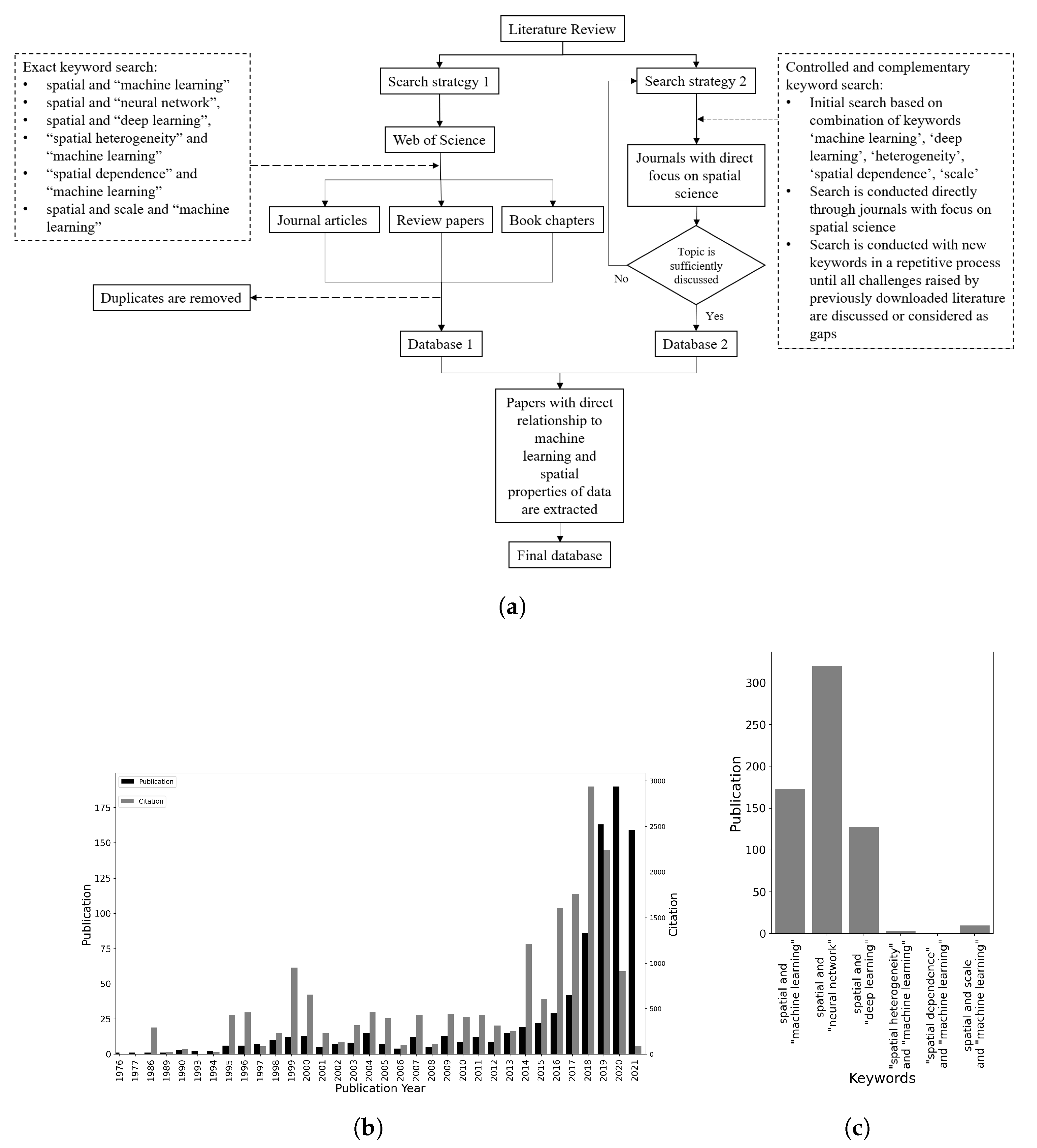
Figure 2.
Machine learning.

Figure 3.
Machine learning of spatial data.

Figure 4.
Anchorage regions (left) and containerized berth regions (right) outside and inside the port of Rotterdam. Points represent the vessel trajectory instances every hour. Point clusters may inform about the boundaries of each zone (bottom). In addition, the shape, the duration of visits, number of unique vessels, and vessel types within each region can inform its functionality.

Figure 5.
(a) Method proposed by [106] (reprinted with permission from Springer Nature: Springer, https://link.springer.com/chapter/10.1007/978-3-319-64689-3_8 Deep projective 3D semantic segmentation by Lawin, F.J.; Danelljan, M.; Tosteberg, P.; Bhat, G.; Khan, F.S.; Felsberg, M. COPYRIGHT (2017)). The 2D images are create by projecting the input point cloud into multiple virtual camera views. Semantic segmentation is conducted on for each view. The output prediction scores from all views are used to estimate a single prediction for each point. This process results in a 3D semantic segmentation of the point cloud. (b) The multi-scale representation of point clouds in [78] (https://www.tandfonline.com/doi/full/10.1080/13658816.2018.1552790 Using multi-scale and hierarchical deep convolutional features for 3D semantic classification of TLS point clouds. Guo, Z.; Feng, C.C. International Journal of Geographical Information Science 2020, 34, 661–680., Taylor and Francis. reprinted by permission of the publisher), with the finest scale1 at the bottom and the coarser scalel on the top).
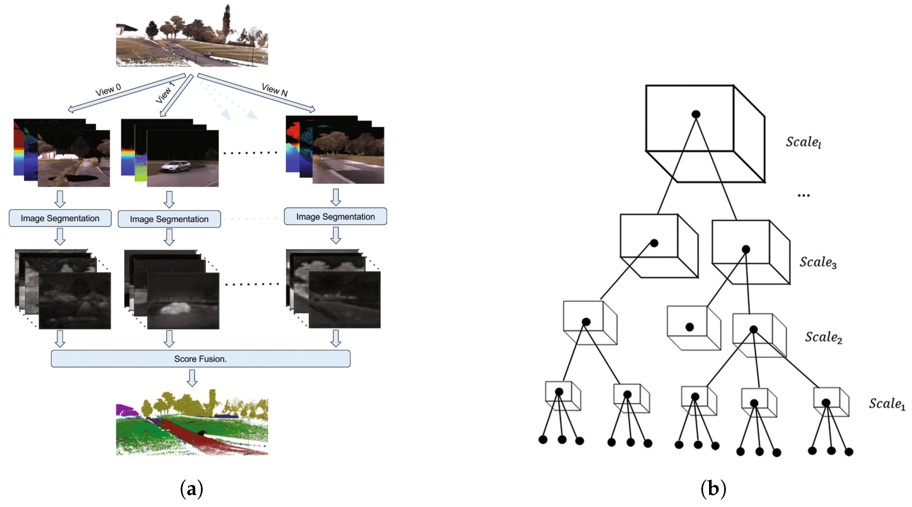
Figure 6.
Ref. [112] (https://www.tandfonline.com/doi/full/10.1080/13658816.2011.554838 Geographically weighted principal components analysis. Harris, P.; Brunsdon, C.; Charlton, M. International Journal of Geographical Information Science 2011, 25, 1717–1736, Taylor and Francis. Reprinted by permission of the publisher). (a) Summary of global PCA for eight variables representing social structure in Greater Dublin (the first three components express more than 70% of variations). (b) Spatial distribution of first component scores from global PCA.
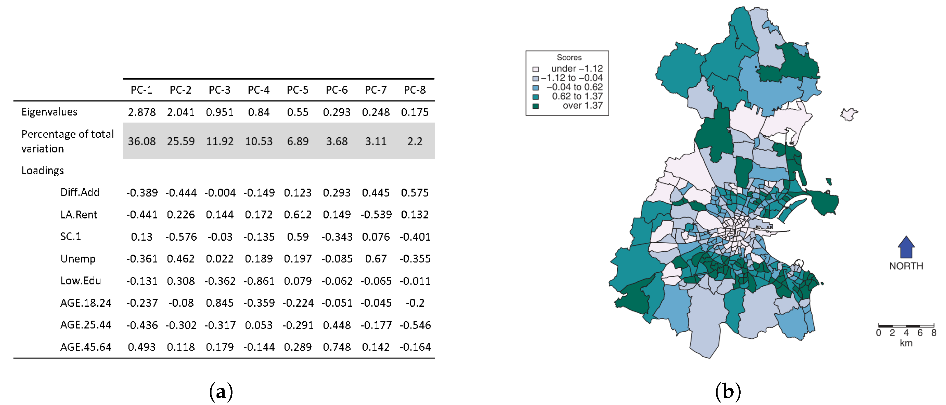
Figure 7.
Observations are transformed to a higher-dimensionality space (for simplicity, a 2D space). (a) Among all possible hyperplanes (line or curves in the current 2D example), the hyperplane that maximizes the margin Є is optimum (l1). (b) In practice, outliers exist in observations. While there is still a hyperplane that can separate the two classes, it may result in overfitting.

Figure 8.
(a) Reprinted from [128], Copyright (2013), with permission from Elsevier. The document map of nearly 7 million patent abstracts (background). Twenty best-matched nodes are marked for the query “laser surgery on the cornea” (blues circles within the enlarged map). (b) Reprinted from [130], Copyright (2017), with permission from Elsevier. One-dimensional SOM with 100 nodes, trained with a three-dimensional data set: the final weight vectors of the trained SOM are color-coded based on their index numbers from 1 to 100. (c) Reprinted from [130], Copyright (2017), with permission from Elsevier. Contextual map of London based on the average working hours, the average distance traveled to work, and the average age within each ward.
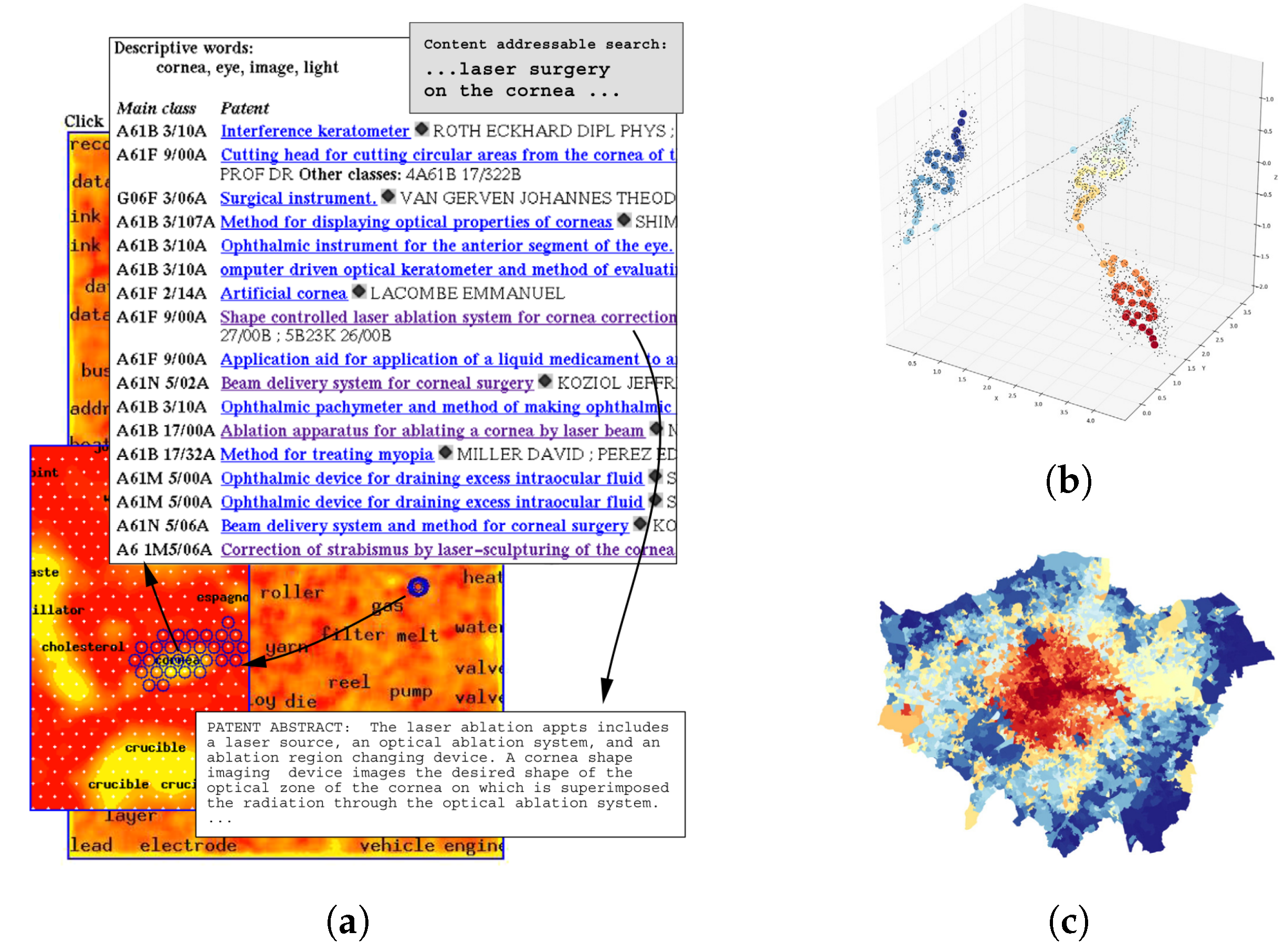
Figure 9.
Reprinted by permission from [140], Springer Nature Customer Service Centre GmbH: https://www.apress.com/us/book/9781484228449 Apress by Kim, P, Copyright (2017). (a) Basic structure of a CNN. (b) convolutional layer.
Figure 9.
Reprinted by permission from [140], Springer Nature Customer Service Centre GmbH: https://www.apress.com/us/book/9781484228449 Apress by Kim, P, Copyright (2017). (a) Basic structure of a CNN. (b) convolutional layer.
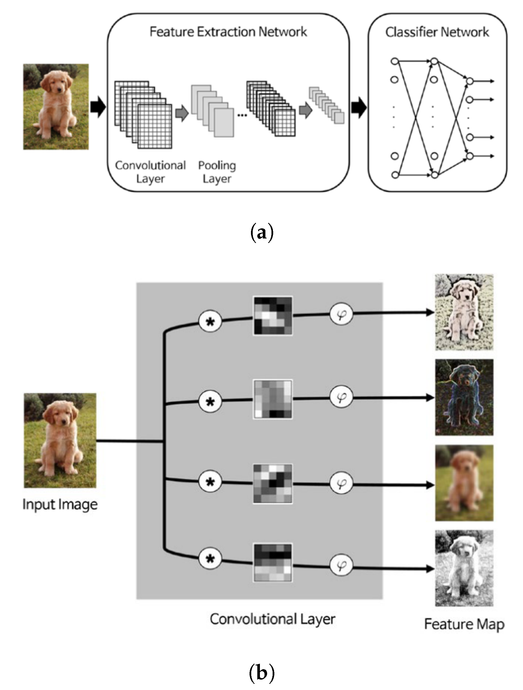
Figure 10.
The basic structure of two generative neural network models. (a) Variational autoencoders (VAE). (b) generative adversarial neural networks (GAN).
Figure 10.
The basic structure of two generative neural network models. (a) Variational autoencoders (VAE). (b) generative adversarial neural networks (GAN).
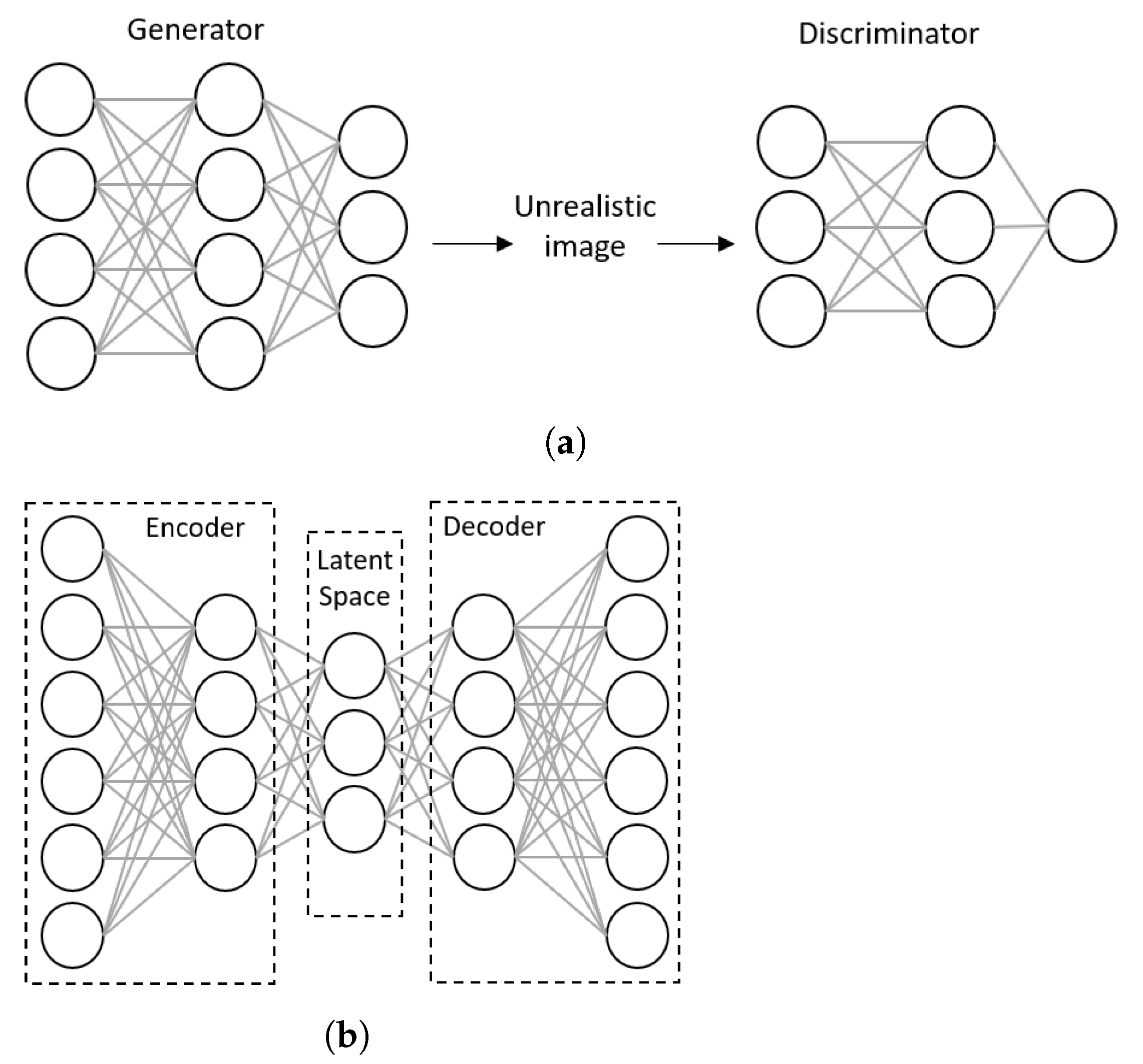
Figure 11.
Reprinted with permission from [180] (Copyright ©2001 Society for Industrial and Applied Mathematics. All rights reserved.) Spatial accuracy. (a) Actual location of nests, (b) Rasterized location of nests, (c) Predicted locations 1, (d) Predicted locations 2.
Figure 11.
Reprinted with permission from [180] (Copyright ©2001 Society for Industrial and Applied Mathematics. All rights reserved.) Spatial accuracy. (a) Actual location of nests, (b) Rasterized location of nests, (c) Predicted locations 1, (d) Predicted locations 2.
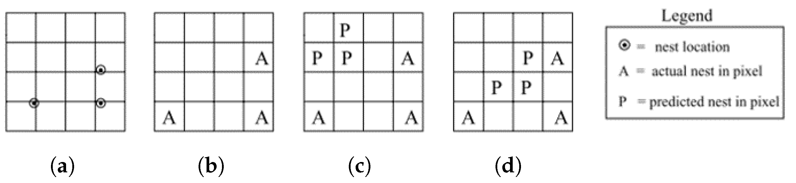
Figure 12.
Model complexity and regularization. (a) Overfitting: small lambda value. (b) Well-fitted: lambda value is tuned. (c) Underfitting: large lambda value.
Figure 12.
Model complexity and regularization. (a) Overfitting: small lambda value. (b) Well-fitted: lambda value is tuned. (c) Underfitting: large lambda value.
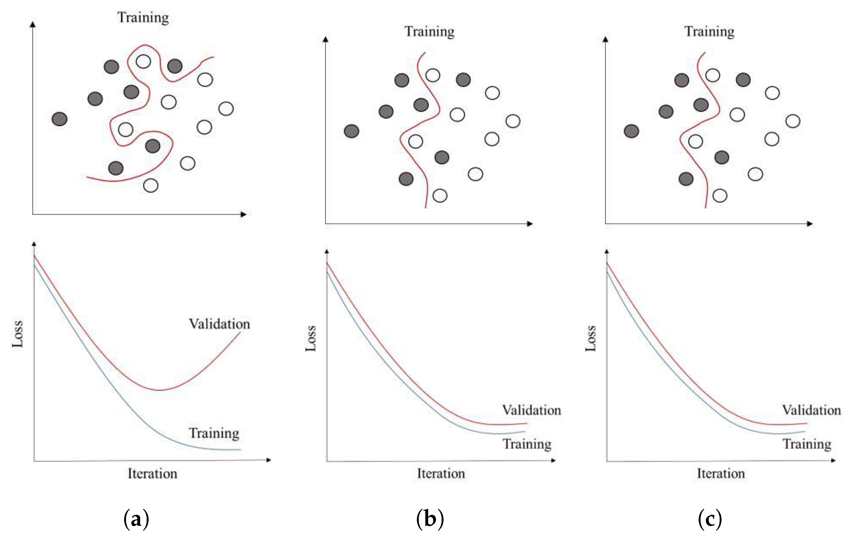
Publisher’s Note: MDPI stays neutral with regard to jurisdictional claims in published maps and institutional affiliations. |
© 2021 by the authors. Licensee MDPI, Basel, Switzerland. This article is an open access article distributed under the terms and conditions of the Creative Commons Attribution (CC BY) license (https://creativecommons.org/licenses/by/4.0/).
Share and Cite
MDPI and ACS Style
Nikparvar, B.; Thill, J.-C. Machine Learning of Spatial Data. ISPRS Int. J. Geo-Inf. 2021, 10, 600. https://doi.org/10.3390/ijgi10090600
AMA Style
Nikparvar B, Thill J-C. Machine Learning of Spatial Data. ISPRS International Journal of Geo-Information. 2021; 10(9):600. https://doi.org/10.3390/ijgi10090600
Chicago/Turabian StyleNikparvar, Behnam, and Jean-Claude Thill. 2021. "Machine Learning of Spatial Data" ISPRS International Journal of Geo-Information 10, no. 9: 600. https://doi.org/10.3390/ijgi10090600
Note that from the first issue of 2016, this journal uses article numbers instead of page numbers. See further details here.