
A Mechanistic Data-Driven Approach to Synthesize Human Mobility Considering the Spatial, Temporal, and Social Dimensions Together


Abstract
:1. Introduction
Open Source
2. Related Work
Position of Our Work
3. Definitions
3.1. Trajectory
3.2. Spatial Tessellation
3.3. Mobility Diary
3.4. Visitation Pattern
3.5. Contact Graph
3.6. Problem Definition
- A set of spatial (), temporal (), and social patterns (). The patterns refer to the distributions of mobility measures that quantify aspects related to the spatial, temporal, or social aspects of an individual’s mobility (e.g., radius of gyration, mobility entropy, mobility similarity). A realistic is expected to reproduce as many mobility patterns as possible.
- A set of real mobility trajectories corresponding to m real individuals that move on the same region as the one on which synthetic trajectories are generated. is used to compute the set of patterns, which are compared with the patterns computed on .
- A function D that computes the dissimilarity between two distributions. Specifically, for each measure in , indicates the dissimilarity between , the distribution of the measures computed on the synthetic trajectories in , and , the distribution of the measures computed on the real trajectories in . The lower , the more realistic model M is with respect to f and .
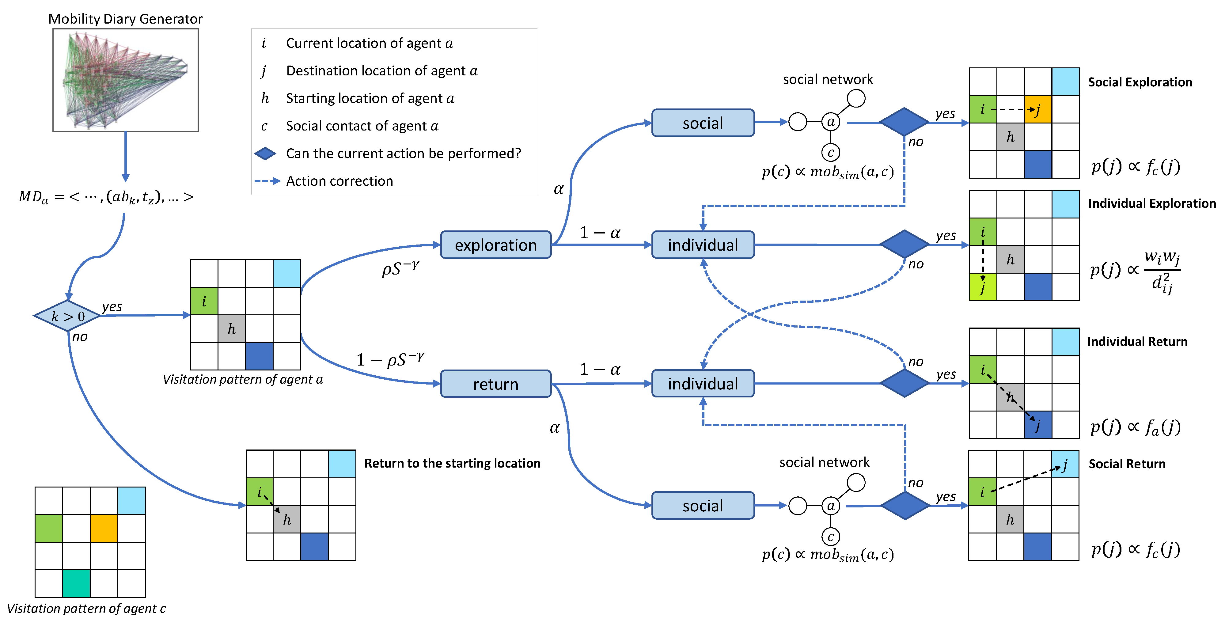
4. The STS-EPR Model
4.1. Initialization
4.2. Action Selection
4.3. Location Selection
- Individual Exploration (IE): a chooses a new location to explore from . Individuals are more likely to move at small rather than long distances but also take into account the location’s collective relevance [31]. We use the gravity law to couple distance and relevance [37]. If a is currently at location , it selects an unvisited location , with , with probability , where is the geographic distance between locations and with relevances , .
- Social Exploration (SE): a selects an agent c among its social contacts in the social graph G, i.e., . The probability for c to be selected is proportional to the mobility-similarity between them: . After the contact c is chosen, the candidate location to explore is an unvisited location for a that was visited by c, i.e., the location is selected from set . The probability for a location , with , to be selected is proportional to the visitation pattern of c, namely .
- Individual Return (IR): a chooses the return location from the set with a probability proportional to its visitation pattern. The probability for a location with to be chosen is: .
- Social Return (SR):c is selected as in SE, and the location a returns to is picked from the set . The probability for a location to be selected is proportional to the visitation pattern of the agent c, namely .
4.4. Action Correction
- No location in social choices: If an agent a decides to move with the influence of a social contact c, but or (no locations visited by both c and a or no locations visited by c and unvisited by a), we execute an individual action preserving a’s choice to explore or return.
- No new location to explore: When an agent a decides to explore but it visited all the locations at least once (), we force the agent to make an IR action.
- No return location: If an agent a, currently at location , decides to perform an IR, and is the only location visited so far (besides the starting location), it cannot return to any location (). We force a to make an IE.
5. Experiments
5.1. Datasets
5.1.1. Trajectories Dataset
5.1.2. Social Graph
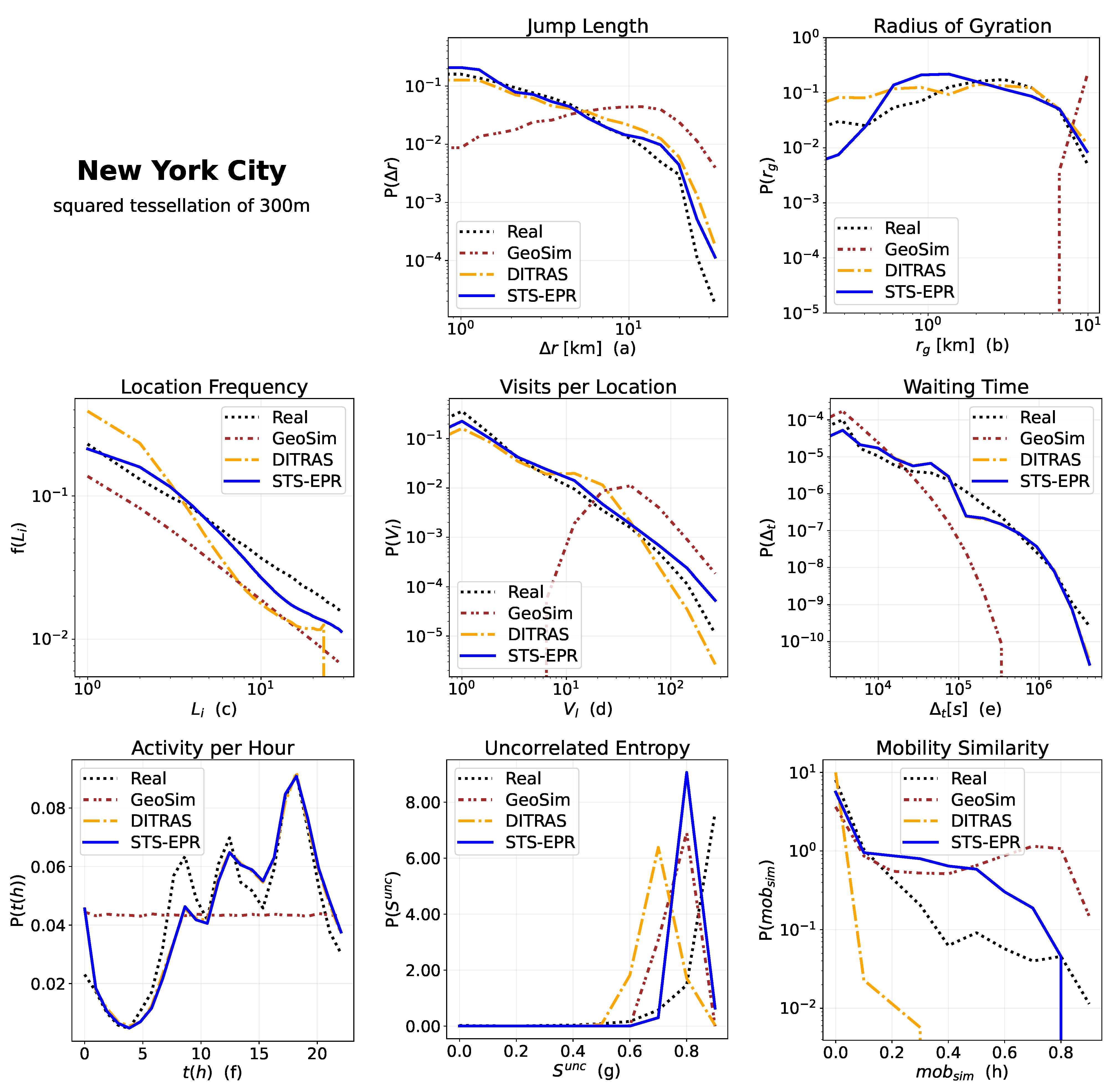
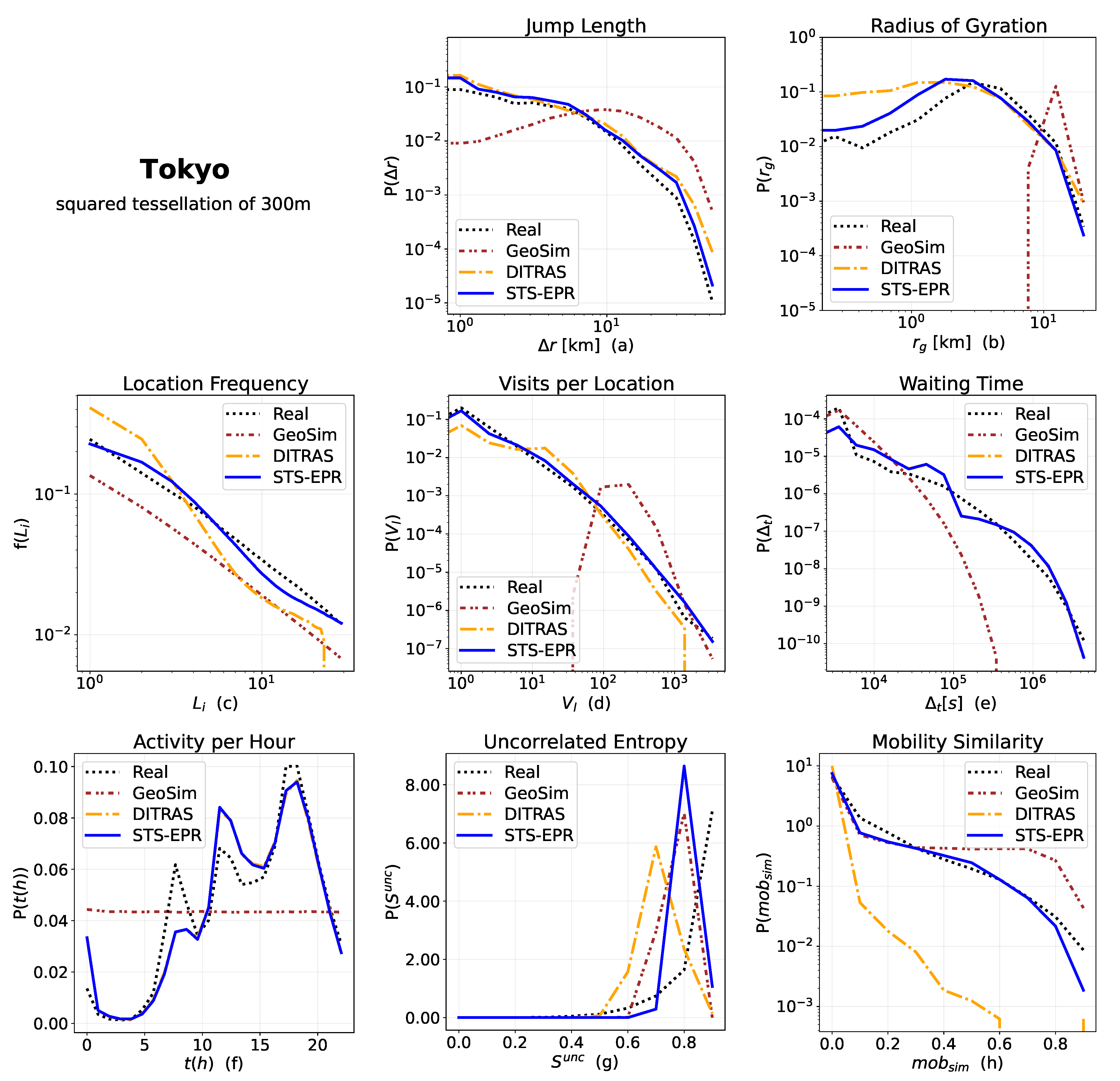
5.2. Measures
- Jump Length , the distance between two consecutive locations visited by an individual [28,29,30]. Formally, is the geographical distance between two points and in a trajectory. A truncated power-law well approximates the empirical distribution within a population of individuals, with the value of the exponent slightly varying based on the type of data and the spatial scale [28,29].
- Radius of Gyration , the typical distance travelled by an individual u during the period of observation [29,35]. The of individual u defined as , where is the number of points in , and is the position vector of the centre of mass of the set of points in . A truncated power-law well approximates the distribution of [29,30].
- Location Frequency , the probability of an individual to visit a location [29], identifying the importance of a location to an individual’s mobility: the most visited location (likely home or work) has rank 1, the second most visited location (e.g., school or local shop) has rank 2, and so on. The probability of finding an individual at a location of rank L is well approximated by [29,30].
- Waiting Time : the elapsed time between two consecutive visits of an individual u: . Empirically the distribution of waiting times is well approximated by a truncated power-law [34].
- Activity per Hour : the number of movements made by the individuals at every hour of the day [31,40]. The movements of individuals are not distributed uniformly during the hours of the day but follow a circadian rhythm: people tend to be stationary during the night hours while prefer moving at specific times of the day, for example, to reach the workplace or return home.
- We define the mobility similarity between two individuals as the cosine-similarity of their location vectors .
5.3. Experimental Settings
6. Results
6.1. Spatial
6.2. Temporal
6.3. Social
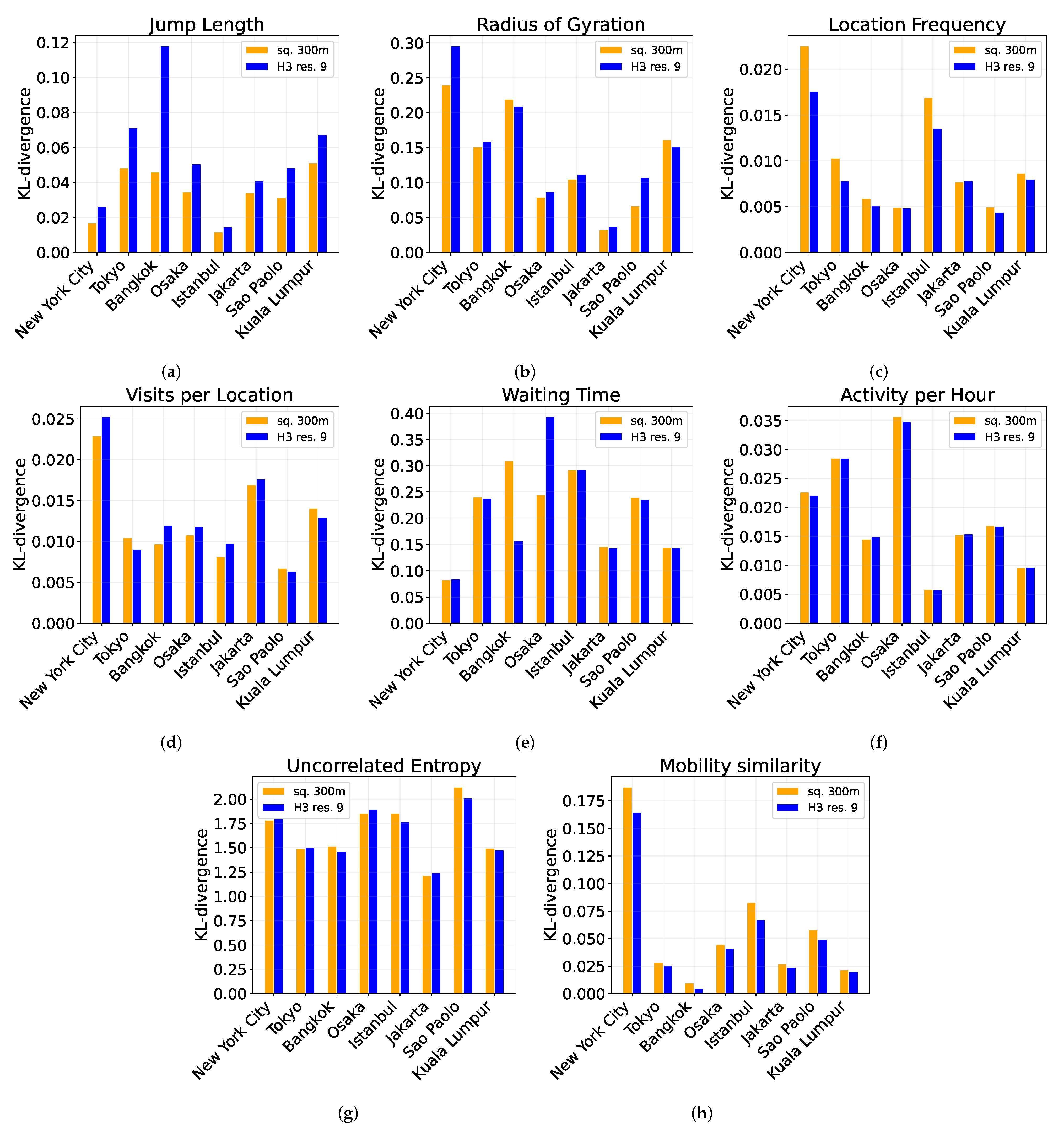
6.4. Impact of Spatial Tessellation
- Squared tessellation with tiles of size 300 m and area 0.09 km;
- Hexagonal tessellation with tiles of H3 resolution 9 and area 0.10 km;
6.5. Discussion
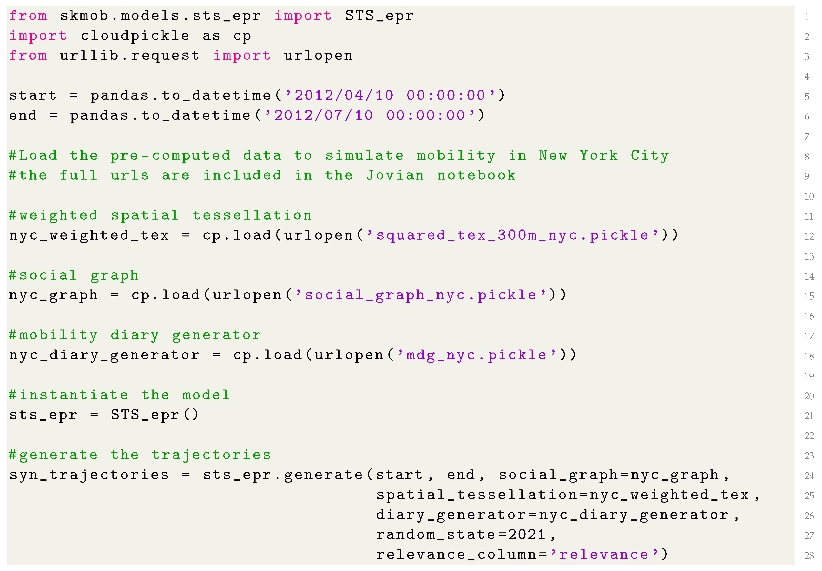
7. Example of Execution
| Listing 1: STS-EPR Python example. |
 |
8. Conclusions
Supplementary Materials
Author Contributions
Funding
Data Availability Statement
Acknowledgments
Conflicts of Interest
References
- Pepe, E.; Bajardi, P.; Gauvin, L.; Privitera, F.; Lake, B.; Cattuto, C.; Tizzoni, M. COVID-19 outbreak response, a dataset to assess mobility changes in Italy following national lockdown. Sci. Data 2020, 7, 1–7. [Google Scholar] [CrossRef] [PubMed]
- Kraemer, M.U.; Yang, C.H.; Gutierrez, B.; Wu, C.H.; Klein, B.; Pigott, D.M.; Du Plessis, L.; Faria, N.R.; Li, R.; Hanage, W.P.; et al. The effect of human mobility and control measures on the COVID-19 epidemic in China. Science 2020, 368, 493–497. [Google Scholar] [CrossRef] [PubMed] [Green Version]
- Oliver, N.; Lepri, B.; Sterly, H.; Lambiotte, R.; Deletaille, S.; De Nadai, M.; Letouzé, E.; Salah, A.A.; Benjamins, R.; Cattuto, C.; et al. Mobile phone data for informing public health actions across the COVID-19 pandemic life cycle. Sci. Adv. 2020, 6, eabc0764. [Google Scholar] [CrossRef]
- Andrienko, G.; Andrienko, N.; Boldrini, C.; Caldarelli, G.; Cintia, P.; Cresci, S.; Facchini, A.; Giannotti, F.; Gionis, A.; Guidotti, R.; et al. (So) Big Data and the transformation of the city. Int. J. Data Sci. Anal. 2021, 11, 311–340. [Google Scholar] [CrossRef] [Green Version]
- Huang, X.; Li, Z.; Jiang, Y.; Ye, X.; Deng, C.; Zhang, J.; Li, X. The characteristics of multi-source mobility datasets and how they reveal the luxury nature of social distancing in the U.S. during the COVID-19 pandemic. Int. J. Digit. Earth 2021, 14, 424–442. [Google Scholar] [CrossRef]
- Rossi, A.; Barlacchi, G.; Bianchini, M.; Lepri, B. Modelling Taxi Drivers’ Behaviour for the Next Destination Prediction. IEEE Trans. Intell. Transp. Syst. 2019, 21, 2980–2989. [Google Scholar] [CrossRef]
- Khaidem, L.; Luca, M.; Yang, F.; Anand, A.; Lepri, B.; Dong, W. Optimizing Transportation Dynamics at a City-Scale Using a Reinforcement Learning Framework. IEEE Access 2020, 8, 171528–171541. [Google Scholar] [CrossRef]
- Pappalardo, L.; Ferres, L.; Sacasa, M.; Cattuto, C.; Bravo, L. Evaluation of home detection algorithms on mobile phone data using individual-level ground truth. EPJ Data Sci. 2021, 10, 29. [Google Scholar] [CrossRef] [PubMed]
- Deville, P.; Linard, C.; Martin, S.; Gilbert, M.; Stevens, F.R.; Gaughan, A.E.; Blondel, V.D.; Tatem, A.J. Dynamic population mapping using mobile phone data. Proc. Natl. Acad. Sci. USA 2014, 111, 15888–15893. [Google Scholar] [CrossRef] [Green Version]
- Sîrbu, A.; Andrienko, G.; Andrienko, N.; Boldrini, C.; Conti, M.; Giannotti, F.; Guidotti, R.; Bertoli, S.; Kim, J.; Muntean, C.I.; et al. Human migration: The big data perspective. Int. J. Data Sci. Anal. 2020, 11, 341–360. [Google Scholar] [CrossRef]
- Bohm, M.; Nanni, M.; Pappalardo, L. Quantifying the presence of air pollutants over a road network in high spatio-temporal resolution. In Proceedings of the NeurIPS 2021 Workshop—Tackling Climate Change with Machine Learning, Online, 13–14 December 2020. [Google Scholar]
- Nyhan, M.; Kloog, I.; Britter, R.; Ratti, C.; Koutrakis, P. Quantifying population exposure to air pollution using individual mobility patterns inferred from mobile phone data. J. Expo. Sci. Environ. Epidemiol. 2019, 29, 238–247. [Google Scholar] [CrossRef]
- Pappalardo, L.; Vanhoof, M.; Gabrielli, L.; Smoreda, Z.; Pedreschi, D.; Giannotti, F. An analytical framework to nowcast well-being using mobile phone data. Int. J. Data Sci. Anal. 2016, 2, 75–92. [Google Scholar] [CrossRef] [Green Version]
- Voukelatou, V.; Gabrielli, L.; Miliou, I.; Cresci, S.; Sharma, R.; Tesconi, M.; Pappalardo, L. Measuring objective and subjective well-being: Dimensions and data sources. Int. J. Data Sci. Anal. 2020, 11, 279–309. [Google Scholar] [CrossRef]
- Newlands, G.; Lutz, C.; Tamò-Larrieux, A.; Villaronga, E.F.; Harasgama, R.; Scheitlin, G. Innovation under pressure: Implications for data privacy during the Covid-19 pandemic. Big Data Soc. 2020, 7, 2053951720976680. [Google Scholar] [CrossRef]
- Montjoye, Y.A.; Hidalgo, C.; Verleysen, M.; Blondel, V. Unique in the Crowd: The Privacy Bounds of Human Mobility. Sci. Rep. 2013, 3, 1376. [Google Scholar] [CrossRef] [Green Version]
- Montjoye, Y.A.; Gambs, S.; Blondel, V.; Canright, G.; Cordes, N.; Deletaille, S.; Engø-Monsen, K.; García-Herranz, M.; Kendall, J.; Kerry, C.; et al. On the privacy-conscientious use of mobile phone data. Sci. Data 2018, 5, 180286. [Google Scholar] [CrossRef]
- Pellungrini, R.; Pappalardo, L.; Pratesi, F.; Monreale, A. A Data Mining Approach to Assess Privacy Risk in Human Mobility Data. ACM Trans. Intell. Syst. Technol. 2017, 9, 31:1–31:27. [Google Scholar] [CrossRef] [Green Version]
- Pellungrini, R.; Pappalardo, L.; Simini, F.; Monreale, A. Modeling Adversarial Behavior Against Mobility Data Privacy. IEEE Trans. Intell. Transp. Syst. 2020. [Google Scholar] [CrossRef]
- Mir, D.J.; Isaacman, S.; Cáceres, R.; Martonosi, M.; Wright, R.N. DP-WHERE: Differentially private modeling of human mobility. In Proceedings of the 2013 IEEE International Conference on Big Data, Silicon Valley, CA, USA, 6–9 October 2013; pp. 580–588. [Google Scholar]
- Fiore, M.; Katsikouli, P.; Zavou, E.; Cunche, M.; Fessant, F.; Hello, D.L.; Aivodji, U.M.; Olivier, B.; Quertier, T.; Stanica, R. Privacy in trajectory micro-data publishing: A survey. arXiv 2019, arXiv:1903.12211. [Google Scholar]
- Barbosa-Filho, H.; Barthelemy, M.; Ghoshal, G.; James, C.; Lenormand, M.; Louail, T.; Menezes, R.; Ramasco, J.J.; Simini, F.; Tomasini, M. Human mobility: Models and applications. Phys. Rep. 2018, 734, 1–74. [Google Scholar] [CrossRef] [Green Version]
- Luca, M.; Barlacchi, G.; Lepri, B.; Pappalardo, L. A Survey on Deep Learning for Human Mobility. arXiv 2021, arXiv:2012.02825. [Google Scholar]
- Karamshuk, D.; Boldrini, C.; Conti, M.; Passarella, A. Human mobility models for opportunistic networks. IEEE Commun. Mag. 2011, 49, 157–165. [Google Scholar] [CrossRef]
- Solmaz, G.; Turgut, D. A Survey of Human Mobility Models. IEEE Access 2019, 7, 125711–125731. [Google Scholar] [CrossRef]
- Hess, A.; Hummel, K.A.; Gansterer, W.N.; Haring, G. Data-driven human mobility modeling: A survey and engineering guidance for mobile networking. ACM Comput. Surv. (CSUR) 2015, 48, 1–39. [Google Scholar] [CrossRef]
- Tomasini, M.; Mahmood, B.; Zambonelli, F.; Brayner, A.; Menezes, R. On the effect of human mobility to the design of metropolitan mobile opportunistic networks of sensors. Pervasive Mob. Comput. 2017, 38, 215–232. [Google Scholar] [CrossRef] [Green Version]
- Brockmann, D.; Hufnagel, L.; Geisel, T. The Scaling Laws of Human Travel. Nature 2006, 439, 462–465. [Google Scholar] [CrossRef]
- Gonzalez, M.C.; Hidalgo, C.; Barabasi, A.L. Understanding Individual Human Mobility Patterns. Nature 2008, 453, 779–782. [Google Scholar] [CrossRef]
- Pappalardo, L.; Rinzivillo, S.; Qu, Z.; Pedreschi, D.; Giannotti, F. Understanding the patterns of car travel. Eur. Phys. J. Spec. Top. 2013, 215, 61–73. [Google Scholar] [CrossRef]
- Pappalardo, L.; Simini, F. Data-driven generation of spatio-temporal routines in human mobility. Data Min. Knowl. Discov. 2017, 32. [Google Scholar] [CrossRef] [Green Version]
- Cho, E.; Myers, S.; Leskovec, J. Friendship and Mobility: User Movement In Location-Based Social Networks. In Proceedings of the 17th ACM SIGKDD International Conference on Knowledge Discovery and Data Mining, San Diego, CA, USA, 21–24 August 2011; pp. 1082–1090. [Google Scholar] [CrossRef]
- Toole, J.; Herrera-Yague, C.; Schneider, C.; Gonzalez, M.C. Coupling Human Mobility and Social Ties. J. R. Soc. Interface/R. Soc. 2015, 12. [Google Scholar] [CrossRef] [Green Version]
- Song, C.; Koren, T.; Wang, P.; Barabasi, A.L. Modelling the scaling properties of human mobility. Nat. Phys. 2010, 6, 818–823. [Google Scholar] [CrossRef] [Green Version]
- Pappalardo, L.; Simini, F.; Rinzivillo, S.; Pedreschi, D.; Giannotti, F.; Barabasi, A.L. Returners and explorers dichotomy in human mobility. Nat. Commun. 2015, 6, 8166. [Google Scholar] [CrossRef] [PubMed] [Green Version]
- Song, C.; Qu, Z.; Blumm, N.; Barabasi, A.L. Limits of Predictability in Human Mobility. Sciences 2010, 327, 1018–1021. [Google Scholar] [CrossRef] [PubMed] [Green Version]
- Pappalardo, L.; Rinzivillo, S.; Simini, F. Human Mobility Modelling: Exploration and Preferential Return Meet the Gravity Model. Procedia Comput. Sci. 2016, 83, 934–939. [Google Scholar] [CrossRef] [Green Version]
- Barbosa, H.; de Lima-Neto, F.B.; Evsukoff, A.; Menezes, R. The effect of recency to human mobility. EPJ Data Sci. 2015, 4, 21. [Google Scholar] [CrossRef] [Green Version]
- Alessandretti, L.; Sapiezynski, P.; Lehmann, S.; Baronchelli, A. Evidence for a Conserved Quantity in Human Mobility. Nat. Hum. Behav. 2018, 2, 485–491. [Google Scholar] [CrossRef]
- Jiang, S.; Yang, Y.; Gupta, S.; Veneziano, D.; Athavale, S.; Gonzalez, M.C. The TimeGeo modeling framework for urban mobility without travel surveys. Proc. Natl. Acad. Sci. USA 2016, 113, E5370–E5378. [Google Scholar] [CrossRef] [Green Version]
- Zheng, Y.; Capra, L.; Wolfson, O.; Yang, H. Urban computing: Concepts, methodologies, and applications. ACM Trans. Intell. Syst. Technol. (TIST) 2014, 5, 1–55. [Google Scholar] [CrossRef]
- Zheng, Y. Trajectory data mining: An overview. ACM Trans. Intell. Syst. Technol. (TIST) 2015, 6, 29. [Google Scholar] [CrossRef]
- Yang, D.; Qu, B.; Yang, J.; Cudre-Mauroux, P. Revisiting User Mobility and Social Relationships in LBSNs: A Hypergraph Embedding Approach. In Proceedings of the 2019World WideWeb Conference (WWW ’19), San Francisco, CA, USA, 13–17 May 2019; pp. 2147–2157. [Google Scholar] [CrossRef] [Green Version]
- Pappalardo, L.; Barlacchi, G.; Simini, F.; Pellungrini, R. Scikit-mobility: A Python library for the analysis, generation and risk assessment of mobility data. arXiv 2019, arXiv:1907.07062. [Google Scholar]
- Ouyang, K.; Shokri, R.; Rosenblum, D.S.; Yang, W. A Non-Parametric Generative Model for Human Trajectories. In Proceedings of the Twenty-Seventh International Joint Conference on Artificial Intelligence (IJCAI-18), Stockholm, Sweden, 13–19 July 2018; pp. 3812–3817. [Google Scholar]
- Eagle, N.; Pentland, A.S. Eigenbehaviors: Identifying structure in routine. Behav. Ecol. Sociobiol. 2009, 63, 1057–1066. [Google Scholar] [CrossRef] [Green Version]
- Wang, D.; Pedreschi, D.; Song, C.; Giannotti, F.; Barabasi, A.L. Human mobility, social ties, and link prediction. In Proceedings of the ACM SIGKDD International Conference on Knowledge Discovery and Data Mining, San Diego, CA, USA, 21–24 August 2011; pp. 1100–1108. [Google Scholar] [CrossRef]
- Fan, C.; Liu, Y.; Huang, J.; Rong, Z.; Zhou, T. Correlation between social proximity and mobility similarity. Sci. Rep. 2016, 7, 11975. [Google Scholar] [CrossRef] [PubMed] [Green Version]


| Parameter | Default Value | Is the Parameter Fitted from a Dataset? | It Models |
|---|---|---|---|
| 0.6 | no | explore or return choice | |
| 0.21 | no | explore or return choice | |
| 0.2 | no | social factor | |
| - | yes | relevances of the locations | |
| Mobility Diary Generator (MDG) | - | yes | mobility diary of agents |
| (a) | ||||
| user_id | location_id | UTC time | timezone | |
| ⋮ | ⋮ | ⋮ | ⋮ | |
| 268846 | 42872fd9b60caeb | Tue Apr 03 18:27:37 2012 | −240 | |
| 377500 | 3c38c65be1b8c04 | Tue Apr 03 18:27:38 2012 | −240 | |
| 248657 | 1855f964a520be3 | Tue Apr 03 18:27:38 2012 | −240 | |
| ⋮ | ⋮ | ⋮ | ⋮ | |
| (b) | ||||
| location_id | latitude | longitude | category | cc |
| ⋮ | ⋮ | ⋮ | ⋮ | ⋮ |
| 42872fd9b60caeb | 41.660393 | −83.615227 | College Cafeteria | US |
| 6200f964a520ee3 | 40.722206 | −73.981720 | Theater | US |
| 9cadf964a521fe3 | 44.972814 | −93.235313 | Student Center | US |
| ⋮ | ⋮ | ⋮ | ⋮ | ⋮ |
| Validation | Calibration | |||||
|---|---|---|---|---|---|---|
| City | #checkins | #users | #edges | avg. degree | #checkins | #users |
| New York City (US) | 37,489 | 1001 | 1755 | 3.506 | 247,058 | 19,416 |
| Osaka (JP) | 46,755 | 823 | 1734 | 4.214 | 48,832 | 3534 |
| Kuala Lumpur (MY) | 78,037 | 2582 | 5715 | 4.427 | 159,514 | 13,453 |
| Sao Paulo (BR) | 86,654 | 1651 | 3725 | 4.512 | 266,235 | 15,733 |
| Jakarta (ID) | 99,460 | 2162 | 3781 | 3.498 | 391,576 | 35,576 |
| Bangkok (TH) | 109,585 | 2044 | 5228 | 5.115 | 265,670 | 15,632 |
| Istanbul (TR) | 228,755 | 5089 | 9918 | 3.898 | 555,913 | 33,454 |
| Tokyo (JP) | 229,283 | 4043 | 16,137 | 7.983 | 185,809 | 12,825 |
| New York City | STS-EPR | 0.017 ±0.0012 | 0.2399 ±0.0797 | 0.0225 ±0.0006 | 0.0229 ±0.0044 | 0.0827 ±0.0006 | 0.0227 ±0.0012 | 1.7856 ±0.0688 | 0.1874 ±0.006 |
| DITRAS | 0.0199 ±0.0021 | 0.0848 ±0.0162 | 0.1505 ±0.0052 | 0.077 ±0.0059 | 0.0848 ±0.0015 | 0.0233 ±0.0008 | 3.3201 ±0.3192 | 0.7903 ±0.1218 | |
| GeoSim | 0.7906 ±0.0034 | 5.3613 ±0.0193 | 0.0049 ±0.0004 | 4.4898 ±0.0154 | 0.9752 ±0.0464 | 0.1801 ±0.0006 | 7.997 ±0.0771 | 0.5558 ±0.0116 | |
| Tokyo | STS-EPR | 0.0485 ±0.0024 | 0.1517 ±0.0133 | 0.0103 ±0.0003 | 0.0105 ±0.0006 | 0.2406 ±0.0012 | 0.0285 ±0.0004 | 1.4906 ±0.0166 | 0.0284 ±0.0025 |
| DITRAS | 0.066 ±0.0013 | 0.3905 ±0.0183 | 0.1132 ±0.0011 | 0.1201 ±0.009 | 0.2398 ±0.0024 | 0.0286 ±0.0006 | 2.1747 ±0.2988 | 1.0454 ±0.0369 | |
| GeoSim | 0.7402 ±0.0032 | 4.8877 ±0.0058 | 0.0001 ±0.0 | 2.9007 ±0.0067 | 1.0047 ±0.0004 | 0.2874 ±0.0001 | 6.658 ±0.0238 | 0.098 ±0.0023 | |
| Bangkok | STS-EPR | 0.046 ±0.0016 | 0.2195 ±0.1916 | 0.0059 ±0.0059 | 0.0097 ±0.001 | 0.3094 ±0.1848 | 0.0145 ±0.0003 | 1.5182 ±0.0574 | 0.0099 ±0.0023 |
| DITRAS | 0.0336 ±0.0027 | 0.1992 ±0.0089 | 0.0893 ±0.0021 | 0.0663 ±0.0042 | 0.1578 ±0.0007 | 0.0147 ±0.0004 | 2.1252 ±0.0341 | 1.5523 ±0.105 | |
| GeoSim | 0.7391 ±0.003 | 5.1465 ±0.005 | 0.0023 ±0.0002 | 3.6032 ±0.0031 | 0.9575 ±0.0002 | 0.2928 ±0.0004 | 4.8474 ±0.0982 | 0.1742 ±0.003 | |
| Osaka | STS-EPR | 0.0346 ±0.0041 | 0.0793 ±0.0096 | 0.0049 ±0.0001 | 0.0108 ±0.0019 | 0.2447 ±0.0033 | 0.0357 ±0.0007 | 1.8577 ±0.0439 | 0.0449 ±0.0045 |
| DITRAS | 0.0625 ±0.009 | 0.125 ±0.0154 | - - | 0.0566 ±0.0032 | 0.2474 ±0.0032 | 0.0362 ±0.0003 | 2.3668 ±0.0676 | 1.2222 ±0.0659 | |
| GeoSim | 0.7792 ±0.0061 | 5.0454 ±0.0048 | 0.0037 ±0.0002 | 4.079 ±0.0112 | 1.0225 ±0.0009 | 0.3062 ±0.0004 | 7.1387 ±0.0007 | 0.3126 ±0.0142 | |
| Istanbul | STS-EPR | 0.0118 ±0.0009 | 0.1051 ±0.0243 | 0.0169 ±0.0002 | 0.0082 ±0.0007 | 0.2924 ±0.1858 | 0.0059 ±0.0002 | 1.8559 ±0.0488 | 0.0828 ±0.0009 |
| DITRAS | 0.0242 ±0.0016 | 0.8151 ±0.0133 | 0.1381 ±0.0009 | 0.1096 ±0.0049 | 0.2164 ±0.186 | 0.0057 ±0.0001 | 3.5716 ±0.1668 | 1.0926 ±0.0422 | |
| GeoSim | 0.5296 ±0.0021 | 4.9211 ±0.0005 | 0.0012 ±0.0001 | 2.8892 ±0.0021 | 0.9735 ±0.047 | 0.2228 ±0.0002 | 6.0196 ±0.0104 | 0.3583 ±0.0056 | |
| Jakarta | STS-EPR | 0.0341 ±0.0023 | 0.0329 ±0.006 | 0.0077 ±0.0002 | 0.017 ±0.0023 | 0.1466 ±0.0037 | 0.0153 ±0.0003 | 1.2139 ±0.027 | 0.0269 ±0.0044 |
| DITRAS | 0.0203 ±0.0012 | 0.2938 ±0.0221 | 0.0683 ±0.0 | 0.1003 ±0.0028 | 0.1443 ±0.0014 | 0.0157 ±0.0005 | 1.1002 ±0.054 | 1.8143 ±0.1379 | |
| GeoSim | 0.7069 ±0.0031 | 5.3784 ±0.0046 | 0.0038 ±0.0004 | 3.4635 ±0.0031 | 0.9631 ±0.0002 | 0.2198 ±0.0003 | 5.1984 ±0.1167 | 0.3275 ±0.0065 | |
| Sao Paulo | STS-EPR | 0.0314 ±0.0015 | 0.0669 ±0.0169 | 0.005 ±0.0002 | 0.0067 ±0.0006 | 0.2394 ±0.1604 | 0.0169 ±0.0007 | 2.123 ±0.0837 | 0.0582 ±0.0026 |
| DITRAS | 0.0212 ±0.001 | 0.1949 ±0.0149 | 0.0741 ±0.0007 | 0.0448 ±0.0035 | 0.2386 ±0.1601 | 0.0165 ±0.0004 | 2.1078 ±0.0572 | 0.7835 ±0.049 | |
| GeoSim | 0.6968 ±0.0032 | 5.8012 ±0.0387 | 0.0072 ±0.0004 | 3.8986 ±0.0289 | 0.9886 ±0.0002 | 0.1692 ±0.0003 | 5.2005 ±0.1224 | 0.3532 ±0.0062 | |
| Kuala Lumpur | STS-EPR | 0.0513 ±0.0015 | 0.1616 ±0.0068 | 0.0087 ±0.0002 | 0.0141 ±0.0048 | 0.1448 ±0.0017 | 0.0096 ±0.0001 | 1.4955 ±0.027 | 0.0217 ±0.0072 |
| DITRAS | 0.0442 ±0.0047 | 0.6756 ±0.0265 | - - | 0.2834 ±0.0203 | 0.1452 ±0.0021 | 0.0097 ±0.0002 | 1.723 ±0.0369 | 1.0451 ±0.0626 | |
| GeoSim | 0.6494 ±0.0006 | 4.6041 ±0.0153 | 0.0025 ±0.0001 | 2.188 ±0.0045 | 0.978 ±0.0002 | 0.192 ±0.0005 | 6.7618 ±0.0996 | 0.2336 ±0.0044 |
| # Relevant Tiles | ||
|---|---|---|
| City | sq. 300 m | hex. H3 res 9 |
| New York City (US) | 6734 | 4498 |
| Osaka (JP) | 3690 | 3270 |
| Kuala Lumpur (MY) | 2221 | 1691 |
| Sao Paulo (BR) | 6962 | 5588 |
| Jakarta (ID) | 6160 | 5215 |
| Bangkok (TH) | 7016 | 5518 |
| Istanbul (TR) | 8976 | 5265 |
| Tokyo (JP) | 7417 | 5844 |
Publisher’s Note: MDPI stays neutral with regard to jurisdictional claims in published maps and institutional affiliations. |
© 2021 by the authors. Licensee MDPI, Basel, Switzerland. This article is an open access article distributed under the terms and conditions of the Creative Commons Attribution (CC BY) license (https://creativecommons.org/licenses/by/4.0/).
Share and Cite
Cornacchia, G.; Pappalardo, L. A Mechanistic Data-Driven Approach to Synthesize Human Mobility Considering the Spatial, Temporal, and Social Dimensions Together. ISPRS Int. J. Geo-Inf. 2021, 10, 599. https://doi.org/10.3390/ijgi10090599
Cornacchia G, Pappalardo L. A Mechanistic Data-Driven Approach to Synthesize Human Mobility Considering the Spatial, Temporal, and Social Dimensions Together. ISPRS International Journal of Geo-Information. 2021; 10(9):599. https://doi.org/10.3390/ijgi10090599
Chicago/Turabian StyleCornacchia, Giuliano, and Luca Pappalardo. 2021. "A Mechanistic Data-Driven Approach to Synthesize Human Mobility Considering the Spatial, Temporal, and Social Dimensions Together" ISPRS International Journal of Geo-Information 10, no. 9: 599. https://doi.org/10.3390/ijgi10090599