Article

A Unifying Framework for Analysis of Spatial-Temporal Event Sequence Similarity and Its Applications

School of Computing and Information Science, University of Maine, Orono, ME 04469, USA
*
Author to whom correspondence should be addressed.
ISPRS Int. J. Geo-Inf. 2021, 10(9), 594; https://doi.org/10.3390/ijgi10090594
Submission received: 27 June 2021 / Revised: 26 August 2021 / Accepted: 5 September 2021 / Published: 9 September 2021
(This article belongs to the Special Issue Spatio-Temporal Models and Geo-Technologies)

Abstract

:
Measures of similarity or differences between data objects are applied frequently in geography, biology, computer science, linguistics, logic, business analytics, and statistics, among other fields. This work focuses on event sequence similarity among event sequences extracted from time series observed at spatially deployed monitoring locations with the aim of enhancing the understanding of process similarity over time and geospatial locations. We present a framework for a novel matrix-based spatiotemporal event sequence representation that unifies punctual and interval-based representation of events. This unified representation of spatiotemporal event sequences (STES) supports different event data types and provides support for data mining and sequence classification and clustering. The similarity measure is based on the Jaccard index with temporal order constraints and accommodates different event data types. The approach is demonstrated through simulated data examples and the performance of the similarity measures is evaluated with a k-nearest neighbor algorithm (k-NN) classification test on synthetic datasets. As a case study, we demonstrate the use of these similarity measures in a spatiotemporal analysis of event sequences extracted from space time series of a water quality monitoring system.

1. Introduction

Wireless sensor networks (WSN) or other monitoring systems, deployed regularly or irregularly in geographic space, have become commonly used for environmental data collection and monitoring. Each monitoring station or node can have one or more sensors producing time series on variables of interest for monitoring. Within this setting, we may be interested in the similarity among the time series observed across a set of monitoring stations. For example, we might want to ask, how similar are water quality monitoring variables within an estuary or across different estuaries? Several prior studies have researched time series similarity measures but time series can contain substantial data redundancy making similarity computations inefficient and expensive [1,2]. Converting time series to event sequences can reduce the data volume while retaining key information [3,4,5]. In this paper we report on development of an approach for measuring the similarity among event sequences associated with monitoring stations distributed within some geographic space. We refer to these as spatiotemporal event sequences (STES) because of the pertinence of their distribution in space. The approach aims to address two basic questions. Firstly, how similar are event sequences within a defined geospatial region? Secondly, within the region, do event sequences that are closer in space tend to be more similar? Answers to these questions can contribute to insights on patterns in spatial processes that can be helpful for environmental monitoring.
Figure 1A illustrates an instance of an STES as a set of temporally ordered events observed at a fixed location in space. An STES differs from other types of event sequences such as genomic sequences [6], industrial process monitoring sequences [7], patient symptom sequences [8], political event sequences [9], or consumer purchasing sequences [10] in that STES derive from time series observed at fixed geospatial locations and each sequence consists of events of the same type (e.g., high temperature events, heavy precipitation events, impaired water quality events, drought events).
Converting time series to event sequences leads to on-going production of STES at each monitoring station as illustrated in Figure 1B. An individual STES conceptually represents a realization of a process at the location and the set of STES deployed in a region conceptually forms a field of event sequences representing an evolving underlying process [11]. As an example, a precipitation event sequence observed at station S1 (Figure 1A) represents a local realization of a meteorological process. Through similarity measures among event sequences in geographic space we can extend Tobler’s First Law of Geography, which states that “everything is related to everything else, but near things are more related than distant things”, to an assessment of process similarity in space.
Related work on a number of similarity measures can be found for event sequences, but not directly STES as we define them. Edit distance is a measure of similarity first developed for comparing strings (a type of sequence). It refers to the total number of editing operations needed to transform one string into another string. The lower the number, the more similar the strings. Some examples of edit distance include Hamming distance [12], Levenshtein distance [13], Jaro–Winkler distance [14], and Longest Common Subsequence (LCSS) distance [15]. The edit distance measure was first extended to measure event sequence similarity using the lowest cost of three types of editing operations: insert, delete and move [16,17]. The move operation was included to incorporate the occurrence time of the events. As noted by Wongsuphasawat et al. [18] this approach allows only monotonic mapping, which means that the matched events in the target and candidate sequences must be in similar order. The Jaccard similarity coefficient is a classic measure of similarity between two sets that continues to be applied in several application domains, for example in comparing biological sequence data [19,20] and in web usage mining [21]. More recent event sequence similarity measures have been proposed to take into consideration temporal order and temporal duration in addition to assessing event type similarity [22]. While most similarity metrics treat events as points in time, Kotsifakos et al. (2013) and Mirbagheri and Hamilton (2020) propose approaches for interval based event sequence similarity [23,24]. Their event representation includes an event label and start and end time, and the event sequence is a list of these arranged in ascending order. Their concept of similarity between two event sequences includes the presence of event intervals with the same labels, the order of occurrences of the event intervals, the duration of the event intervals, and the temporal relations among the event intervals. To our knowledge, none of the currently available similarity measures for event sequences address both time stamped and interval based events and consider the spatial dimension. Our event sequence similarity approach builds on the Jaccard index and integrates interval and time stamped events.
The paper is organized as follows. Section 2, Materials and Methods, describes the process of eventization and generation of STES, the proposed methods for transforming STES to matrices based on various measurement characteristics, and the development of similarity measures for different levels of event representation (qualitative vs. quantitative), as applied to entire sequences or user defined moving windows. Section 3, Results and Discussion, demonstrates construction of STES similarity matrices and implementation of the similarity measures on synthetic mini datasets, further evaluates the performance of the similarity measures on execution speed and classification accuracy and provides a real world application on classification of the Maine coastal regions based on cluster analysis of precipitation event sequences. Finally, Section 4 concludes this study, considering the remaining issues and future work.

2. Materials and Methods

2.1. Eventization and Spatiotemporal Event Sequences (STES)

Jassby and Powel (1990) describe an event as a short-term, yet substantial, discontinuity in the underlying behavior of a time series [25]. Eventization is the process of event identification from observations or measured raw data according to user definitions applied in a specific domain. In this paper it refers to the process of event identification from space-time series and formation of timestamped, ordered event sequences. Briefly, primitive or simple event extraction [26] or detection can be grouped into three categories: (1) threshold-based approaches [27] in which an event is regarded to occur when observations exceed some predefined thresholds, (2) pattern-based approaches [28] in which an event is represented as a spatiotemporal pattern and event detection is performed using pattern matching techniques; and (3) learning-based approaches [29] in which selected modeling methods are used to model spatiotemporal dependencies of sensor data and make probabilistic inference about events.
In environmental applications, we are interested in the spatiotemporal context of the sequences. The expressions of space and time components capture different granularities. Temporal entities have two types of time expression, timestamps and time intervals [30]. Timestamps can express different granularities as in what time, what date, what day of the week, what week, and what year, etc. Time intervals can also be of different granularities, such as seconds, minutes, hours, days, months, seasons, and years. Given these two temporal concepts, we identify two general types of STES: timestamped and interval events as illustrated in Figure 2.
For eventization, we need to consider the level of measurement of an observed time series variable. A real valued level of measurement may for example be retained in an event representation (as illustrated in Figure 3A). Alternatively, an observed real value at a time stamp may be transformed to an ordinal or binary value (as illustrated in Figure 3D). Interval events can be divided into as many timestamps as determined by an event definition and user defined granularity, within which the full range of observed values satisfying the event definition may be retained (see Figure 3B,C). Alternatively, all observed values within an interval that satisfy an event definition may be transformed to ordinal or binary values (as illustrated in Figure 3E,F).

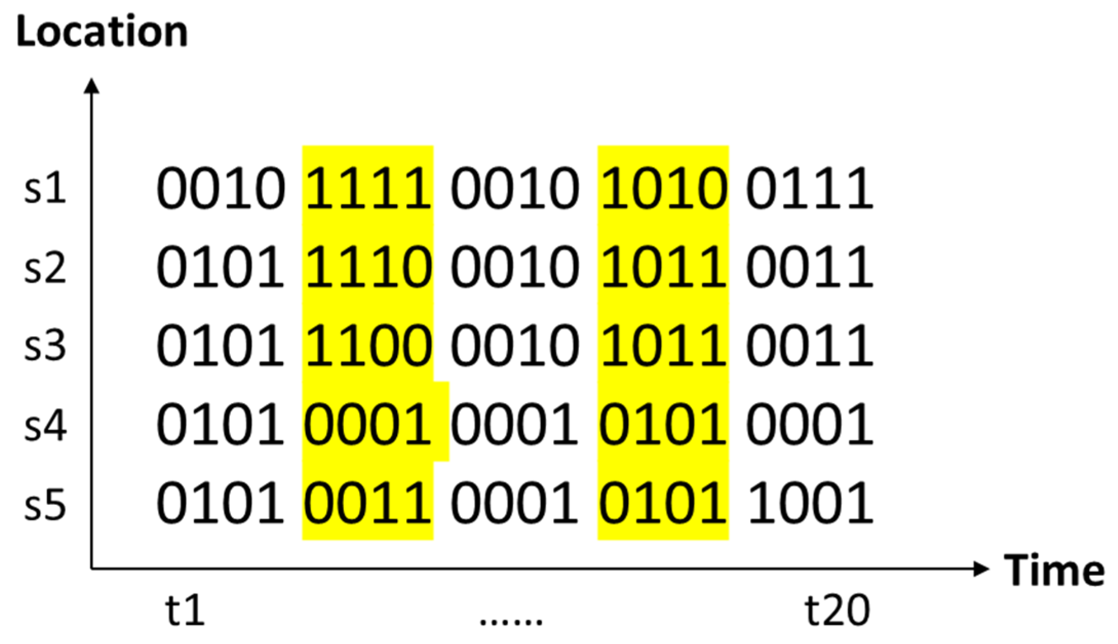
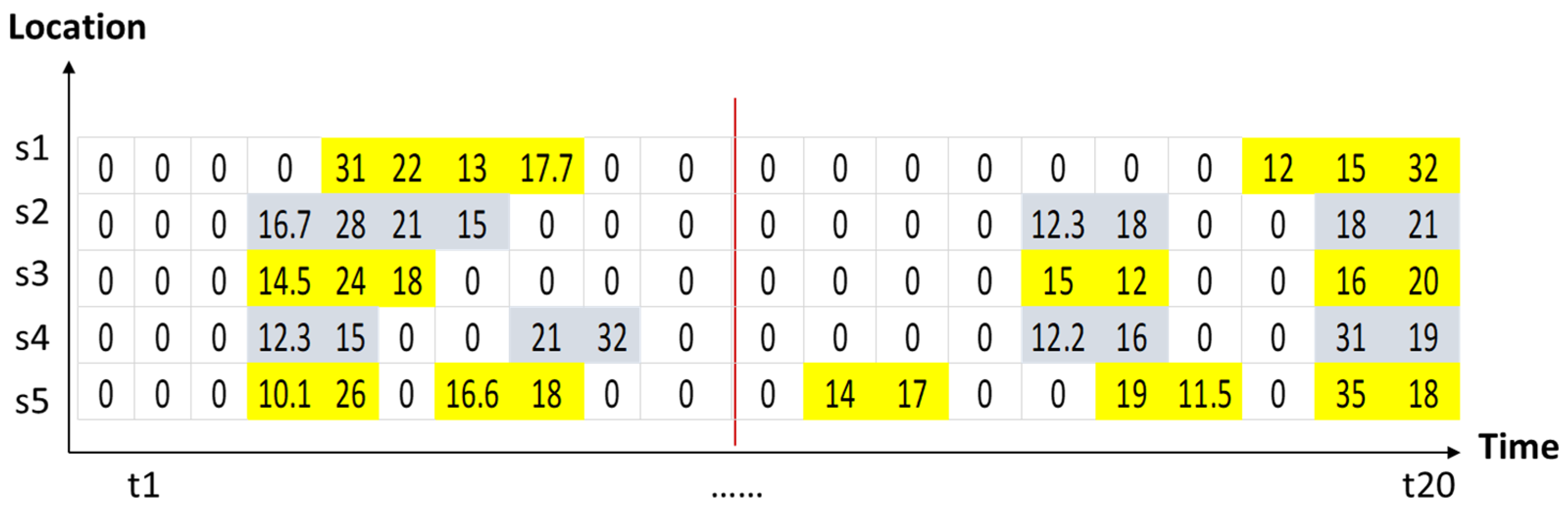
2.2. Matrix Representation of STES

For a regularly sampled time series, the set of timestamps T forms a discrete set, with observations spaced at uniform time intervals. Given s locations and t timestamps, a space-time series dataset can be represented with a s × t matrix where locations correspond to rows and timestamps to columns and ν represents an observed variable.
G 0 - Timestamps 1 , 2 , 3 , , t Spatial   locations   1 , 2 , 3 , , s v 11 , v 12 , v 13 , , v 1 t v 21 , v 22 , v 23 , , v 2 t v 31 , v 32 , v 33 , , v 3 t v s 1 , v s 2 , v s 3 , , v s t
G0-Timestamps represent the finest temporal granularity as described by Shahar [30], here corresponding to the time series sampling rate. Each value potentially corresponds to a status change, which could define a timestamped event or the start or end of an interval event. As noted above, events are identified based on different user defined functions such as threshold based, pattern-based, or learning based [31]. For simplicity, in the following definitions, we assume use of a threshold, but the approach is generalizable to other event detection approaches [32]. A temporal granularity in integer unit Gi scaled from G0 (e.g., hour to day, day to week) is specified by a user based on application domain considerations. At each observation location s, an event sequence is formed at the Gi scale after eventization. The event sequences for all locations form an initial STES matrix. In the eventization process, the dimension can be further reduced through removing rows and columns without events in locations across all Gi-timestamps or Gi-timestamps across all locations. Following this data reduction, we may have n locations and Gi granularity of m timestamps, in which the STES are represented as n × m matrix ( n s   and   m t ).
G i   Timestamps   1 ,   2 ,   3 ,   , m Spatial   locations   1 ,   2 ,   3 ,   , n e 11 , e 12 , e 13 , , e 1 m e 21 , e 22 , e 23 , , e 2 m e 31 , e 32 , e 33 , , e 3 m e n 1 , e n 2 , e n 3 , , e n m
We identify four different cases corresponding to timestamped versus interval events and qualitative versus quantitative. For the case of nominal values, appearance of a user specified nominal category or label at a timestamp indicates the occurrence of an event. For this case the event value is defined as follows:
e i j = n a         i f   v i j = m i s s i n g   d a t a 1             i f   v i j t h r e s h o l d ,   o r                 i f   v i j = d e f i n e d   n o m i n a l   v a l u e 0             o t h e r w i s e i = 1 ,   2 ,   3 ,   , n ; j = 1 , 2 , 3 , , m
where all timestamped observations ( v i j ) are ordinal, interval or ratio values, the corresponding event value eij may retain the original observation value or be subjected to some data transformation such as logarithm, percentage or normalization. Given a threshold for defining an event instance, sequences in this case can be represented as follows:
e i j = n a         i f   v i j = m i s s i n g   d a t a 0         i f   v i j < t h r e s h o l d v i j   o r   v i j         i f   v i j t h r e s h o l d v i j   i s   t r a n s f o r m e d   v i j i = 1 ,   2 ,   3 ,   , n ; j = 1 , 2 , 3 , , m
An interval event occurs when the defining event conditions persist for more than one G1 timestamp. As long as we determine the smallest temporal granularity in a specific study or system, we can represent an interval event sequence through the same timestamped event matrix as described above. The case for interval events with categorical values can be defined according to Equation (5):
e i j ,   e i j + 1 ,   ,   e i j + Δ t = n a       i f   v i j ,   v i j + 1 ,   ,   v i j + Δ t = m i s s i n g   d a t a 1       i f   v i j ,   v i j + 1 ,   ,   v i j + Δ t t h r e s h o l d o r ,     i f   v i j ,   v i j + 1 ,   ,   v i j + Δ t = d e f i n e d   n o m i a l   s c a l e Δ t 1 0       o t h e r w i s e i = 1 ,   2 ,   3 ,   , n ; j = 1 , 2 , 3 , , m
The case for interval events with ordinal or interval/ratio values can be defined according to Equation (6):
e i j ,   e i j + 1 ,   ,   e i j + Δ t = n a         i f   v i j ,   v i j + 1 ,   ,   v i j + Δ t = m i s s i n g   d a t a 0         i f   v i j ,   v i j + 1 ,   ,   v i j + Δ t < t h r e s h o l d v i j ,   v i j + 1 ,   ,   v i j + Δ t   o r   v i j ,   v i j + 1 ,   , v i j + Δ t                   i f   v i j ,   v i j + 1 ,   ,   v i j + Δ t   t h r e s h o l d                 v i j ,   v i j + 1 ,   , v i j + Δ t : t r a n s f o r m e d   v i j ,   v i j + 1 ,   ,   v i j + Δ t                   Δ t 1 0   o t h e r w i s e i = 1 ,   2 ,   3 ,   , n ; j = 1 , 2 , 3 , , m
For all interval events with no internal variation within the interval, i.e., with a constant event class level, the defined interval events are as described in Equation (6):
e i j = e i j + 1 = = e i j + Δ t f r o m   v i j = v i j + 1 = = v i j + Δ t   o r   v i j = v i j + 1 = = v i j + Δ t

2.3. Development of Similarity Measures for Spatiotemporal Event Sequences

The matrix framework presented above provides a flexible method to investigate sequence similarity over space for the same time windows. In this context, we consider the event sequence similarity as the level of co-occurring timestamped events for a certain time period for two or more locations. We can vary the selection of a time window based on the sampling frequency of the observation data and a target event granularity (e.g., drought events which may be defined as over 10 days of no rain need a larger time window relative to heavy precipitation events). We present similarity measures for five situations: (a) binary timestamped events (no consideration of variable class levels or magnitude), (b) timestamped events with variable class levels or magnitude, (c) interval events considering time overlaps only, (d) interval events with constant nominal or ordinal labels and time overlaps, and (e) interval events with a range of real values and time overlaps.
We follow the concept of Jaccard similarity [33] but consider the order of individual event elements within each event sequence. The intersection between two sets of spatiotemporal event sequences means the common events must “co-occur” in both sequences, and the union refers to all events in either sequence. The measure of co-occurrence is demonstrated by the following example:Ijgi 10 00594 i001
Given the two spatiotemporal timestamped event sequences with 10 timestamps, we compute the similarity between the two spatiotemporal event sequences as:
s i m e s 1 ,   e s 2 = e s 1 e s 2 e s 1 e s 2 = 5 10 = 0.5
where, e s 1 , e s 2 are two spatiotemporal event sequences from two locations S1, S2; t1, t2, …, t10 are 10 timestamps. The intersection between two event sequences is the number of co-occurring events between them. We discuss this similarity measure in more detail for five different situations in the following sections.

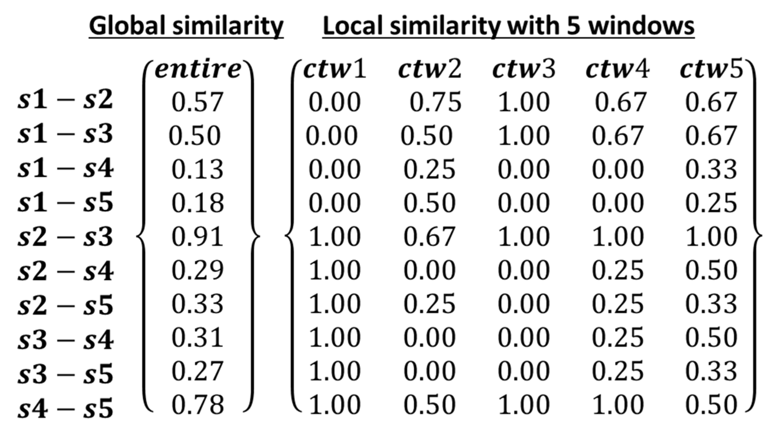
2.3.1. Similarity Measures between Event Sequences without Considering Event Magnitude

First, we compute the level of pairwise co-occurrence between two event sequences e s 1 and e s 2 , c o _ o c c u r e s 1 ,   e s 2 , by simply counting the number of punctual events with the same occurrence time appearing in both e s 1 and e s 2 . So, the global (long duration) similarity between event sequences can be calculated as below:
s i m g l o b l a l e s 1 ,   e s 2 = c o _ o c c u r e s 1 ,   e s 2 e s 1 e s 2
where s i m g l o b l a l e s 1 ,   e s 2 —global similarity between event sequences e s 1   and   e s 2 , meaning overall similarity between two event sequences over a long user specified duration, c o _ o c c u r e s 1 ,   e s 2 —co-occurring number of events between sequences e s 1   and   e s 2 , e s 1 e s 2 —cardinality of the union of two event sequences e s 1   and   e s 2 .
In contrast to global similarity, we introduce a user defined local comparison temporal window (ctw) (equivalent to a moving window), for which local (short duration) similarity is calculated as:
s i m l o c a l e s 1 _ c t w i ,     e s 2 _ c t w i = c o _ o c c u r e s 1 _ c t w i ,     e s 2 _ c t w i e s 1 _ c t w i e s 2 _ c t w i
where, i = 1 ,   2 ,   3 ,   ,   k ; k = T e m p o r a l   L e n g t h   o f   E v e n t   S e q u e n c e c t w , the number of time window chunks in an event sequence; e s 1 _ c t w i e s 2 _ c t w i , cardinality of the union of two corresponding subsequences of two event sequences in the same c t w . For each pair of spatiotemporal event sequences, we have k local similarities in an ordered list, represented as s i m l o c a l 1 ,     s i m l o c a l 2 ,     s i m l o c a l 3 ,   ,   s i m l o c a l   k .

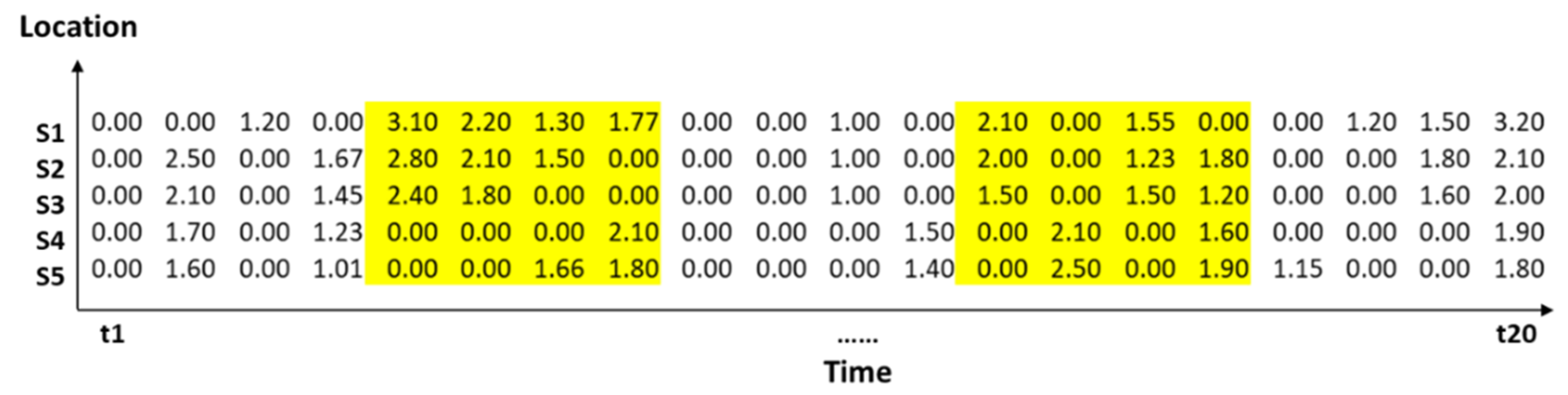
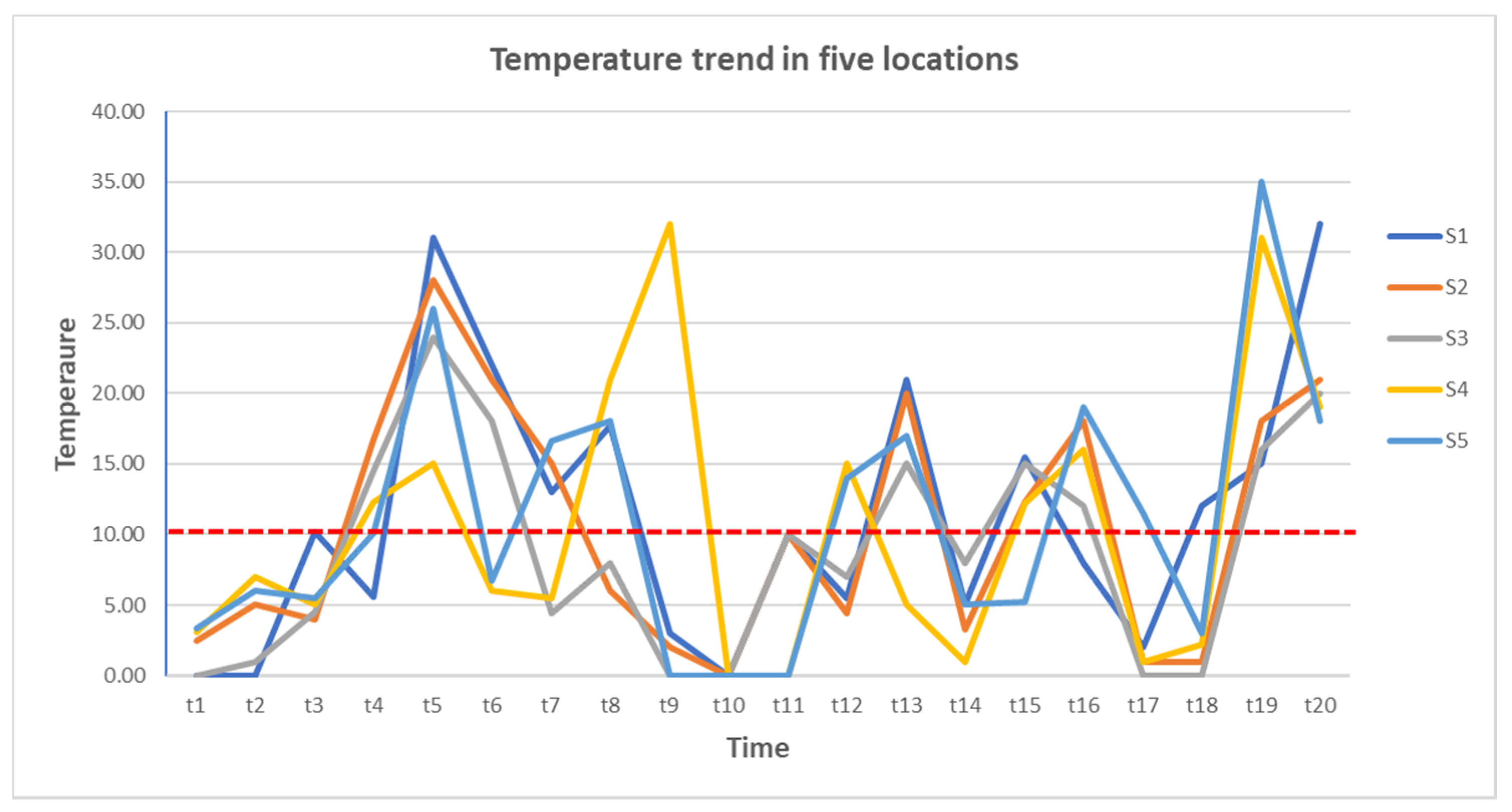
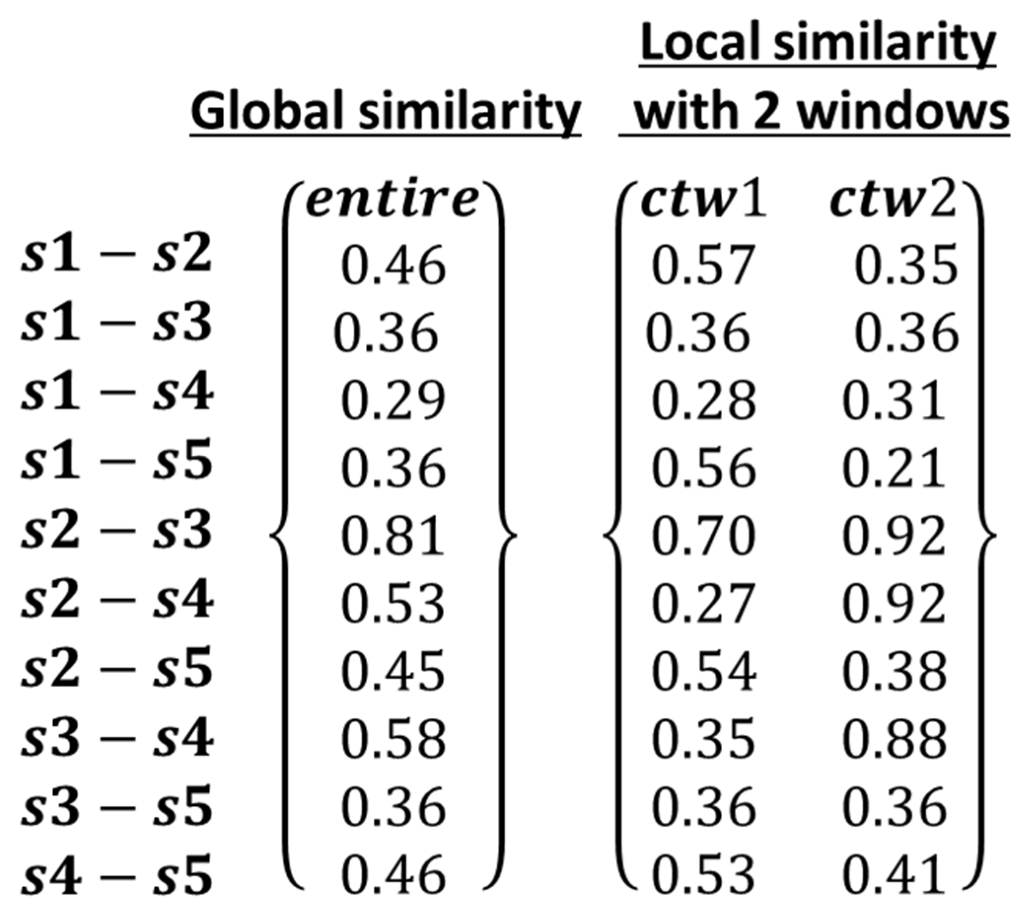
2.3.2. Similarity Measures between Event Sequences Considering Event Magnitude

We first find all co-occurrence time points between two event sequences e s 1 and e s 2 , and then we calculate the similarity between two individual events at the co-occurrence timestamp based on their level of measurement. We have two similarity calculation situations. First, if event values are interval or ratio level, the global similarity can be calculated as below:
s i m g l o b l a l e s 1 ,   e s 2 = j = 1 C 1 A b s l e v e s 1 j l e v e s 2 j e s 1   e s 2
Second, if event levels are ordinal attribute based, the formula becomes:
s i m g l o b l a l e s 1 ,   e s 2 = j = 1 C 1 A b s l e v e s 1 j l e v e s 2 j n 1 e s 1   e s 2
where,
  • s i m g l o b l a l e s 1 ,   e s 2 —global similarity between event sequences e s 1   and   e s 2 ,
  • e s 1 j ,   e s 2 j   —the event levels of two corresponding co-occurring events in e s 1 and e s 2 at timestamp j , inherited from original measurements,
  • l e v e s 1 j , l e v e s 2 j —the relative event levels of two corresponding co-occurring events in e s 1 and e s 2 at timestamp j , respectively:
l e v e s 1 j = e s 1 j e s 1 j + e s 2 j   and   l e v e s 2 j = e s 2 j e s 1 j + e s 2 j
where,
  • C —the total number of co-occurring timestamps,
  • A b s l e v e s 1 j l e v e s 2 j —absolute value of difference between relative event levels of two corresponding co-occurring events in e s 1 and e s 2 at time stamp j ,
  • e s 1 e s 2 —cardinality of the union of two event sequences e s 1   and   e s 2 ,
  • n—the number of ordinal attribute-based event levels.
Similarly, we can characterize the local similarity between event sequences by the following Equation (11) for interval/ratio attribute-based events and (12) for ordinal attribute-based events:
s i m l o c a l e s 1 _ c t w i ,     e s 2 _ c t w i = j = 1 c 1 A b s l e v   e s 1 c t w i j l e v   e s 2 c t w i j   e s 1 c t w i     e s 2 c t w i
and
s i m l o c a l e s 1 _ c t w i ,   e s 2 _ c t w i = j = 1 C 1 A b s ( l e v   e s 1 c t w i j l e v e s 2 c t w i j n 1 e s 1 c t w i j     e s 2 c t w i j
where, i = 1 ,   2 ,   3 ,   ,   k ;   k = T e m p o r a l   L e n g t h   o f   E v e n t   S e q u e n c e c t w ,   c is the number of co-occurring time points in c t w , e s 1 c t w i j   e s 2 c t w i j , cardinality of the union of two corresponding subsequences of two event sequences in the same c t w . As before for each pair of spatiotemporal event sequences, we have k local similarities in an ordered list, represented as s i m l o c a l 1 ,   s i m l o c a l 2 ,   s i m l o c a l 3 ,   ,   s i m l o c a l k .
We note that the approaches for measuring sequence similarity as described above apply also to interval event sequences. We simply transform interval event sequences to punctual event vectors to form a matrix.

3. Results and Discussion

3.1. Implementation Examples

In this section we use simulated precipitation and temperature datasets to demonstrate the transformation of raw space- time series observations to event sequence matrices based on the event definitions described in the previous section. We calculate global and local pairwise event sequence similarities according to the steps described above. The transformation to STES matrices and the similarity measure calculations have been developed as R functions (see the link for software availability). The first two experiments cover timestamped events based on simulated precipitation measurements for 5 locations and 20 timestamps as shown in Table 1. We note that these timestamps could apply to different temporal granularities, but some minimum granularity is considered a punctual timestamp.
Situation 1.
We define precipitation 1 inch as events from the dataset in Table 1 and based on Equation (3) we transform the measurements to a matrix of binary punctual events:
Temporal   points ( 1 ,   2 ,   3 ,   ,   20 ) Spatial   locations ( 1 ,   2 ,   3 ,   4 ,   5 ) 0 0 1 0 1 1 1 1 0 0 1 0 1 0 1 0 0 1 1 1 0 1 0 1 1 1 1 0 0 0 1 0 1 0 1 1 0 0 1 1 0 1 0 1 1 1 0 0 0 0 1 0 1 0 1 1 0 0 1 1 0 1 0 1 0 0 0 1 0 0 0 1 0 1 0 1 0 0 0 1 0 1 0 1 0 0 1 1 0 0 0 1 0 1 0 1 1 0 0 1
In an alternate view of this matrix seen in Figure 4. we show local comparative temporal windows based on 4 timestamps, i.e., c t w = 4 :
The pairwise global similarity and local similarity between event sequences were calculated based on Equations (7) and (8). Here, c t w = 4 , so we have 5 chunks of subsequences for each original event sequence. The pairwise similarity measures between event sequences of 5 locations is shown in Figure 5.
By intuition, the event sequences in locations s2 and s3 are more similar than other pairs with only one mismatch, which is reflected in the global similarity matrix with the highest score of 0.91. The lowest similarity score is between s1 and s4 event sequences with only two co-occurring events. The rest of the similarity scores for other pairwise comparisons reflect their closeness in terms of co-occurrences.
Situation 2.
We again extract precipitation 1 inch-events from the dataset in Table 1 but now consider the magnitude of the precipitation 1 inch by retaining the original observation values. Based on the transformation rules described in Equation (4) we obtain the event matrix with event levels as follows:
Temporal   points ( 1 ,   2 ,   3 ,   ,   20 ) Spatial   locations ( 1 ,   2 ,   3 ,   4 ,   5 ) 0 0 1.2 0 3.1 2.2 1.3 1.77 0 0 1 0 2.1 0 1.55 0 0 1.2 1.5 3.2 0 2.5 0 1.67 2.8 2.1 1.5 0 0 0 1 0 2 0 1.23 1.8 0 0 1.8 2.1 0 2.1 0 1.45 2.4 1.8 0 0 0 0 1 0 1.5 0 1.5 1.2 0 0 1.6 2 0 1.7 0 1.23 0 0 0 2.1 0 0 0 1.5 0 2.1 0 1.6 0 0 0 1.9 0 1.6 0 1.01 0 0 1.66 1.8 0 0 0 1.4 0 2.5 0 1.9 1.15 0 0 1.8
The alternate view of this event matrix is shown in Figure 6. Where Equations (9) and (11) are used to calculate the global and local similarity respectively:
From the similarity matrix in Figure 7 we can see the change of similarity scores from the results shown in Figure 5 that do not take event magnitude into consideration. While all scores in Figure 7 decrease compared to Figure 5, the overall rankings of these scores are the same. This indicates that refinement of event levels and additional attributes of events incorporated into the similarity measure can affect the similarity values but rankings between event sequences remain stable.
The following examples for interval events are based on the temperature graph for five locations shown in Figure 8.
Situation 3.
Here we identify interval events ≥ 10 °C from high frequency temperature measurements at 5 locations. Assume that a minimum temporal granularity is specified (e.g., day, hour) such that we can obtain the measurements at all time points (t1, t2, …, t20) as in the dataset shown in Table 2. Using Equation (5), we obtain interval events as a sequence of contiguous 1s in a binary event matrix.
The sequence of contiguous 1’s represents interval events, but these are processed as punctual events in the event sequence matrix:
Temporal   points ( 1 ,   2 ,   3 ,   ,   20 ) Spatial   locations ( 1 ,   2 ,   3 ,   4 ,   5 ) 0 0 0 0 1 1 1 1 0 0 0 0 0 0 0 0 0 1 1 1 0 0 0 1 1 1 1 0 0 0 0 0 0 0 1 1 0 0 1 1 0 0 0 1 1 1 0 0 0 0 0 0 0 0 1 1 0 0 1 1 0 0 0 1 1 0 0 1 1 0 0 0 0 0 1 1 0 0 1 1 0 0 0 1 1 0 1 1 0 0 0 1 1 0 0 1 1 0 1 1  
The alternative view of the interval event matrix in the example of Situation 3 can be seen in Figure 9. In this figure, we also assume that the comparative temporal window has 10 timestamps, i.e., ctw = 10 such that we have only 2 subsequences.
The pairwise global similarity and local similarity between event sequences is calculated with the Formulas (7) and (8). Here, c t w = 10 , so we have 2 chunks of subsequences for each original event sequence. The pairwise similarity matrices between event sequences for the 5 locations is shown in Figure 10.
The event sequences for locations s2 and s3 in Figure 10 are more similar than other pairs with only one mismatch at one timepoint, which is reflected in the global similarity matrix with the highest score of 0.88. The lowest similarity is between s1 and s4 event sequences with only four co-occurring timepoints and a relatively long union of events. The rest of the similarity scores reasonably reflect their actual closeness.
Situation 4.
For the interval events of Situation 3 with the consideration of event level, i.e., the variation of event values within the interval, we obtain a matrix of interval events based on Equation (7) as below:
The sequence of contiguous values represents interval events, but these are processed as punctual events in the event sequence matrix:
Temporal   points ( 1 ,   2 ,   3 ,   ,   20 ) Spatial   locations ( 1 ,   2 ,   3 ,   4 ,   5 )   0 0 0 0 31 22 13 17.7 0 0 0 0 0 0 0 0 0 12 15 32 0 0 0 16.7 28 21 15 0 0 0 0 0 0 0 12.3 18 0 0 18 21 0 0 0 14.5 24 18 0 0 0 0 0 0 0 0 15 12 0 0 16 20 0 0 0 12.3 15 0 0 21 32 0 0 0 0 0 12.2 16 0 0 31 19 0 0 0 10.1 26 0 16.6 18 0 0 0 14 17 0 0 19 11.5 0 35 18
The alternative view of the interval event matrix in the example of Situation 4 is represented in Figure 11. In this figure, we assume that the comparative temporal window has 10 timestamps, i.e., ctw = 10.
The pairwise global similarity and local similarity between event sequences is calculated with Equations (9) and (11) for this situation. Here, c t w = 10 , so we have 2 chunks of subsequences for each original event sequence. The pairwise similarity matrices between event sequences of 5 locations is shown in Figure 12.
This situation considers the internal variation within an interval event along with co-occurrences. We can compare the similarity scores in Figure 12 with those in Figure 10. Like Situation 2, the overall similarity values decrease compared to the situations without considering event magnitude. We can see here the event sequences at locations s2 and s3 in Figure 12 are still more similar than other pairs with slight variations of event values between co-occurring timepoints, which can be reflected in the global similarity matrix with the highest score of 0.81. The lowest similarity (0.29) remains between s1 and s4 as in Situation 3. The rest of the similarity scores for other pairwise comparisons also reasonably reflect an intuitive sequence closeness.
A Special Case in Situation 4.
If the temperature measurements are recorded as an average value for every four days as shown in Table 3.
We can transform this dataset to a matrix of interval events with event levels based on Equation (6) as shown in the matrix below:
Temporal   points ( 1 ,   2 ,   3 ,   ,   20 ) Spatial   locations ( 1 ,   2 ,   3 ,   4 ,   5 ) 0 0 0 0 22 22 22 22 12 12 12 12 0 0 0 0 31 31 31 31 0 0 0 0 28 28 28 28 14 14 14 14 0 0 0 0 26 26 26 26 11 11 11 11 24 24 24 24 11 11 11 11 0 0 0 0 28 28 28 28 14 14 14 14 25 25 25 25 18 18 18 18 0 0 0 0 33 33 33 33 0 0 0 0 18 18 18 18 12 12 12 12 15 15 15 15 24 24 24 24
The alternative view of the interval event matrix for this example of average temperature can be seen in Figure 13. In this figure, we also assume that the comparative temporal window has 10 timestamps, i.e., ctw = 10.
The pairwise global similarity and local similarity between event sequences can be calculated with Equations (9) and (11). Here, ctw = 10, so we have 2 chunks of subsequences for each original event sequence. The pairwise similarity matrices between event sequences of 5 locations is shown in Figure 14.
Intuitively we can see the event sequences between locations s1 and s2, and between locations s3 and s4 in Figure 14 are more similar than other pairs with all co-occurring events of similar value at most timepoints, which can be reflected in the global similarity matrix with the highest score of 0.91 and 0.90. The lowest similarity is 0.51 between s4 and s5 event sequences with three co-occurring events of different significance and two mismatched events.

3.2. Performance Evaluation

In this section we present our experimental evaluation of the accuracy and speed of different similarity measures with some synthetic datasets. In the first experiment, we compared the speed for computing similarity matrices using the small dataset used in this section. For the second, we used K-nearest neighbor (k-NN) classification with different similarity measures for comparing classification accuracy and efficiency.

3.2.1. Execution Speed for a Binary Event Matrix

The purpose of this experiment is to assess processing times for the timestamp locked Jaccard based similarity described in this paper (STES.sim1, see the software availability link). We compared STES.sim1 with generic edit distance in R (EditD Dynamic), and two functions of Edit Distance and original Jaccard similarity from the R package Rstringdist. The dataset contains 20 timestamps and 5 locations so we can generate a 5 × 5 similarity matrix. Microbenchmarks [34] in R was used to record the time elapsed for each similarity algorithm in the same similarity matrix generation function in R. The result indicated that STES.sim1 outperformed edit distance by a factor of 10 (Table 4).

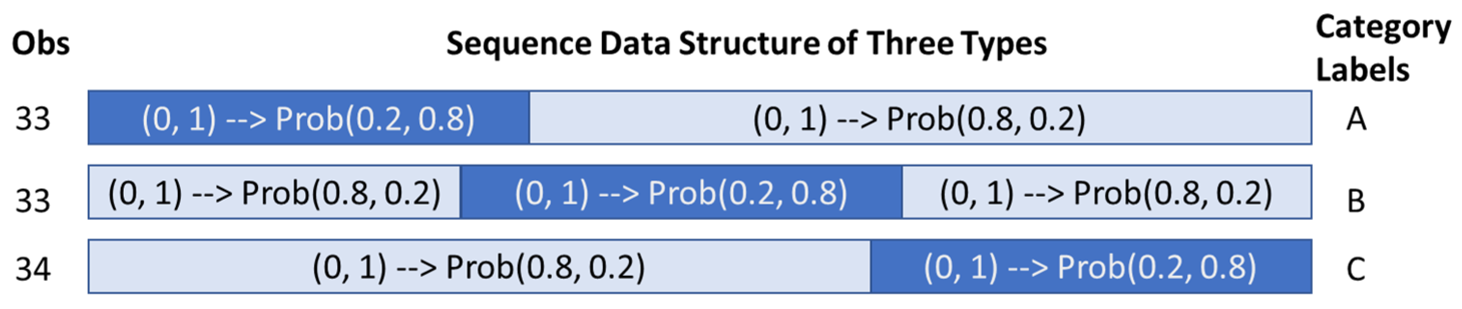
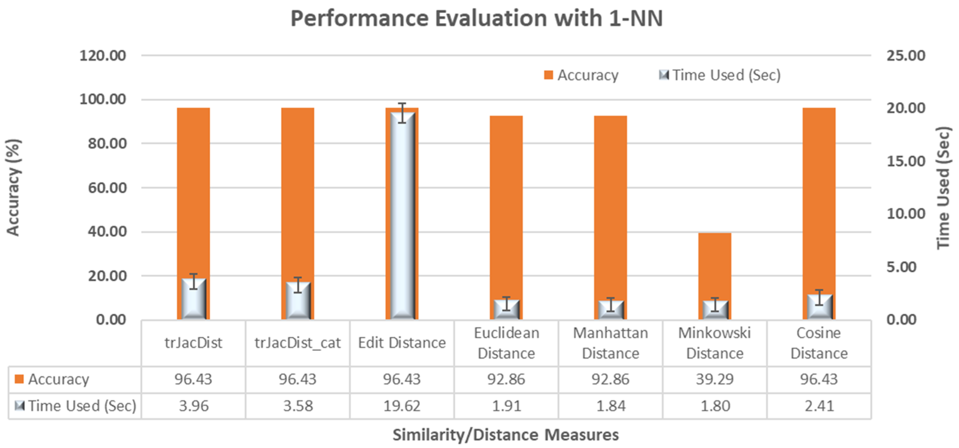
3.2.2. Accuracy Evaluation with Synthetic Datasets Using 1-NN Classifier

K-NN is a conventional non-parametric classifier, used widely as the baseline classifier for solving many classification problems [35,36]. It is based on measuring the distances or similarities between a test data set and each of the training data to decide the final classification output. When proposing a new distance or similarity measure, 1-NN accuracy was strongly recommended for testing [37]. Note that this does not exclude the additional other trainings and tests with different K values. Here, however, the 1-NN test has the advantage of having no parameters and allowing comparisons between similarity measures.
Synthetic dataset 1: This dataset contains 100 event sequences (records) with 50 timestamped fields of binary values (0, 1) representing whether the event occurred or not. The test uses 3 different event distribution patterns (groups or classes) labeled by A, B and C. The sample function in R with the prob argument was used to control density and order of event occurrences. The first pattern (Label A) is characterized with the first 20 timestamps having a higher probability (0.8) of event occurrence and the remainder with lower probability (0.2). In the second pattern (Label B) the subsequence of higher probability of event occurrence is placed in the middle, and in the third pattern (Label C), the higher probability occurrence region is placed at the end. The event data structure of these three patterns and the observation number of each pattern are graphically depicted in Figure 15.
We should note that the binary data (0, 1) can represent either two categories or actual values of 0 and 1. Therefore, both category-based and value-based similarity measures can be applied to this dataset. In this evaluation experiment, the category-based measures include Edit Distance and time-restricted Jaccard Distance for category data (trJacDist-cat) developed in this paper, and the value-based distance measures are Euclidean, Manhattan, Minkowski, and Cosine Distance. When running 1-NN classification test, the dataset with three patterns is first randomized and then divided into 70% training and 30% test set for the experimental setup. Hence, there are 70 training event sequences and 30 test sequences on which classification was performed. The effectiveness of a similarity measure in this experiment is evaluated with accuracy for classifying three patterns of event sequences (Label A, B, and C) and time for completing the task. To capture the fluctuation of time used for each task due to internal computer operation system, we run each 1-NN test for each similarity measure 15 times to compute the error bars.
Using seven similarity measures carried out with 1-NN classification for the dataset mentioned above, Figure 16 shows the comparison of accuracy and time elapsed to complete the given task. The effectiveness of different similarity measures can be seen by comparing the accuracy and time required to complete the task. While the same accuracy can be achieved with trJacDist/trJacDist-cat and Edit Distance for classifying this small dataset, the time required with trJacDist measure is about 5 times less than Edit Distance measure. Euclidean, Manhattan and Minkowski Distance algorithms show a time advantage over trJacDist/trJacDist-cat, but slightly lower accuracy. We note that Cosine Distance has similar accuracy but a slightly better time performance.
Synthetic dataset 2: This dataset contains 100 records (event sequences) with 128 timestamped fields of real values. As shown in Figure 17, there are three types of patterns in this dataset: sine, box, and ramp-cliff, each function of which has high level of white noise as the background noise. We excluded the Edit distance in this test as it is inappropriate for real valued data. We compared trJacDist with Euclidean, Manhattan, Minkowski, and Cosine distance-based similarity measures for evaluating the efficiency and accuracy of classification with 1-NN classifier. The dataset was also randomized and then split into 70% training and 30% test sub-datasets when running 1-NN classification. From the results shown in Figure 18 we can see that while trJacDist shows a time disadvantage against these methods it shares the same accuracy with Euclidean, Manhattan, and Cosine distance.

3.3. Application Example

We examined the feasibility of the proposed framework in the real-world application of monitoring precipitation events obtained from observation stations distributed along the Maine coast. Here we demonstrate the specific steps of eventization and similarity measures developed in this study and we address the question: Do STES that are closer in space show higher similarity measures?
The Maine Department of Marine Resources (DMR) manages the shellfish growing areas in coastal Maine based on the fecal pollution situations observed from more than 2000 monitoring stations. Precipitation events can trigger high levels of fecal coliform in shore waters and are thus of concern. Grouping of similar stations in terms of heavy rain or high precipitation events is useful for allocating the limited labor pool for long term water sampling. We used the similarity measures developed in this study to conduct clustering analysis with the high precipitation event sequences (≥1 in daily) of selected monitoring stations for 5 years.
Considering the daily precipitation is very close between nearby monitoring stations we selected 43 monitoring stations for this experiment in the shellfish growing areas that are well distributed along the Maine coast (Figure 19). With daily precipitation data of 5 years, we have an initial 43 × 1826 matrix of precipitation raw data (Table S1).
The dimensions of the raw data matrix is reduced through the eventization steps developed in this research. In this specific example, we extracted event sequences of either ≥1″ or ≥2″ precipitation for each monitoring station. Based on Equation (3) we computed the data in Table S1 with R script (STS.eventize1.R) and created the event sequence matrix of 43 × 192 (≥1″ precipitation) (Table S2) or 43 × 52 (≥2″ precipitation) (Table S3). Taking ≥1″ precipitation event sequences as an example (Table S2) and using the STES similarity measure (STES.sim1.R) from this paper, we created the similarity matrix of 43 × 43 (Table S4) between selected test monitoring stations. We transformed these similarity data into distance data to conduct hierarchical clustering analysis [38] using the hclust R function with linkage method Ward.D2.
Figure 20 shows the clustering results from using STES similarity on event sequences of ≥1 in precipitation during 5 years in 43 locations (monitoring stations) as a heatmap and distance-based cluster dendrogram.
The results show the emergence of five clusters (groupings of event sequences that are most similar). The heatmap and cluster dendrogram indicate that these clusters are in fact spatial clusters indicating that for this case, sequences that are close in space tend to be more similar. These results can provide decision makers with more information for arranging the labor within each region (cluster) along the Maine coast to collect water samples for fecal coliform measurements from selected stations.

4. Conclusions

In this paper, we have demonstrated a matrix-based representation of spatiotemporal event sequences for unifying punctual and interval events. These similarity measures along with the univariate spatiotemporal event matrices for event data storage discussed above provide a novel method and an alternative foundation for further event sequence pattern discovery. A comparison of event sequence similarity is important for detecting co-occurrence patterns and investigating the influence of event sequences of interest. We assume that similar event sequences indicate a similar process structure and potential shared causal mechanisms.
Based on the analysis of sequence properties for four situations and one special case that consider event co-occurrences and event levels, we have proposed corresponding similarity measures for pairwise comparisons for punctual and interval events and for whole or long duration sequences or their subsequences. The experimental results with simulated datasets showed that these similarity scores between spatiotemporal event sequences reasonably represent perceived closeness.
A comparative evaluation against other similarity algorithms shows the same or better accuracy results. Our method shows a time disadvantage against the real valued methods but a substantial time advantage over the qualitative Edit Distance. Overall, our approach has the advantages of flexibility in that it can accommodate both qualitative and quantitative event values as well as both punctual and interval events.
We recognize some limitations in the current research. This research establishes a framework of matrix representations and similarity development for univariate event sequences of different types. It does not yet handle similarity assessment for multivariate event sequences. Such an extension requires some modification of the matrix representation and similarity measures which will be addressed in future work. In the current work we demonstrate fixed matrix sizes which can be chunked into smaller subsequence sets for local versus global similarity computations. For future work, an extension that addresses streaming events from monitoring stations would be a useful addition. The addition of temporal logic operations and extensions to consider lagged sequence alignment similarity rather than the time locked case are other considerations for future work. Furthermore, we have not tested the current methods on big data. Future work will focus on the evaluation extensive real datasets from environmental monitoring or other domains. Currently our STES representation includes the intervals between event occurrences. For sequences in which event occurrences may be sparse with long intervening intervals we are considering approaches for sparse matrices. Lastly, we also consider extensions to detect complex events of interest, and incorporation of our methods into Complex Event Processing (CEP) systems.

Supplementary Materials

The following are available online at https://www.mdpi.com/article/10.3390/ijgi10090594/s1, Table S1: Precipitation data of 43 monitoring stations in the Maine coast (2010–2014). Table S2: Event sequence matrix of 43 × 192 from eventization based on ≥1″ precipitation. Table S3: Event sequence matrix of 43 × 52 from eventization based on ≥2″ precipitation. Table S4: Similarity matrix of 43 × 43 from the event sequence matrix of Table S2.

Author Contributions

Conceptualization, Fuyu Xu and Kate Beard; methodology, Fuyu Xu and Kate Beard; software, Fuyu Xu and Kate Beard; validation, Fuyu Xu and Kate Beard; investigation, Fuyu Xu and Kate Beard; writing—original draft preparation, Fuyu Xu; writing—review & editing, Kate Beard; supervision, Kate Beard. All authors have read and agreed to the published version of the manuscript.

Funding

This research received no external funding.

Institutional Review Board Statement

Not applicable.

Informed Consent Statement

Not applicable.

Data Availability Statement

The data presented in this study are available the supplementary material here.

Conflicts of Interest

The authors declare no conflict of interest.

Software Availability

Name: (1) STS.eventize, STS.eventize1, STS.eventize2, and STS.eventize3 (conversion of space-time series to event sequences considering either variation of events or not based on domain context and user’s requirements), and (2) STES.sim1, STES.sim2, STES.sim3, STES.simOr, and STES.simOr2 (Calculation of global and local similarities between event sequences based on sequences of different event types and generation of global and local similarity matrices as user defined local granularity or window size). Developers: Fuyu Xu and Kate Beard. Program language: R. Software requirement: R console or RStudio. Source code: https://frank888.github.io/STES_similarity.html (accessed on 8 September 2021).

References

  1. Bollobas, B.; Das, G.; Gunopulos, D.; Mannila, H. Time-series similarity problems and well-separated geometric sets. In Proceedings of the Thirteenth Annual Symposium on Computational Geometry, Nice, France, 4–6 June 1997; pp. 454–456. [Google Scholar]
  2. Fu, T.-C. A review on time series data mining. Eng. Appl. Artif. Intell. 2011, 24, 164–181. [Google Scholar] [CrossRef]
  3. Du, F.; Shneiderman, B.; Plaisant, C.; Malik, S.; Perer, A. Coping with volume and variety in temporal event sequences: Strategies for sharpening analytic focus. IEEE Trans. Vis. Comput. Graph. 2016, 23, 1636–1649. [Google Scholar] [CrossRef] [PubMed]
  4. Shurkhovetskyy, G.; Andrienko, N.; Andrienko, G.; Fuchs, G. Data abstraction for visualizing large time series. Comput. Graph. Forum 2018, 37, 125–144. [Google Scholar] [CrossRef]
  5. Yeh, C.-C.M.; Zhu, Y.; Ulanova, L.; Begum, N.; Ding, Y.; Dau, H.A.; Zimmerman, Z.; Silva, D.F.; Mueen, A.; Keogh, E. Time series joins, motifs, discords and shapelets: A unifying view that exploits the matrix profile. Data Min. Knowl. Discov. 2018, 32, 83–123. [Google Scholar] [CrossRef]
  6. Darling, A.C.; Mau, B.; Blattner, F.R.; Perna, N.T. Mauve: Multiple alignment of conserved genomic sequence with rearrangements. Genome Res. 2004, 14, 1394–1403. [Google Scholar] [CrossRef] [Green Version]
  7. Maurya, M.R.; Rengaswamy, R.; Venkatasubramanian, V. Fault diagnosis using dynamic trend analysis: A review and recent developments. Eng. Appl. Artif. Intell. 2007, 20, 133–146. [Google Scholar] [CrossRef]
  8. Tao, C.; Wongsuphasawat, K.; Clark, K.; Plaisant, C.; Shneiderman, B.; Chute, C.G. Towards event sequence representation, reasoning and visualization for EHR data. In Proceedings of the 2nd ACM SIGHIT International Health Informatics Symposium, Miami, FL, USA, 28–30 January 2012; ACM: New York, NY, USA, 2012; pp. 801–806. [Google Scholar]
  9. Stehle, S.; Peuquet, D.J. Analyzing spatio-temporal patterns and their evolution via sequence alignment. Spat. Cogn. Comput. 2015, 15, 68–85. [Google Scholar] [CrossRef]
  10. Prinzie, A.; Van den Poel, D. Modeling complex longitudinal consumer behavior with Dynamic Bayesian networks: An Acquisition Pattern Analysis application. J. Intell. Inf. Syst. 2011, 36, 283–304. [Google Scholar] [CrossRef]
  11. Yang, J.; McAuley, J.; Leskovec, J.; LePendu, P.; Shah, N. Finding progression stages in time-evolving event sequences. In Proceedings of the 23rd International Conference on World Wide Web, Seoul, Korea, 7–11 April 2014; ACM: New York, NY, USA, 2014; pp. 783–794. [Google Scholar]
  12. Hamming, R.W. Error detecting and error correcting codes. Bell Syst. Tech. J. 1950, 29, 147–160. [Google Scholar] [CrossRef]
  13. Levenshtein, V.I. Binary codes capable of correcting deletions, insertions, and reversals. Sov. Phys. Dokl. 1966, 10, 707–710. [Google Scholar]
  14. Jacobs, B.E.; Walczak, C.A. A generalized query-by-example data manipulation language based on database logic. IEEE Trans. Softw. Eng. 1983, SE-9, 40–57. [Google Scholar] [CrossRef]
  15. André-Jönsson, H.; Badal, D.Z. Using signature files for querying time-series data. In Proceedings of the European Symposium on Principles of Data Mining and Knowledge Discovery, Trondheim, Norway, 24–27 June 1997; Springer: Berlin/Heidelberg, Germany, 1997; pp. 211–220. [Google Scholar]
  16. Mannila, H.; Moen, P. Similarity between event types in sequences. In Proceedings of the International Conference on Data Warehousing and Knowledge Discovery, Florence, Italy, 30 August–1 September 1999; Springer: Berlin/Heidelberg, Germany, 1999; pp. 271–280. [Google Scholar]
  17. Mannila, H.; Ronkainen, P. Similarity of event sequences. In Proceedings of the TIME’97: 4th International Workshop on Temporal Representation and Reasoning, Dayton Beach, FL, USA, 10–11 May 1997; IEEE: New York, NY, USA, 1997; pp. 136–139. [Google Scholar]
  18. Wongsuphasawat, K.; Plaisant, C.; Taieb-Maimon, M.; Shneiderman, B. Querying event sequences by exact match or similarity search: Design and empirical evaluation. Interact. Comput. 2012, 24, 55–68. [Google Scholar] [CrossRef] [Green Version]
  19. Chung, N.C.; Miasojedow, B.; Startek, M.; Gambin, A. Jaccard/Tanimoto similarity test and estimation methods for biological presence-absence data. BMC Bioinform. 2019, 20, 644. [Google Scholar] [CrossRef] [PubMed]
  20. Vorontsov, I.E.; Kulakovskiy, I.V.; Makeev, V.J. Jaccard index based similarity measure to compare transcription factor binding site models. Algorithms Mol. Biol. 2013, 8, 1–11. [Google Scholar] [CrossRef] [Green Version]
  21. Luu, V.-T.; Forestier, G.; Weber, J.; Bourgeois, P.; Djelil, F.; Muller, P.-A. A review of alignment based similarity measures for web usage mining. Artif. Intell. Rev. 2020, 53, 1529–1551. [Google Scholar] [CrossRef]
  22. Obweger, H.; Suntinger, M.; Schiefer, J.; Raidl, G. Similarity searching in sequences of complex events. In Proceedings of the 2010 Fourth International Conference on Research Challenges in Information Science (RCIS), Nice, France, 19–21 May 2010; IEEE: New York, NY, USA, 2010; pp. 631–640. [Google Scholar]
  23. Andrienko, G.; Andrienko, N.; Mladenov, M.; Mock, M.; Poelitz, C. Extracting events from spatial time series. In Proceedings of the 2010 14th International Conference Information Visualisation, London, UK, 26–29 July 2010; pp. 48–53. [Google Scholar]
  24. Mirbagheri, S.M.; Hamilton, H.J. Similarity Matching of Temporal Event-Interval Sequences. In Proceedings of the Canadian Conference on Artificial Intelligence, Online, 13–15 May 2020; Springer: Berlin/Heidelberg, Germany, 2020; pp. 420–425. [Google Scholar]
  25. Jassby, A.D.; Powell, T.M. Detecting changes in ecological time series. Ecology 1990, 71, 2044–2052. [Google Scholar] [CrossRef]
  26. Rude, A.; Beard, K. High-Level Event Detection in Spatially Distributed Time Series; Springer: Berlin/Heidelberg, Germany, 2012; pp. 160–172. [Google Scholar]
  27. Abadi, D.; Madden, S.; Lindner, W. Sensor Network Integration with Streaming Database Systems. In Data Stream Management; Springer: Berlin/Heidelberg, Germany, 2016; pp. 409–428. [Google Scholar]
  28. Hogenboom, F.; Frasincar, F.; Kaymak, U.; De Jong, F.; Caron, E. A survey of event extraction methods from text for decision support systems. Decis. Support Syst. 2016, 85, 12–22. [Google Scholar] [CrossRef]
  29. Wang, T.-Y.; Yang, M.-H.; Wu, J.-Y. Distributed Detection of Dynamic Event Regions in Sensor Networks With a Gibbs Field Distribution and Gaussian Corrupted Measurements. IEEE Trans. Commun. 2016, 64, 3932–3945. [Google Scholar] [CrossRef]
  30. Shahar, Y. A framework for knowledge-based temporal abstraction. Artif. Intell. 1997, 90, 79–133. [Google Scholar] [CrossRef] [Green Version]
  31. Yin, J.; Hu, D.H.; Yang, Q. Spatio-Temporal Event Detection Using Dynamic Conditional Random Fields. In Proceedings of the 21st International Jont Conference on Artifical intelligence, Pasadena, CA, USA, 11–17 July 2009; pp. 1321–1327. [Google Scholar]
  32. Guralnik, V.; Srivastava, J. Event detection from time series data. In Proceedings of the Fifth ACM SIGKDD International Conference on Knowledge Discovery and Data Mining, San Diego, CA, USA, 15–18 August 1999; ACM: New York, NY, USA, 1999; pp. 33–42. [Google Scholar]
  33. Jaccard, P. Étude comparative de la distribution florale dans une portion des Alpes et des Jura. Bull. Soc. Vaud. Sci. Nat. 1901, 37, 547–579. [Google Scholar]
  34. Bershad, B.; Draves, R.P.; Forin, A. Using microbenchmarks to evaluate system performance. In Proceedings of the Third Workshop on Workstation Operating Systems, Key Biscayne, FL, USA, 23–24 April 1992; IEEE: New York, NY, USA, 1992; pp. 148–153. [Google Scholar]
  35. Peterson, M.R.; Doom, T.E.; Raymer, M.L. Ga-facilitated knn classifier optimization with varying similarity measures. In Proceedings of the 2005 IEEE Congress on Evolutionary Computation, Edinburgh, UK, 2–5 September 2005; IEEE: New York, NY, USA, 2005; pp. 2514–2521. [Google Scholar]
  36. Prasath, V.; Alfeilat, H.A.A.; Lasassmeh, O.; Hassanat, A. Distance and similarity measures effect on the performance of K-nearest neighbor classifier-a review. arXiv 2017, arXiv:1708.04321. [Google Scholar]
  37. Wang, X.; Mueen, A.; Ding, H.; Trajcevski, G.; Scheuermann, P.; Keogh, E. Experimental comparison of representation methods and distance measures for time series data. Data Min. Knowl. Discov. 2013, 26, 275–309. [Google Scholar] [CrossRef] [Green Version]
  38. Ros, F.; Guillaume, S. A hierarchical clustering algorithm and an improvement of the single linkage criterion to deal with noise. Expert Syst. Appl. 2019, 128, 96–108. [Google Scholar] [CrossRef]
Figure 1. The STES problem setting. (A) An example of fixed locations of interest or observation sites distributed along the coast. (B) An example of a spatiotemporal event sequence extracted from a space-time series of precipitation with the threshold of ≥1.0 inch/24 h. Red bars represent events.
Ijgi 10 00594 g001
Figure 2. Graphical illustration of spatiotemporal event sequences (STES). (A) An example of spatiotemporal timestamped event sequences where rows represent locations each with 20 time units. (B) An example of interval event sequences for 5 locations and 20 time units.
Ijgi 10 00594 g002
Figure 3. Graphical illustration of spatiotemporal event sequences (STES) with consideration for level of measurement and variation within a single event. STES in (AC) are extracted from space-time series with interval/ratio values, and (DF) are extracted as ordinal values from space-time series. (A,D) are punctual event sequences. (B,E) are interval event sequences with no internal variation over the interval. (C,F) are interval event sequences with bounded variation within the interval consistent with an event definition. H, M and L represent high, medium and low, respectively.
Ijgi 10 00594 g003
Figure 4. A schematic view of the punctual event matrix of Situation 1 with 5 local comparison temporal windows. Blocking 2 columns in yellow is intended to improve visual separation of the local windows.
Ijgi 10 00594 g004
Figure 5. Output matrix of local similarity with five temporal windows and global similarity between five spatiotemporal event sequences from Situation 1.
Ijgi 10 00594 g005
Figure 6. A schematic view of the punctual event matrix of Situation 2 while considering varying event levels with 5 temporal comparison windows. Blocking 2 columns in yellow is for better visual separation of 5 local windows.
Ijgi 10 00594 g006
Figure 7. Output matrix including local similarity with five temporal windows and global similarity with consideration of events with variable class levels between five spatiotemporal event sequences from Situation 2.
Ijgi 10 00594 g007
Figure 8. Simulated temperature trend in 5 locations over 20 time units. Notice that the red dashed horizontal line is the applied threshold value of 10 °C.
Ijgi 10 00594 g008
Figure 9. A schematic view of the interval event matrix of Situation 3 with binary events and with two temporal windows separated by a red vertical line. Notice that the chunks blocked with blue color in horizontal orientation represent interval events.
Ijgi 10 00594 g009
Figure 10. Output matrix of local similarity with two temporal windows and global similarity between five spatiotemporal event sequences from Situation 3.
Ijgi 10 00594 g010
Figure 11. A schematic view of the interval event matrix of Situation 4 with consideration of event level and variation between starting and ending time points with 2 temporal comparison windows. Notice that the chunks blocked with colors in the horizontal orientation represent interval events.
Ijgi 10 00594 g011
Figure 12. Output matrix of global similarity and local similarity with two temporal windows considering events with ratio level values between five spatiotemporal event sequences from Situation 4.
Ijgi 10 00594 g012
Figure 13. A schematic view of the interval event matrix of Situation 4 with consideration of event level and no variation between starting and ending time points with 2 temporal comparison windows. Notice that the chunks blocked with colors in the horizontal orientation represent interval events.
Ijgi 10 00594 g013
Figure 14. Output matrix of local similarity with two temporal windows and global similarity considering event magnitude between five spatiotemporal event sequences based on the special case of Situation 4.
Ijgi 10 00594 g014
Figure 15. Schematic event sequence data structure for synthetic dataset 1 with three different mono-categorical event (0, 1) distribution.
Ijgi 10 00594 g015
Figure 16. The bar graph for accuracy and times for 1-NN using seven different similarity measures applied on synthetic dataset 1 with three classes. Note: error bars are based on 15 times of computation for the same task.
Ijgi 10 00594 g016
Figure 17. Schematic sequence data structure of three types of events (sine, box, and ramp-cliff) with real values for synthetic dataset 2.
Ijgi 10 00594 g017
Figure 18. The bar graph for accuracy and times for 1-NN using five different similarity measures applied on synthetic dataset 2 with three classes. Note: error bars are based on 15 times of computation for the same task.
Ijgi 10 00594 g018
Figure 19. Experimental sites along the Maine coast.
Ijgi 10 00594 g019
Figure 20. STES similarity-based heat map and STES distance based hierarchical clustering between monitoring stations along ME coast in >1 in precipitation events in 5 years (2010–2014).
Ijgi 10 00594 g020
Table 1. Simulated precipitation measurements in 5 locations with 20 timestamps.
t1t2t3t4t5t6t7t8t9t10t11t12t13t14t15t16t17t18t19t20
s10.220.351.200.563.102.201.301.770.300.001.000.552.100.501.550.800.201.201.502.20
s20.252.500.401.672.802.101.500.600.200.001.000.442.000.331.231.800.100.101.802.10
s30.282.100.451.452.401.800.440.800.100.001.000.701.500.801.501.200.000.001.602.00
s40.311.700.501.230.500.600.552.100.200.000.001.500.502.100.221.600.100.220.101.90
s50.341.600.551.010.600.671.661.800.100.000.001.400.702.500.521.901.150.300.501.80
Table 2. Extracted temperature measurements at 20 time points from continuous data.
t1t2t3t4t5t6t7t8t9t10t11t12t13t14t15t16t17t18t19t20
s10010.25.631221317.730105.521515.582121532
s22.55416.7282115620104.4203.312.318111821
s3014.514.524184.48001071581512001620
s43.17512.31565.5213200155112.21612.23119
s53.465.510.1266.716.618000141755.21911.533518
Table 3. Simulated averaged temperature measurements for every 4 time units in 5 locations.
t1t2t3t4t5t6t7t8t9t10t11t12t13t14t15t16t17t18t19t20
s19.89.89.89.822222222121212128.88.88.88.831313131
s29.19.19.19.12828282814141414555526262626
s3111111112424242411111111777728282828
s4141414142525252518181818999933333333
s5888818181818121212121515151524242424
Table 4. Evaluation of different similarity measures with STES similarity matrix on example data for 100 times (unit: microseconds).
AlgorithmMinlqMeanMedianuqMaxn_eval
STES.sim15035496765876572328100
EditD Dynamic4904525059425474631912,467100
EditD_Rstringdist206422802591240826255501100
Jaccard_Rstringdist186320212651216725568504100
Publisher’s Note: MDPI stays neutral with regard to jurisdictional claims in published maps and institutional affiliations.

