MCCRNet: A Multi-Level Change Contextual Refinement Network for Remote Sensing Image Change Detection

Abstract

Change detection based on bi-temporal remote sensing images has made significant progress in recent years, aiming to identify the changed and unchanged pixels between a registered pair of images. However, most learning-based change detection methods only utilize fused high-level features from the feature encoder and thus miss the detailed representations that low-level feature pairs contain. Here we propose a multi-level change contextual refinement network (MCCRNet) to strengthen the multi-level change representations of feature pairs. To effectively capture the dependencies of feature pairs while avoiding fusing them, our atrous spatial pyramid cross attention (ASPCA) module introduces a crossed spatial attention module and a crossed channel attention module to emphasize the position importance and channel importance of each feature while simultaneously keeping the scale of input and output the same. This module can be plugged into any feature extraction layer of a Siamese change detection network. Furthermore, we propose a change contextual representations (CCR) module from the perspective of the relationship between the change pixels and the contextual representation, named change region contextual representations. The CCR module aims to correct changed pixels mistakenly predicted as unchanged by a class attention mechanism. Finally, we introduce an effective sample number adaptively weighted loss to solve the class-imbalanced problem of change detection datasets. On the whole, compared with other attention modules that only use fused features from the highest feature pairs, our method can capture the multi-level spatial, channel, and class context of change discrimination information. The experiments are performed with four public change detection datasets of various image resolutions. Compared to state-of-the-art methods, our MCCRNet achieved superior performance on all datasets (i.e., LEVIR, Season-Varying Change Detection Dataset, Google Data GZ, and DSIFN) with improvements of 0.47%, 0.11%, 2.62%, and 3.99%, respectively.

1. Introduction

Change detection aims to distinguish differences in multi-temporal remote sensing images, which plays an important role in understanding land surface change, global resource monitoring, land use change, disaster assessment, visual monitoring, and urban management—forming a significant part of remote sensing image intelligent interpretation [1]. Common change detection methods feed the registered bi-temporal images into a corresponding model and output the predicted change intensity map with the same size as the original image pair, in which each pixel is predicted to be changed or unchanged.

1.1. Change Detection

Up to now, many methods have been proposed, including traditional ways and learning-based ways.

1.1.1. Traditional Methods

Traditional ways can be divided into algebraic-based, statistical-based, and feature-classification-based [2]. Algebraic-based methods measure the change by exploiting the absolute difference or ratio of pixel values such as change vector analysis [3] (CVA), which primarily determines the changed or unchanged area by comparing the vector values between bi-temporal images; however, this method has an excessive calculation interval for high-resolution remote sensing images. Statistical-based methods use region-level statistical information to build change features, which are then optimized iteratively by statistical probability theory to get the final result. Traditional models include Gaussian mixture model (GMM) and generalized statistical region merging (GSRM) [4] are generally adopted. Feature classification-based methods utilize feature mapping (e.g., support vector machine), dimension reduction (e.g., principal component analysis), and ensemble learning (e.g., decision tree) to predict the feature classification results.

1.1.2. Learning-Based Methods

Learning-based methods rely on the rapid development of deep learning algorithms. Many image classification and recognition algorithms based on convolution neural networks (CNN) give satisfactory results for remote sensing image tasks [5]. As change detection can be regarded as a pixel-level prediction task, almost all deep neural network models comply with the encoder–decoder structure to predict the change map. Daudt et al. [6] first designed three Siamese convolutional network models based on a U-net structure. Subsequently, an enhanced version of U-Net was also applied to remote sensing image change detection [7] and achieved better results. Fang et al. [8] proposed a Siamese framework according to dual learning-based domain transfer mechanism and put forward a combined loss function for solving the class im-balanced problem. Chen and Shi [9] proposed STANet, which innovatively established the spatial–temporal relationship between multi-temporal images through a self-attention mechanism, and was applied to optical remote sensing images with a Siamese network structure. However, this method was based on metric learning, thus requiring a long training iteration time, so we improved it by proposing a classification-based method. Zhang et al. [10] pointed out that current change detection methods based on deep learning have some limitations in terms of deep feature fusion and supervision, and they improved the ability to discriminate differences by inserting a spatial attention module (SAM) and channel attention module (CAM) into various level feature layers, which greatly ignored the relationship between different feature layers. Our model thus cascaded the feature pairs refined by the cross-attention module from a high layer to a bottom layer, thereby facilitating the full utilization of multi-level difference discrimination features. Meanwhile, to fully explore the relationship between a pixel and its surrounding region, we proposed a change contextual representation (CCR) module.

Change detection methods based on deep learning are mainly divided into two categories, one based on metric learning [11,12,13,14] and another based on classification [15,16,17,18,19,20,21,22]. The former regarded the change information as the similarity of feature pairs and then pulled samples belonging to the same class in the embedding space closer while simultaneously pushing samples belonging to different classes further away. DASNet [23] used a dual attention module to enhance the generalization of the extracted bi-temporal features. Finally, a metric module was adopted to predict the result by thresholding the L2-norm distance with a change map. In addition, a weighted double margin contrastive loss was put forward on the basis of a universal contrastive function. The abovementioned are metric-based methods, which are suitable for most regular change detection datasets in most cases, especially for street view images. However, they are not applicable for high-resolution bi-temporal remote sensing images, due to the difficulty of designing a more appropriate threshold in the decision module. Recently, most change detection networks based on semantic segmentation models have performed slightly better than these methods. PGA-SiamNet [24] introduced a global co-attention mechanism to emphasize the importance of correlation between the input feature pairs, thus making up the displacement of buildings in orthoimages. Adopting an identical framework, it also enhanced the post-fused bi-temporal features extracted by shared feature extraction backbone. In the decoder, multi-level features were fused as final change discriminating information. DTCDSCN [25] divided semantic segmentation and change detection into two subnetworks to make up for the lack of a boundary in the latter task and proposed improved focal loss to solve the problem of imbalanced samples. Based on the UNet++ [26] structure, DifUnet++ [27] simultaneously fused the concatenated and absolute difference features of bi-temporal images. In particular, the researchers adopted a multiple side-outs fusion strategy to reset the loss weight of different scales. Although this network structure fully utilized the fused information of the original bi-temporal images, including absolute information on the difference between feature pairs and the sum of feature maps, the experimental results were not significant due to the lack of an effective correlation between feature pairs and the context between pixels. Our attention modules greatly improved the accuracy of the corresponding datasets.

1.2. Attention Mechanism

An attention mechanism has the ability to capture long-range dependencies, so it is widely used in natural language processing, image classification, semantic segmentation, and object detection. SENet [28] first proposed a channel attention module to adaptively correct the weight ratio between channels, which simply captures channel-level long-range dependencies. By utilizing non-local theory from a global point of view, Non-local Net [29] made the receptive field no longer limited to the fixed size of the local area. That means that the model merely requires calculating the interactions between any two locations to capture long-range dependencies directly. DANet [30] proposed a position attention module and channel attention module to learn a spatial attention map and a channel attention map. The former aggregates and updates all positions by weighting on the spatial position of one feature. The latter applies attention weights to the channel dimension. In addition, DANet proved that the sum fusion of the two attention modules can further improve feature representations, which contributes to more accurate results. Different from the above, ACFNet [31] utilizes class context information instead of spatial context information as the attention weight. Specifically, it first calculates the class center by using coarse segmentation result and a feature map. Then, it corrects the pixels based on incorrect predicted results. ACFNet first introduced a class attention mechanism.

As mentioned above, methods that are based on classification perform better than metric-based ones in most cases. Based on the encoder–decoder structure, we proposed a multi-level change contextual refinement net (MCCRNet), which extracts multi-level feature pairs by a shared VGG16 [32] backbone. The extracted feature pairs are subsequently modified and strengthened through four atrous spatial pyramid cross-attention (ASPCA) modules. The decoder was constructed in the manner of coarse-to-fine, which means that the modified feature pairs with their output from the previous upsampling layer are concatenated, and the fused feature is then forwarded to the next layer to gradually restore the original image resolution. Different from other self-attention operations used in existing methods, the ASPCA module designed by us no longer takes the fused single feature as the input but uses the original multi-level feature pairs instead. Concretely, each of the feature pairs were fed into both the atrous spatial pyramid cross spatial attention (ASPCPA) module and the atrous spatial pyramid cross-channel attention (ASPCCA) module, thus establishing an interactive relationship of sharing information between dual features and simultaneously keeping the primitive dual-branch features in a steady state. Compared to the pyramid spatial–temporal attention module proposed by [6], which partitioned the image scale in a uniform manner, our pyramid structure was in the manner of atrous spatial pyramid pooling [33] (ASPP), which proved to be more effective for semantic segmentation, image classification, and object detection. Compared to the research in [29], which only enhanced dual-branch features by dual attention modules but ignored the fusing information of multi-level features, our method solved this by gradually cascading the updated feature pairs with the upsampled feature from the previous upsampling layer. To fully make use of the multi-level feature differences discrimination contextual information, we designed a change contextual representational (CCR) module, which utilized position attention and class attention mechanisms to capture the change region representations, the pixel-change region relation, and change region contextual representations. CCR first introduced the correlation between pixels and their context into change detection algorithms. This motivation came from the fact that the pixels around the changed pixels are also most likely to change. In Figure 1, the black dots represent changed pixels, and small white dots represent unchanged pixels; the rectangle represents the changed area, and the large circle represents the unchanged area. A pixel prefers to belong to the same class as its surrounding context region, which means that the class label assigned to one pixel is the category of the region/object that the pixel belongs to. We aimed to augment the change representation of one pixel by exploiting the representation of the change region of the corresponding change class, which was realized by triple operations of self-attention in this work. By fusing the upsampled features and then forwarding them into this module, the change feature could be made more robust and discriminative. The experiments proved that the ASPCA and CCR modules effectively improved the results of the change detection. In addition, to solve the problem of imbalanced change detection samples, we used the idea of cost-sensitive learning [34,35,36] to assign an adaptive weight for changed samples and unchanged sample loss. Specifically, a mathematical formula for the effective number of samples in [37] was adopted, which preferred to assign higher weights to changed pixels’ loss. Focal loss was combined to form the final effective sample number adaptively weighted loss (EAWLoss), which confirmed the effectiveness of the pixel-level binary classification task and can be extended to a multiclass task such as semantic change detection [38,39,40].

Our contributions can be summarized as follows:

(1)

We proposed a novel end-to-end framework called a multi-level change contextual refinement net (MCCRNet) for the change detection of bi-temporal remote sensing images. Compared to other methods, MCCRNet would be capable of capturing more intensive change information between bi-temporal images.

(2)

We proposed a change contextual representation (CCR) module to take advantage of changed region context. CCR first utilized the relationship between change pixels and their context through multiple self-attention operations.

(3)

We proposed an effective sample number adaptively weighted loss for solving the sample class-imbalanced problem.

2. Materials and Methods

In this section, we describe the details of the proposed method. Firstly, we present our network multi-level change contextual refinement net (MCCRNet) in Section 2.1; then, in Section 2.2, we introduce the experimental datasets in our work and propose the effective sample number adaptively weighted loss in Section 2.3. Finally, we describe the experimental implementation details in Section 2.4.

2.1. Methods

In this subsection, the multi-level change contextual refinement net (MCCRNet) pipeline is presented, then the designed atrous spatial pyramid cross attention and change contextual representation (CCR) modules are described in detail.

2.1.1. Network Overview

Like most binary change detection methods, the network input comprised two registered bi-temporal images expressed as $I_1,I_2$ with a size of $C\times H\times W$, where $C$ is the number of channels, and produced a change map whose width and height are the same as that of the input image except that the channel number turns into 1. For each pixel of the change map, 1 usually means changed and 0 means unchanged.

The overall architecture of the multi-level change contextual refinement net (MCCRNet) is shown in Figure 2, which consists of an encoder (Section 2.1.2), a decoder (Section 2.1.3), and a final change contextual representation module (Section 2.1.4), where Conv Blocks 1–4 indicate the convolution blocks of the VGG16 backbone layers, except the last one, and ConvTransposed Block indicates the usual deconvolution, batchnorm, and dropout operations. The multi-level feature pairs extracted by the encoder were separately forwarded to the ASPCA module from the top layer to the bottom layer, then the dual features updated by ASPCA were concatenated with upsampled features from the upper layer, which served as the input of the next layer. Especially for the first layer, we forwarded the absolute difference of feature pairs from Conv Block 4 as extra change representation information. By mapping the features four times in the decoder, we could get feature maps twice the size of the original feature pairs, which were finally forwarded into the CCR module to predict the results. The optimization of our model in the training phase was to minimize the loss between the output and the ground truth.

2.1.2. Feature Extractor

With the rapid development of CNN, more and more feature extraction networks have shown strong feature extraction ability. Many of them can be applied to existing computer vision tasks such as object detection [41], land-cover classification [42,43,44], and image matching [45,46,47]. For change detection tasks that may be regarded as pixel-level classification problems, a fully convolutional layer rather than a fully connected layer could achieve this [48]. Considering the speed and GPU memory capacity, we chose VGG16 [32] as our feature extractor backbone.

As shown in Figure 2, we had two main aims: (1) avoiding the loss of image details and abundant upsampling stages in decoder and (2) reducing the calculating complexity of the model as far as possible while extracting strong representations. The first four shared blocks of VGG16 were used to extract multi-level features of bi-temporal images. The channels of the extracted features are 64, 128, 256, and 512, respectively, while the scales are 1/2, 1/4, 1/8, and 1/16 of the original image pairs.

2.1.3. Decoder

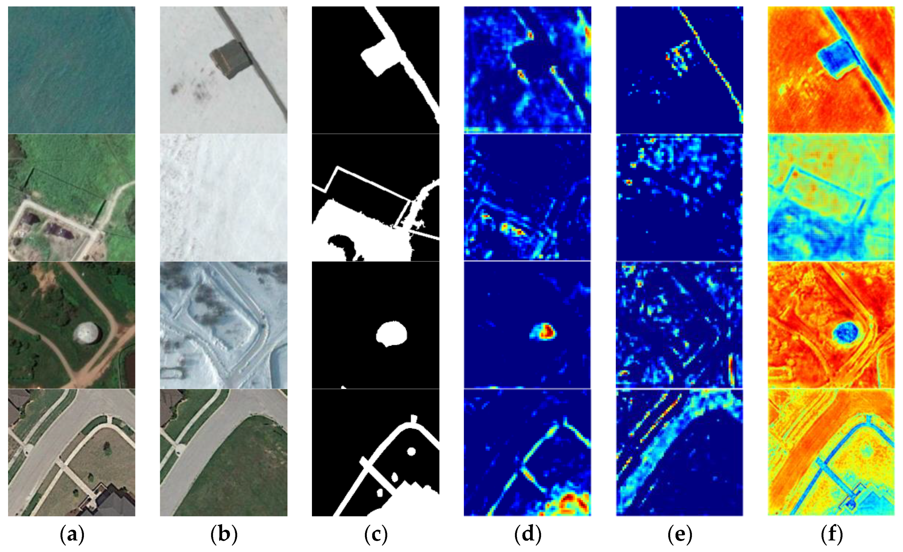
After obtaining the feature sets of the bi-temporal images, they were not fused directly like the current methods but were forwarded into an atrous spatial pyramid cross-attention (ASPCA) module to strengthen the representation ability between feature pairs at the same level. As mentioned above, the ASPCA module was also realized based on self-attention theory shown in Figure 3. The subgraphs in the third column represent the dual spatial features and dual channel features refined by ASPCPA and ASPCCA, respectively. Unlike most attention-based works that forward a concatenated single feature into the attention module and output a single weighted feature, our module utilized dual features without fusing or adding operations.

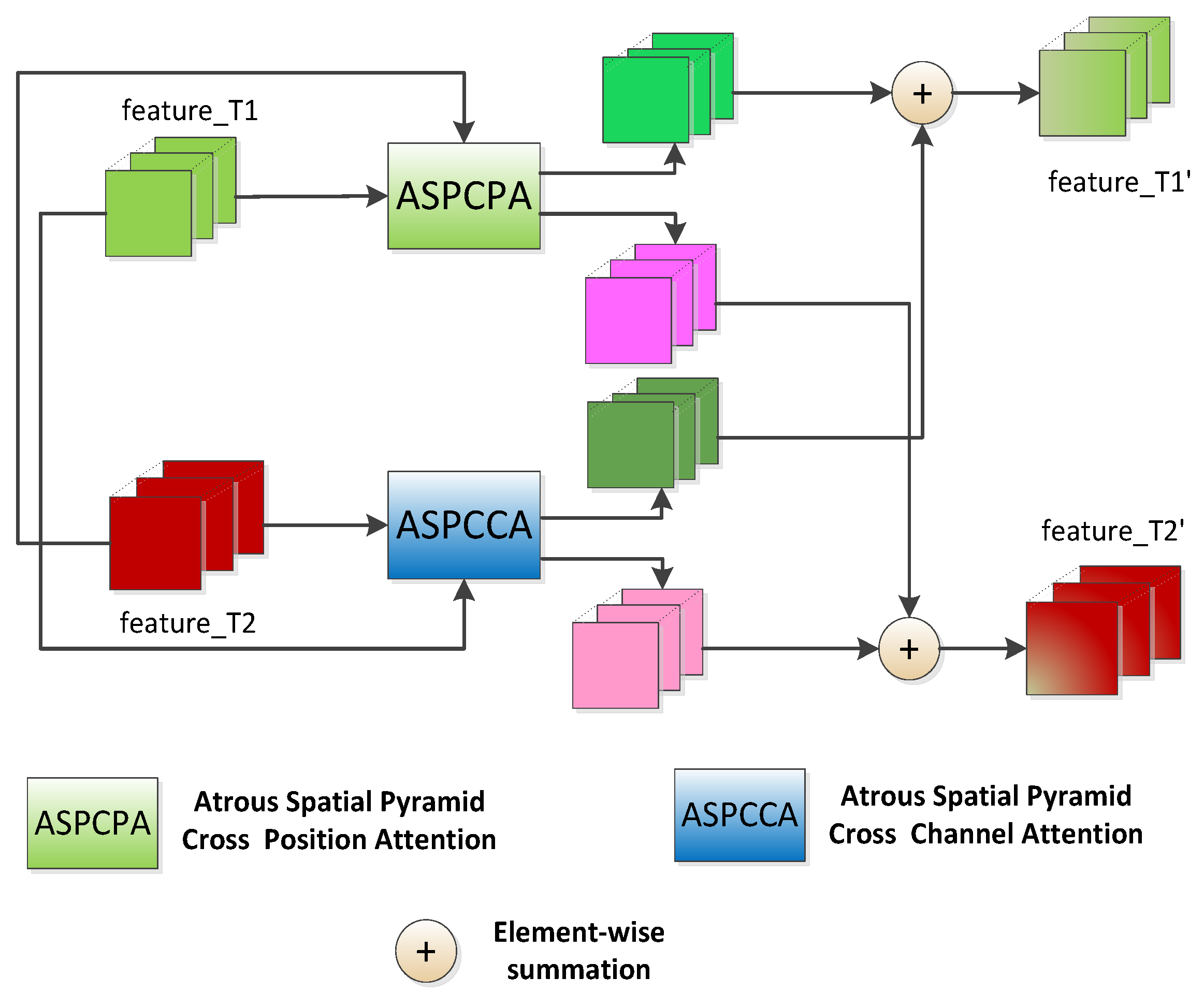
The ASPCA module comprises an atrous spatial pyramid cross-position attention (ASPCPA) module and an atrous spatial pyramid cross-channel attention (ASPCPA) module, both of which accept dual features of the same size from the same level of feature extraction layers. The former captured the long-range spatial–temporal interdependencies, while the latter captured the long-range channel–temporal interdependencies. Although there are many operations to fuse spatial attention features and channel attention features such as concatenating or cascading in parallel, the experiments indicated that they were not suitable for this task, so a summing operation was employed. It is worth noting that the updated image feature of the previous time (expressed as $f^{(1)}{}^{\prime }$) and that the updated image feature of the latter time (expressed as $f^{(2)}{}^{\prime }$) equaled the element-wise summation of the spatial attention feature and channel attention feature in the form of crossover. The mathematical expression is as follows:

$$f^{(1)}{}^{\prime }=f_s^{(1)}+f_c^{(1)},f^{(2)}{}^{\prime }=f_s^{(2)}+f_c^{(2)}$$

(1)

where $f^{(1)}{}^{\prime },f^{(2)}{}^{\prime }$ denote the feature pairs updated by the ASPCA module for a certain layer; $f_s^{(1)},f_s^{(2)}$ denote the output bi-temporal features from the ASPCPA module, and $f_c^{(1)},f_c^{(2)}$ denote the output bi-temporal features from the ASPCCA module.

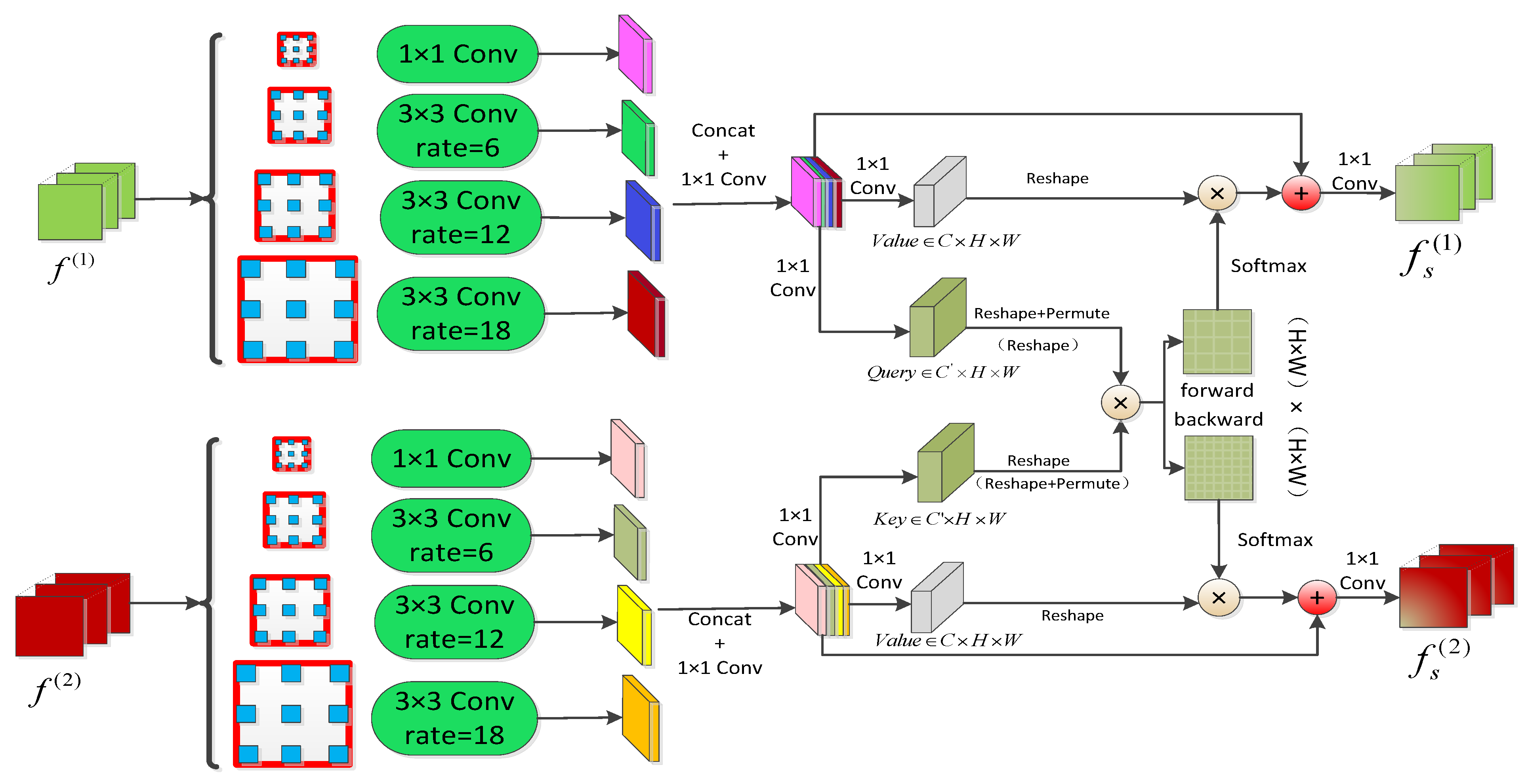
The structure of the ASPCPA module is shown in Figure 4. The green boxes represent the atrous convolution with rates of 1, 6, 12, and 18, respectively and 1 × 1 Conv represents the convolution of kernel size 1 × 1, BatchNorm, and ReLU. We referred to the idea of atrous spatial pyramid pooling (ASPP) in [49]; the dual features were forwarded into an atrous spatial pyramid module containing four atrous convolution operations with ratios of 1, 6, 12, and 18, respectively, and then these output features were concatenated in channel dimension. To increase the nonlinear capability of the model, a convolution with kernel size 1 × 1 operation was performed; we kept the number of channels the same in our work. Given the dual features fused by the atrous spatial pyramid block (denoted as $f_{asp}^{(1)}$ and $f_{asp}^{(2)}$, respectively), where $f_{asp}^{(1)}\in C\times H\times W$ and $f_{asp}^{(2)}\in C\times H\times W$ (C denotes the channel number, and $H\times W$ indicates the spatial size), two parallel $1\times 1$ convolutions were applied to $f_{asp}^{(1)}$ and $f_{asp}^{(2)}$, respectively, which produced $Query\in C^{\prime }\times H\times W$ (expressed as $Q$) and $Key\in C^{\prime }\times H\times W$ (expressed as $K$), where $C^{\prime }$ is the channel number. Generally, $C^{\prime }$ is reduced to 1/4 or 1/8 of $C$ for saving memory, but here we kept them the same. Meanwhile, we forwarded $f_{asp}^{(1)},f_{asp}^{(2)}$ into another two convolution layers to generate corresponding value features $Value\in C\times H\times W$ (expressed as $V_1$ and $V_2$, respectively), which were reshaped into $V_1^{\prime }\in C\times N,V_2^{\prime }\in C\times N$, where $N=H\times W$. Simultaneously, we also reshaped $Q$ and $K$ into $C^{\prime }\times N$. To capture the spatial contextual relationships of feature pairs, we calculated an attention map with forward and backward directions. For the forwarded = direction (“T1 to T2”), $Q$ is permuted to $N\times C^{\prime }$, while $K$ kept the original size; thus, we constructed the forward energy matrix $\mathsf{\Lambda }\in N\times N$, formulated as $\mathsf{\Lambda }=Q^{T}K$, where the element at $(i,j)$ of $\mathsf{\Lambda }$ is the sum product of the $i\mathrm{th}$ row elements of $Q$ and the $j\mathrm{th}$ column elements of $K$ and measures the similarity between $i\mathrm{th}$ position in $f^{(1)}$ and $j\mathrm{th}$ position in $f^{(2)}$. $\mathsf{\Lambda }$ then performed the normalization by Softmax operation and matrix multiplication with $V_1^{\prime }$, as mentioned above, where the former is calculated as follows:

$${\Pi }_{1\to 2}^{(i,j)}=\frac{\exp \left({\mathsf{\Lambda }}^{(i,j)}\right)}{{\displaystyle {\sum }_{j=1}^{N_2}\exp \left({\mathsf{\Lambda }}^{(i,j)}\right)}}$$

(2)

where ${\mathsf{\Lambda }}^{(i,j)}$ indicates the element at position $(i,j)$, and $N_2$ indicates columns of $\mathsf{\Lambda }$. Similar to this, another energy matrix of the backward direction (“T2 to T1”) is formulated as $\mathsf{\Omega }=K^{T}Q$, which means the matrix multiplication of $K$ after transposed and $Q$. We also applied Softmax to $\mathsf{\Omega }$ as follows:

$${\Pi }_{2\to 1}^{(i,j)}=\frac{\exp \left({\mathsf{\Omega }}^{(i,j)}\right)}{{\displaystyle {\sum }_{i=1}^{N_1}\exp \left({\mathsf{\Omega }}^{(i,j)}\right)}}$$

(3)

Slightly different from the above, a backward direction attention map was used to measure the similarity between the $j\mathrm{th}$ position in $f^{(2)}$ and the $i\mathrm{th}$ position in $f^{(1)}$. $N_1$ is the rows of the $\mathsf{\Omega }$ matrix. The bidirectional similarity measurements contributed more comprehensive spatial change context between dual features. Finally, we obtained the updated spatial attention map of $f^{(1)}$ named $f_s^{(1)}$ by adding $f_{asp}^{(1)}$ to the weighted $V_1^{\prime }$:

$$f_s^{(1)}=f_{asp}^{(1)}+\partial V_1^{\prime },$$

(4)

where

$$V_1^{\prime }=V_1{\Pi }_{1\to 2}^{(i,j)}{}^T$$

(5)

and $\partial$ is a model parameter with an initial value of 1, leveraging the dissimilarity importance of $f^{(1)}$ compared to $f^{(2)}$. Conversely, an argument spatial attention map of $f^{(2)}$ named $f_s^{(2)}$ was generated by adding $f_{asp}^{(2)}$ to the weighted $V_2^{\prime }$:

$$f_s^{(2)}=f^{(2)}+\beta V_2^{\prime }$$

(6)

and

$$V_2^{\prime }=V_2{\Pi }_{2\to 1}^{(i,j)}$$

(7)

The model parameter $\beta$ was also initialized to 1, which leverages the dissimilarity importance of $f^{(2)}$ compared to $f^{(1)}$.

In a word, long-range spatial independencies form two directions, both with a strengthened change representation ability for bi-temporal features.

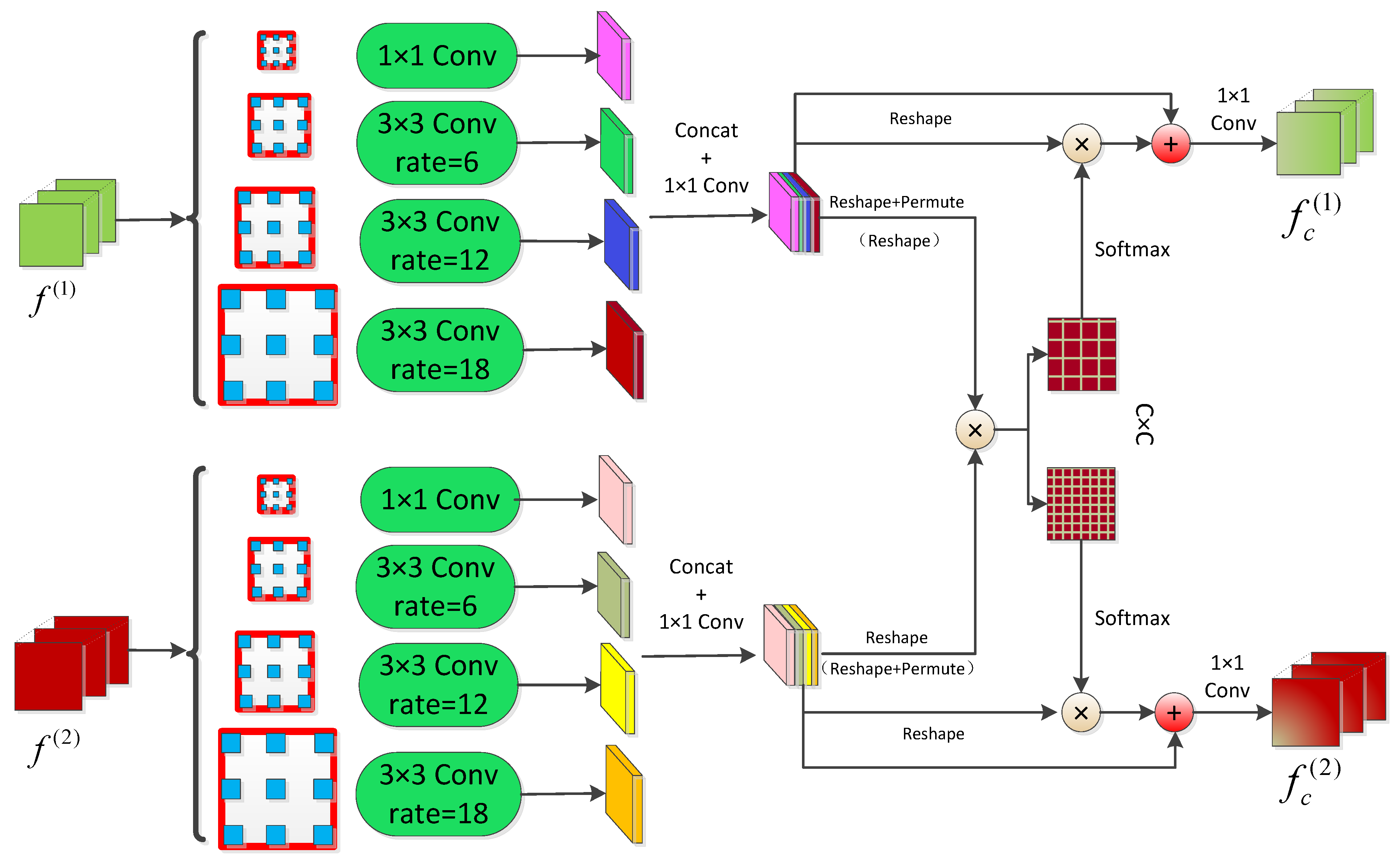
The ASPCCA module was designed to capture long-range channel independencies between $f^{(1)}$ and $f^{(2)}$. As shown in Figure 5, the atrous spatial pyramid and bidirectional structures are identical to ASPCPA except that the latter has to produce $K$, $Q$, $V_1$ and $V_2$ by four 1 × 1 convolution layers before calculating attention maps. Here, we performed matrix multiplication of the original concatenated features directly. Given dual multi-scale features $f_{asp}^{(1)}\in C\times H\times W$ and $f_{asp}^{(2)}\in C\times H\times W$ mapped by four atrous convolutions at rates of 1, 6, 12, and 18, respectively, we reshaped both of them into $C\times N$, where $N=H\times W$. For the forward direction (T1 to T2), the transposed $f_{asp}^{(1)}$ performed matrix multiplication with $f_{asp}^{(2)}$ formulated as $\mathsf{\Phi }=f_{asp}^{(1)}{f}_{asp}^{(2)}{}^T$ to generate forward energy map $\mathsf{\Phi }\in C\times C$. $\mathsf{\Phi }$ was also normalized by a Softmax operation to get an attention map:

$${{\rm T}}_{1\to 2}^{(i,j)}=\frac{\exp \left({\mathsf{\Phi }}^{(i,j)}\right)}{{\displaystyle {\sum }_{j=1}^C\exp \left({\mathsf{\Phi }}^{(i,j)}\right)}}$$

(8)

Finally, the augmented channel attention map of $f^{(1)}$ could be calculated as follows:

$$f_c^{(1)}=f_{asp}^{(1)}+\delta f_{asp}^{(1)}{}^{\prime }$$

(9)

where

$$f_{asp}^{(1)}{}^{\prime }=T_{1\to 2}^{(i,j)}{f}_{asp}^{(1)}$$

(10)

and $\delta$ is a model parameter like $\partial$; here, $f_c^{(1)}$ models the channel context from $f^{(1)}$ to $f^{(2)}$.

In the same way, a backward energy map ${{\rm T}}_{2\to 1}^{(i,j)}$ was calculated by $Y=f_{asp}^{(2)}{f}_{asp}^{(1)}{}^T$ and normalized as follows:

$${{\rm T}}_{2\to 1}^{(i,j)}=\frac{\exp \left(Y^{(i,j)}\right)}{{\displaystyle {\sum }_{j=1}^C\exp \left(Y^{(i,j)}\right)}}$$

(11)

Thereby, the augmented channel attention map of $f^{(2)}$ was obtained:

$$f_c^{(2)}=f_{asp}^{(2)}+\rho f_{asp}^{(2)}{}^{\prime }$$

(12)

where

$$f_{asp}^{(2)}{}^{\prime }=T_{2\to 1}^{(i,j)}{}^T{f}_{asp}^{(2)}$$

(13)

and $\rho$ is a model parameter with an identical initial value like $\delta$; $f_c^{(2)}$ models the channel context from $f^{(2)}$ to $f^{(1)}$.

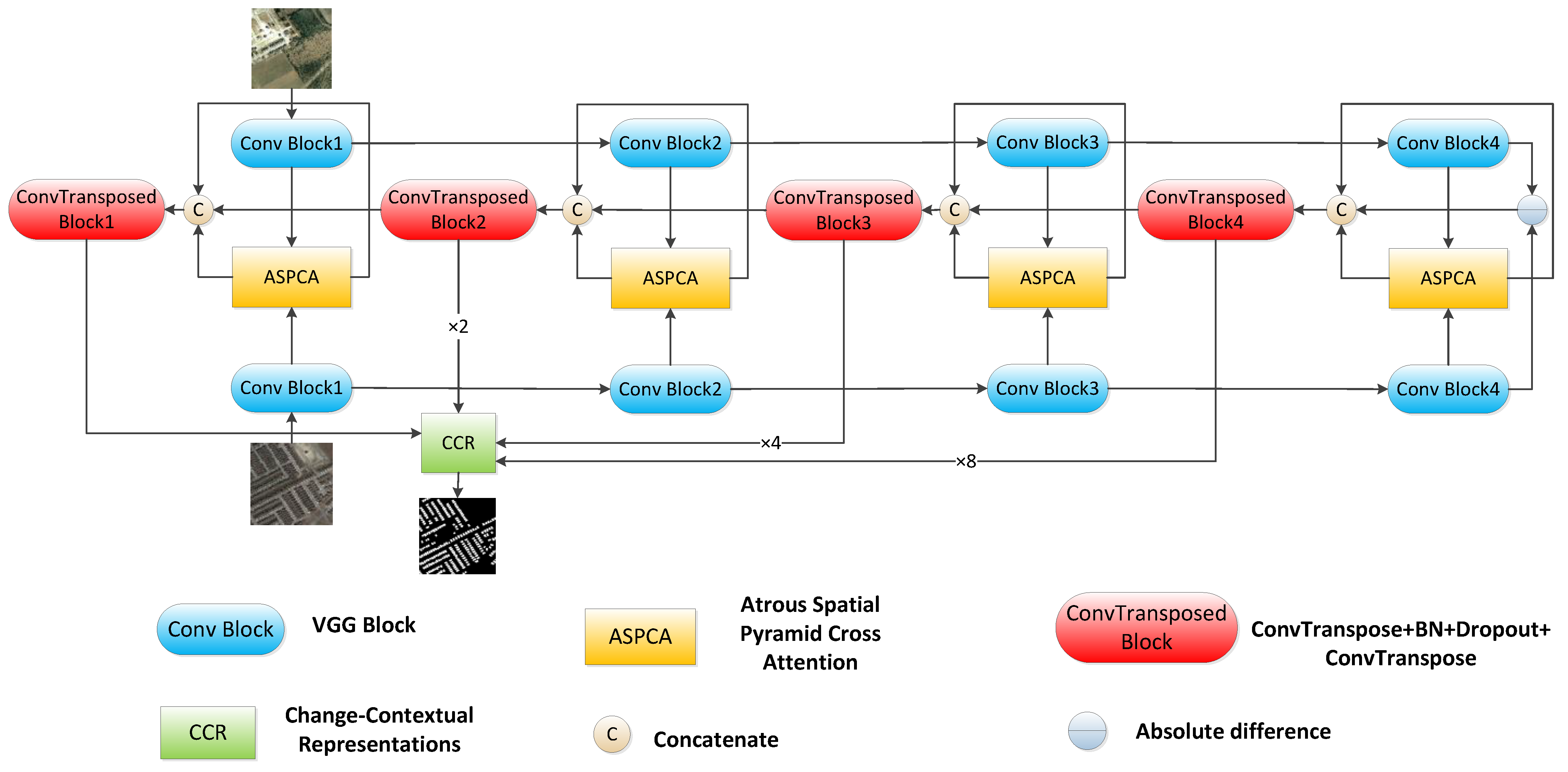
Whether in the ASPCPA module or the ASPCCA module, a norm layer comprising 1 × 1 convolution, BatchNorm, and a ReLU activation function was separately applied to $f_s^{(1)}$, $f_s^{(2)}$, $f_c^{(1)}$, and $f_c^{(2)}$, which ensured that the channel number of the input remains unchanged after being updated by ASPCA. As shown in Figure 2, the decoder gradually restored the change feature map resolution by forwarding concatenated $f^{(1)}{}^{\prime }$, $f^{(2)}{}^{\prime }$ and $abs(f^{(1)}{}^{\prime }-f^{(2)}{}^{\prime })$ (where abs denotes absolute operation) into the upsampling block $ConvTransposed$ from high layers to bottom layers. For each $ConvTransposed$ block, the first two $ConvTransposed2d$ layers are used for dimension reduction, while the other one aims to upsample the doubled spatial size. The specific parameters and feature sizes are shown in

Table 1. The architectural details for our ConvTransposed layers. ConvTransposed2d, BatchNorm2d, and Dropout2d indicate transposed convolution, batch normalization, and dropout operations, respectively; the next subcolumn gives the corresponding parameters.

ConvTransposed Layers	Operations and Parameters		Input Size	Output Size
ConvTransposed Block 4	ConvTransposed2d	3 × 3, stride 1, padding 1	1536 × 16 × 16	1024 × 16 × 16
	BatchNorm2d & Dropout2d	affine true, p 0.2	1024 × 16 × 16
	ConvTransposed2d	3 × 3, stride 1, padding 1	1024 × 16 × 16	512 × 16 × 16
	BatchNorm2d & Dropout2d	affine true, p 0.2	512 × 16 × 16
	ConvTransposed2d	3 × 3, stride 2, padding 1, output_padding 1	512 × 16 × 16	512 × 32 × 32
ConvTransposed Block 3	ConvTransposed2d	3 × 3, stride 1, padding 1	1024 × 32 × 32	512 × 32 × 32
	BatchNorm2d & Dropout2d	affine true, p 0.2	512 × 32 × 32
	ConvTransposed2d	3 × 3, stride 1, padding 1	512 × 32 × 32	256 × 32 × 32
	BatchNorm2d & Dropout2d	affine true, p 0.2	256 × 32 × 32
	ConvTransposed2d	3 × 3, stride 2, padding 1, output_padding 1	256 × 32 × 32	256 × 64 × 64
ConvTransposed Block 2	ConvTransposed2d	3 × 3, stride 1, padding 1	512 × 64 × 64	256 × 64 × 64
	BatchNorm2d & Dropout2d	affine true, p 0.2	256 × 64 × 64
	ConvTransposed2d	3 × 3, stride 1, padding 1	256 × 64 × 64	128 × 64 × 64
	BatchNorm2d & Dropout2d	affine true, p 0.2	128 × 64 × 64
	ConvTransposed2d	3 × 3, stride 2, padding 1, output_padding 1	128 × 64 × 64	128 × 128 × 128
ConvTransposed Block 1	ConvTransposed2d	3 × 3, stride 1, padding 1	256 × 128 × 128	128 × 128 × 128
	BatchNorm2d & Dropout2d	affine true, p 0.2	128 × 128 × 128
	ConvTransposed2d	3 × 3, stride 1, padding 1	128 × 128 × 128	64 × 128 × 128
	BatchNorm2d & Dropout2d	affine true, p 0.2	64 × 128 × 128
	ConvTransposed2d	3 × 3, stride 2, padding 1, output_padding 1	64 × 128 × 128	64 × 256 × 256

.

The multi-scale features up-sampled by the four ConvTransposed blocks contain abundant change discriminatory information with different levels, which means that high layers contain rich abstract semantic information, while low levels represent detailed texture information.

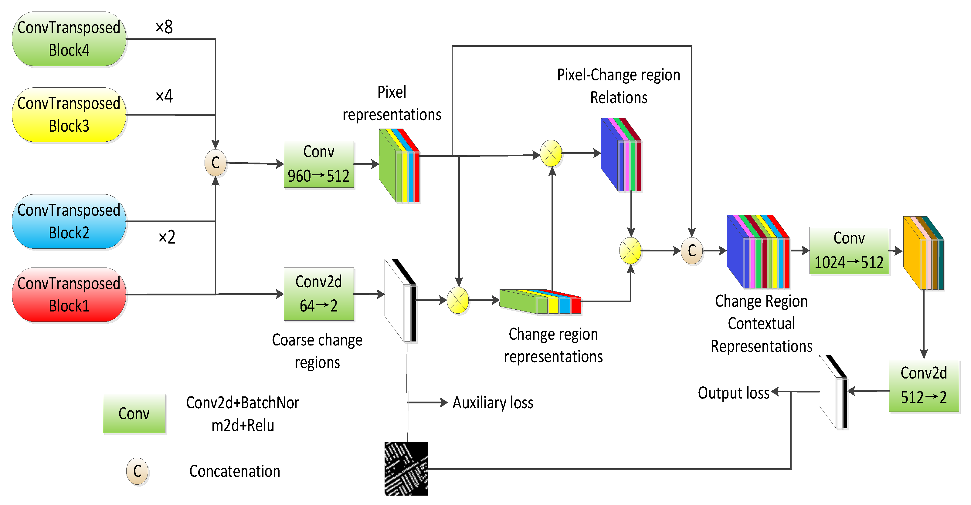
2.1.4. Change Contextual Representational Module

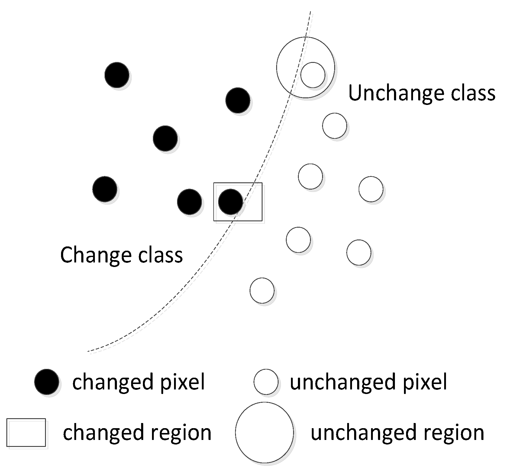
The multi-level features updated by the ASPCA module in Section 2.1.3 only capture the long-range interdependencies between pixels of feature pairs. This subsection proposes a change contextual representational (CCR) module, which captures pixel-change region relation and change region contextual representations by exploiting representations of change regions that the pixels belong to. In Figure 6, ×8, ×4, and ×2 represent bilinear interpolation to 8, 4, and 2 times the original size, respectively, and Conv2d, in the green box, represents a general 1 × 1 convolution while Conv in the green box represents $1\times 1\hspace{0.17em}conv\to BatchNorm\to ReLU$. The features outputted from the four ConvTransposed blocks were resized to be the same as the output from ConvTransposed Block 1, then the fused feature was forwarded into a linear activation layer called Conv to get the pixel representations. Meanwhile, an auxiliary output from a fully convolution layer contributed to the coarse change detection result, which was supervised by an auxiliary loss. Given pixel representations $P\in C\times H\times W$ and coarse change regions $O\in 2\times H\times W$, where 2 indicates the change class and unchanged class, both $P$ and $O$ were separately reshaped to $P^{\prime }\in C\times N$ (to reduce calculation complexity, $C$ means 512 in this work) and $O^{\prime }\in 2\times N$. Then the change region representations $f_c\in C\times 2$ could be obtained by a matrix multiplication between regularized $O^{\prime }$ and $P^{\prime }$ formulated as follows:

$$f_c={(softmax(O^{\prime }{}^T)P^{\prime })}^T$$

(14)

Similar to the attention map in ASPCA, the pixel-change region relation $f_{att}$ was calculated by:

$$f_{att}=softmax(\sigma {(f_c)}^T\varphi (P^{\prime }))$$

(15)

where $\sigma$ and $\varphi$ were both implemented as $1\times 1\hspace{0.17em}conv\to BatchNorm\to ReLU$ and $f_{att}\in 2\times N$. Then the matrix multiplication of change region representations $f_c$ and attention map $f_{att}$. were calculated as follows:

$$f_{context}=\rho (\delta (f_c)f_{att}),$$

(16)

where $\delta$ and $\rho$ are also transform functions like $\sigma$ and $\varphi$, but it is worth noting that $\sigma$, $\varphi$, and $\delta$ are all dimension reduction transformation (512 to 256 in this work), while $\rho$ denotes $1\times 1\hspace{0.17em}conv$ from 256 channel to 512. For reusing the pixel representations, $f_{context}$ was first reshaped to $f_{context}^{\prime }\in C\times H\times W$ and then concatenated with $P$ to generate change region contextual representations, updated by a Conv layer to restore the original channel dimensions. Finally, a pixel-level convolution predicted the change intensity map.

2.2. Datasets

In this work, we experimented with four public remote sensing image change detection datasets of different resolutions, namely LEVIR-CD [9], Season-Varying Change Detection Dataset (CCD) [7], Google Data GZ [50], and DSIFN [10].

The attributes are shown in

Table 2. Datasets’ attributes. VHR indicates very high resolution.

Datasets	Resolution (m/Pixel)	Scale (Pixel)	Type	Training:Validation:Testing
LEVIR-CD	0.5	1024 × 1024	VHR	445:64:128
CCD	0.03–0.1	256 × 256	Low-resolution	10,000:3000:3000
Google Data GZ	0.55	4936 × 5224	VHR	9:6:4
DSIFN	2	512 × 512	VHR	3600:340:48

. The LEVIR-CD dataset contains 637 very-high-resolution Google Earth (GE) image patch pairs with a size of 1024 × 1024 pixels, covering 20 different regions in Texas, USA. Most image pairs belonging to building change involve man-made structures and date from 2002 to 2018. The Season-Varying Change Detection Dataset (CCD) also originated from Google Earth but the spatial resolution ranges from 3 to 100 cm/pixel. Different from the first one, this dataset is more focused on changes corresponding to the appearance and disappearance of objects, but ignores changes due to seasonal differences, brightness, and other factors. Google Data GZ is a large-scale VHR change detection satellite image dataset obtained from 2006 to 2019, covering suburban areas of Guangzhou City, China. Google Data GZ contains 19 season-varying VHR images pairs with three bands, which mainly focus on building changes. The last DSIFN dataset is collected from Google Earth, covering many Chinese cities such as Beijing, Chengdu, Shenzhen, Chongqing, Wuhan, etc. In the training stage, all datasets were cropped into 256 × 256 patches.

2.3. Loss Design

To solve the sample class-imbalanced problem in change detection, we proposed an effective sample number adaptively weighted loss. The point of this is to associate each sample with a small neighboring region instead of a single point. From [37], it can be realized that a newly sampled pixel either inside a previously sampled changed region with the probability of p or an outside, unchanged region with the probability of 1 − p, which means the effective number of samples is the expected volume of samples, so the loss was designed to capture the hidden marginal benefits by using more data points of a class. Following the mathematical formulation of effective number, the effective sample number adaptively weighted loss (EAWLoss) was defined as follows:

$$L_{EAW}(y,\hat{y})=\{\begin{array}{c}\frac{1-\beta }{1-{\beta }^{n_1}}L(y,\hat{y}),\hspace{1em}y=1\\ \frac{1-\beta }{1-{\beta }^{n_0}}L(y,\hat{y}),\hspace{1em}y=0\end{array}$$

(17)

where $n_1$ and $n_0$ indicate the number of changed pixels and unchanged pixels in ground truth, respectively; $L(y,\hat{y})$ represents the standard cross entropy loss or focal loss [51] between the label and the predicted result. $\beta$ controls the proportion of effective sample number; in this work, it was set to 0.5 as the change detection task only contains two classes, where $\beta =0$ means no reweighting and $\beta \to 1$ means reweighting by inverse class frequency. To keep the experiments identical, we also used EAWLoss as the auxiliary supervision loss. So, the total loss was expressed as follows:

$$L_{sum}(y,{\hat{y}}_{out},{\hat{y}}_{aux})=L_{EAW}(y,{\hat{y}}_{out})+\lambda L_{EAW}(y,{\hat{y}}_{aux})$$

(18)

where $y,{\hat{y}}_{out},{\hat{y}}_{aux}$ are ground truth, final prediction, and auxiliary prediction, and $\lambda$ is the weight factor and was set to 0.4.

2.4. Implementation Details

To verify the effectiveness of the proposed method, five evaluation metrics were utilized to quantify the experiment’s performance, defined in Section 2.4.1. The training details of the experiments and model configuration are given in Section 2.4.2.

2.4.1. Evaluation Metrics

In this work, we utilized overall accuracy (OA), mean intersection over union (mIoU), precision (precision), recall (recall), and F1-score (F1) as performance metrics, the definitions of which are as follows:

$$OA=\frac{TP+TN}{TP+FP+TN+FN}$$

(19)

$$mIOU=\frac{TP}{FP+FN+TP}$$

(20)

$$Precision=\frac{TP}{TP+FP}$$

(21)

$$Recall=\frac{TP}{TP+FN}$$

(22)

$$F1=\frac{2\cdot Precision\cdot Recall}{Precision+Recall}$$

(23)

where true positive (TP) indicates the number of pixels predicted correctly as changed; true negative (TN) represents the number of pixels predicted correctly as unchanged; false positive (FP) denotes the number of pixels predicted incorrectly as changed, and false negative (FN) means the number of pixels predicted incorrectly as unchanged. Generally, high precision or high recall is only suitable for specific applications. F1 combines the characteristics of the two measurements, creating a benchmark.

2.4.2. Experiment Details

Our work was implemented by PyTorch with two Telsa GPUs with 12 GB memory. In the training phase, we cropped the image pairs of the above datasets into 256 × 256 nonoverlapping patches before forwarding them to the model. The VGG16 backbone of the model was initialized with an ImageNet-pretrained [52] weight, and the initial learning rate was 0.0001. We chose cosine annealing as the learning rate decay mode. The value decreased slowly during the first 50 epochs, then increased over the next 50 epochs. Adam solver was used [53] as the model optimizer with ${\beta }_1=0.5$ and ${\beta }_2=0.99$. Random crop, random flip, and random rotation from −30° to 30° were utilized to increase the generalization of the model.

3. Results

In this section, we present quantitative comparisons and visualization results of our method. The ablation experiment results are described in Section 3.1. The evaluation metric comparison with other related methods is given in Section 3.2.

3.1. Ablation Study

To assess the effectiveness of the proposed ASPCA module and the CCR module, we experimented with different modules, comparing them to the baseline on CCD dataset. Specifically, the baseline was built without any attention module, but a basic encoder–decoder structure, including a VGG16 backbone and four ConvTransposed blocks. In addition, the effective sample number adaptively weighted loss was compared with usual cross entropy loss. All the experiments show that our ASPCA module, the CCR module, and loss improved the performance. The complete ablation results are shown in

Table 3. Ablation study of different modules on CCD dataset. The bold type indicates the best results.

Method	Precision	Recall	F1	mIOU	OA
Baseline	97.25	89.47	93.20	92.68	98.42
+ASPCA	97.36	91.39	94.28	94.22	98.67
+CCR	97.46	93.92	95.66	95.34	98.96
+ASPCA + CCR	97.52	95.32	96.41	96.07	99.25

.

Compared to the baseline, we outperformed 0.49 points of the F1-score and 1.04 points of the mean intersection over union with only the ASPCA module, while the CCR module outperformed by 1.95 points the F1-score and by 2.16 points the mean intersection over union. The combination of both proposed modules achieved the best results, as seen in the last row of Table 3: it outperformed by 3.19 points the F1-score and by 2.74 points the mean intersection over union. The visual comparison results of the ablation experiment are shown in Figure 7, wherein black indicates unchanged pixels predicted correctly and white indicates changed pixels predicted correctly. Red indicates unchanged pixels predicted in error, and green indicates ignored changed pixels. The ASPCA module slightly improved the ability to capture the interdependencies of pixels, thus migrating the holes in enormous areas. The CCR module strongly corrected pixels predicted in error compared to the baseline and preferred to continuously refine for specific shapes or texture regions. The model with both modules had the best performance and effectively solved the problem of ignored change pixels.

Our designed loss is also crucial for the experiment’s performance.

Table 4. Ablation study of proposed loss on CCD dataset. CE means cross-entropy loss. The bold type indicates the best result.

Method	F1
Baseline (with CE)	92.42
Baseline (with EAW)	93.71
+ASPCA (with CE)	92.17
+ASPCA (with EAW)	94.28
+CCR (with CE)	93.88
+CCR (with EAW)	95.66
+ASPCA + CCR (with CE)	94.59
+ASPCA + CCR (with EAW)	96.41

gives the ablation study of our proposed effective sample number adaptively weighted loss (EAWLoss) on the CCD dataset.

For each item, the performance with EAWLoss was better than the cross-entropy loss. The visual ablation result is shown in Figure 8. To further verify the robustness of our method, we listed the results of different scenarios. The first four columns in Figure 8 are based on large buildings or roads, and the latter four are based on small vehicles. It can be seen that our designed EAWLoss effectively solved the class-imbalanced problem.

To measure the computational efficiency of the proposed model, the comparisons of GFLOPs and parameter size are given in

Table 5. Comparisons of computational efficiency.

	GFLOPs (G)	Parameters (M)
Baseline	410.97	42.88
+ASPCA	438.80	62.42
+CCR	436.56	43.00
+ASPCA + CCR	464.39	62.55

. As can be seen, the proposed modules improved the performance while modestly increasing the computational complexity.

3.2. Comparisons with Other Methods

We experimented on the four datasets described in Section 2.2 to compare our method with recent learning-based change detection methods:

• FC-EF [6]: Image-level fusing method based on FCN: concatenating the bi-temporal images as the model input and transferring the feature information by a skip-connection from the encoder to the decoder.
• FC-Siam-conc [6]: Single-level feature fusing method based on FCN, which employed a Siamese encoder–decoder structure for the inputting of bi-temporal images. In the decoder, this involves concatenating the upsampled feature with dual features extracted by the encoder to gradually restore the changed map resolution.
• FC-Siam-diff [6]: Single-level fusing method based on FCN, which used Siamese structure for bi-temporal input. The only difference from FC-Siam-conc is that the skip -connection was replaced by the absolute difference rather than the element-wise sum of feature maps.
• U-Net++ [7]: An image-level fusing method based on U-Net++ [44], which utilized deep supervision by multiple side-outputs fusion of concatenated bi-temporal images.
• DASNet [27]: A dual-branch, metric-based method based on spatial attention and channel attention mechanism, which aimed to punish the L2 distance between feature pairs updated by the dual attention module, thus making the changed pair and unchanged pair more easily discriminated.
• STANet [9]: A single-level feature fusing method based on distance metric, which employed a spatial–temporal attention module to capture the temporal–spatial dependency between the bi-temporal images.
• SNUNet-CD [54]: A feature-level, densely connected Siamese method based on U-Net++, which mitigates localization information loss in the deep layers by transmitting compact information from the encoder to the decoder. Moreover, an ensemble channel attention module is proposed to aggregate and refine features of multiple semantic levels.

We experimented with the above methods according to the original parameters described in corresponding papers.

Table 6. Comparison of results on the LEVIR-CD dataset. The bold numbers indicate the best results.

Method	Precision	Recall	F1	mIOU	OA
FC-EF	81.26	80.17	80.71	71.53	98.39
FC-Siam-conc	91.99	76.77	83.69	71.96	98.49
FC-Siam-diff	89.64	82.68	86.02	78.86	98.65
U-Net++	90.66	85.32	87.91	80.94	98.24
DASNet	80.76	79.53	79.91	78.65	94.32
STANet	83.81	91.02	87.27	78.64	98.87
SNUNet	91.85	88.69	90.24	82.21	98.11
MCCRNet (ours)	89.91	89.62	90.71	91.13	99.24

reports the quantitative comparison results on the LEVIR-CD dataset. For F1 score, mIOU, and OA, our model outperformed other learning-based methods. The visualization is shown in Figure 9; due to the first three models being similar, only the visual map produced by FC-Siam-conc was listed.

The quantitative comparison result on the CCD dataset is shown in

Table 7. Comparison of results on the CCD dataset. The bold numbers indicate the best results.

Method	Precision	Recall	F1	mIOU	OA
FC-EF	60.63	57.42	58.98	46.64	88.49
FC-Siam-conc	68.96	59.33	63.78	50.66	90.33
FC-Siam-diff	76.84	64.33	70.03	52.44	89.69
U-Net++	89.54	87.10	88.30	84.58	96.88
DASNet	91.28	86.34	88.74	80.94	96.98
STANet	95.88	94.69	95.28	94.44	98.35
SNUNet	96.32	96.28	96.30	95.48	99.04
MCCRNet (ours)	97.52	95.32	96.41	96.07	99.25

. Our model also outperformed the other methods in terms of precision, F1, mIOU, and OA; in particular, the precision achieved quite a high level.

The visualization of the ablation results is shown in Figure 10. We still only give the results of FC-Siam-conc for the fully convolutional network (the first three items in Table 7). It can be seen that, whether the change scene is small vehicles or broad roads, our method greatly reduces the ignored area (the green parts in Figure 10) and further corrects the mispredicted unchanged pixels (the red parts in Figure 10).

A comparison between different methods is shown in

Table 8. Comparison results on Google Data GZ dataset. The bold numbers indicate the best results.

Method	Precision	Recall	F1	mIOU	OA
FC-EF	85.47	76.58	80.78	74.26	96.64
FC-Siam-conc	87.22	78.44	82.60	75.32	96.98
FC-Siam-diff	87.43	78.51	82.36	75.20	96.48
U-Net++	88.10	78.64	83.10	76.23	97.26
DASNet	82.38	81.94	82.16	83.04	96.59
STANet	90.02	87.61	88.80	88.59	97.72
SNUNet	88.47	90.02	89.27	89.12	97.83
MCCRNet (ours)	90.18	93.66	91.89	91.58	98.32

, from which we achieved state-of-the-art on all metrics, and the F1 and OA were much higher than the semi-supervised methods.

The visual comparison results are shown in Figure 11. For most change regions of buildings, our model effectively migrated the gaps between discontinuous blocks and refined the building edges.

We also give the quantitative comparison results on DSIFN dataset in

Table 9. Comparison of results on DSIFN dataset. The bold numbers indicate the best results.

Method	Precision	Recall	F1	mIOU	OA
FC-EF	70.38	51.69	56.60	43.95	84.68
FC-Siam-conc	62.54	56.39	59.31	42.48	86.34
FC-Siam-diff	58.66	64.38	61.39	44.46	85.78
U-Net++	60.42	66.88	63.49	46.33	86.68
DASNet	53.87	74.68	68.42	47.74	84.92
STANet	67.68	61.36	64.36	47.48	88.59
SNUNet	69.97	75.66	72.70	49.68	89.22
MCCRNet (ours)	66.12	91.28	76.69	67.08	81.69

. Due to the high resolution and the complex environment, most of the methods could not achieve excellent performance, but MCCRNet achieved a remarkable result for recall.

The visualization of comparison results is shown in Figure 12. Our method greatly reduced the change regions ignored by the network (the green parts in Figure 12).

4. Discussion

Our study aimed to obtain the change map of bi-temporal remote sensing images from the perspective of two points: dual long-range interdependencies between feature pairs and change region contextual representation. In addition, we achieved a coarse-to-fine change detection network by employing multi-scale feature pairs rather than a single-level fused feature. The proposed ASPCA module adopted an atrous spatial pyramid pooling structure and a dual self-attention mechanism to capture bi-directional attention maps, effectively strengthening the distinguishable change information between feature pairs. From the ablation study in Section 3.1, we found that the ASPCA module could improve the performance of change detection. The change contextual representational module utilized the relationship between pixels and their contextual region to correct misclassified pixels, especially for those changed pixels that were predicted to be unchanged (false negatives). The CCR module first introduced the class mechanism into the change detection task.

4.1. The Effectiveness of ASPCA

To verify the capacity of strengthening feature pairs’ representation with the ASPCA module, we created visualization heatmaps of features updated by ASPCA module, as shown in Figure 13. Due to the low resolution of high-level features, only the feature pair from the last ASPCA (named att1_1 and att1_2) and the fused one from ConvTransposed Block 1 (named transconv1) are given. From this, ASPCA enhanced the distinguishable differences of dual features by applying interactive attention weights. Different from other change detection methods based on attention mechanism, ASPCA receives two inputs corresponding to bi-temporal features and produces dual-features output, avoiding the defects of single-feature representation. In particular, the bottom layers (such as layer 1 and layer 2) in the encoder tend to extract more detailed texture information, while high layers (such as layer 3 and layer 4) extract more abstract semantic information, so the former emphasizes more detailed change appearance information such as edges, shapes, and colors, while the latter emphasizes global change semantic information such as categories and regions.

4.2. The Effectiveness of CCR

To verify the capacity of correcting misclassified pixels, the feature maps output from the CCR module were was visualized. As shown in Figure 14, we made an attention map of pixel-change region relationships and the heatmap of change region contextual representations. As can be seen, the region around the change pixels most likely belongs to the same change category, which indicates that the change region representations are weighted by pixel-change region relationships, thus producing finer change region contextual representations. In this work, the channel of fused feature was reduced from 960 to 512, thus decreasing the computational cost and simultaneously increasing the nonlinear ability.

In addition, we adopted an auxiliary supervision with the last upsampled feature to increase the generalization ability in the training stage, but it was removed in the testing stage.

4.3. Generalization

As the experiments show, datasets with different resolutions had varying generalization abilities: VHR image pairs were harder to distinguish due to elaborate object details, while low-resolution samples gained a more gratifying results owing to a task-surpassed network model. Specifically, our model obtained finer building outlines for the LEVIR dataset and had stronger generalizability in season-varying change scenes. For the CCD dataset, the model learned excellent discriminable weights from season-varying image pairs, including objects of different scales (such as cars and buildings). As the results of DSIFN present, image pairs with sophisticated and multi-view circumstances had greatly reduced performance due to the prominent depth difference. For common grounds, all datasets were sensitive to object edges, caused by intrinsic defects of cascading transposed convolutions.

5. Conclusions

In this work, we have proposed an end-to-end network named a multi-level change contextual refinement network (MCCRNet) for remote sensing image change detection. The MCCRNet creatively put forward a dual-input and dual-output attention module ASPCA. A CCR module first introduced a corrective ability for mispredicted pixels in the manner of coarse-to-fine. In addition, we designed a novel loss to solve the class-imbalanced problem based on cost-sensitive learning. Compared to early methods, our loss adaptively adjusted the weight of positive and negative samples’ loss with an increase in the number of training iterations. As to the overall structure of the proposed network, multi-level dual features were fully fused in a cascade manner, thus helping to discriminate change representations. The experimental results on four change datasets proved the validity of our method. In particular, for low-resolution samples such as the CCD dataset and fine-grained very-high-resolution images such as the LEVIR dataset, our method achieved extremely high performance. On the other hand, our model had a poor generalization ability under the scene of view-changes. So, the image depth will be considered to improve the performance afterwards. In the whole work, a large number of image labels were used for supervised learning, creating labor-intensive and time-consuming challenges for other label-free datasets. In the next stage, we will focus on unsupervised learning to solve change detection tasks.

References

1. Shi, W.; Zhang, M.; Zhang, R.; Chen, S.; Zhan, Z. Change Detection Based on Artificial Intelligence: State-of-the-Art and Challenges. Remote Sens. 2020, 12, 1688. [Google Scholar] [CrossRef]
2. You, Y.; Cao, J.; Zhou, W. A Survey of Change Detection Methods Based on Remote Sensing Images for Multi-Source and Multi-Objective Scenarios. Remote Sens. 2020, 12, 2460. [Google Scholar] [CrossRef]
3. Johnson, R.D.; Kasischke, E.S. Change vector analysis: A technique for the multispectral monitoring of land cover and condition. Int. J. Remote Sens. 1998, 16, 411. [Google Scholar] [CrossRef]
4. Liu, W.; Yang, J.; Zhao, J.; Shi, H.; Yang, L. An unsupervised change detection method using time-series of PolSAR images from radarsat-2 and gaofen-3. Sensors 2018, 18, 559. [Google Scholar] [CrossRef] [PubMed] [Green Version]
5. Wang, X.; Liu, S.; Du, P.; Liang, H.; Xia, J.; Li, Y. Object-based change detection in urban areas from high spatial resolution images based on multiple features and ensemble learning. Remote Sens. 2018, 10, 276. [Google Scholar] [CrossRef] [Green Version]
6. Daudt Caye, R.; Le Saux, B.; Boulch, A. Fully convolutional siamese networks for change detection. In Proceedings of the 2018 25th IEEE International Conference on Image Processing (ICIP), Athens, Greece, 7–10 October 2018. [Google Scholar]
7. Peng, D.; Zhang, Y.; Guan, H. End-to-end change detection for high resolution satellite images using improved UNet++. Remote Sens. 2019, 11, 1382. [Google Scholar] [CrossRef] [Green Version]
8. Fang, B.; Pan, L.; Kou, R. Dual learning-based siamese framework for change detection using bi-temporal VHR optical remote sensing images. Remote Sens. 2019, 11, 1292. [Google Scholar] [CrossRef] [Green Version]
9. Chen, H.; Shi, Z. A spatial-temporal attention-based method and a new dataset for remote sensing image change detection. Remote Sens. 2020, 12, 1662. [Google Scholar] [CrossRef]
10. Zhang, C.; Yue, P.; Tapete, D.; Jiang, L.; Shangguan, B.; Huang, L.; Liu, G. A deeply supervised image fusion network for change detection in high resolution bi-temporal remote sensing images. ISPRS J. Photogramm. Remote Sens. 2020, 166, 183–200. [Google Scholar] [CrossRef]
11. Liu, J.; Gong, M.; Qin, K.; Zhang, P. A deep convolutional coupling network for change detection based on heterogeneous optical and radar images. IEEE Trans. Neural Netw. Learn. Syst. 2016, 29, 545–559. [Google Scholar] [CrossRef] [PubMed]
12. Liu, J.; Chen, K.; Xu, G.; Sun, X.; Yan, M.; Diao, W.; Han, H. Convolutional neural network-based transfer learning for optical aerial images change detection. IEEE Geosci. Remote Sens. Lett. 2019, 17, 127–131. [Google Scholar] [CrossRef]
13. Zhang, M.; Xu, G.; Chen, K.; Yan, M.; Sun, X. Triplet-based semantic relation learning for aerial remote sensing image change detection. IEEE Geosci. Remote Sens. Lett. 2018, 16, 266–270. [Google Scholar] [CrossRef]
14. Wang, M.; Tan, K.; Jia, X.; Wang, X.; Chen, Y. A deep siamese network with hybrid convolutional feature extraction module for change detection based on multi-sensor remote sensing images. Remote Sens. 2020, 12, 205. [Google Scholar] [CrossRef] [Green Version]
15. Mou, L.; Bruzzone, L.; Zhu, X.X. Learning spectral-spatial-temporal features via a recurrent convolutional neural network for change detection in multispectral imagery. IEEE Trans. Geosci. Remote Sens. 2018, 57, 924–935. [Google Scholar] [CrossRef] [Green Version]
16. Bao, T.; Fu, C.; Fang, T.; Huo, H. PPCNET: A Combined Patch-Level and Pixel-Level End-to-End Deep Network for High-Resolution Remote Sensing Image Change Detection. IEEE Geosci. Remote Sens. Lett. 2020, 17, 1797–1801. [Google Scholar] [CrossRef]
17. Wiratama, W.; Lee, J.; Park, S.-E.; Sim, D. Dual-dense convolution network for change detection of high-resolution panchromatic imagery. Appl. Sci. 2018, 8, 1785. [Google Scholar] [CrossRef] [Green Version]
18. Zhang, C.; Wei, S.; Ji, S.; Lu, M. Detecting large-scale urban land cover changes from very high resolution remote sensing images using CNN-based classification. ISPRS Int. J. Geo-Inf. 2019, 8, 189. [Google Scholar] [CrossRef] [Green Version]
19. Deng, Z.; Sun, H.; Zhou, S.; Zhao, J.; Lei, L.; Zou, H. Multi-scale object detection in remote sensing imagery with convolutional neural networks. ISPRS J. Photogramm. Remote Sens. 2018, 145, 3–22. [Google Scholar] [CrossRef]
20. Chen, H.; Wu, C.; Du, B.; Zhang, L.; Wang, L. Change detection in multisource VHR images via deep Siamese convolutional multiple-layers recurrent neural network. IEEE Trans. Geosci. Remote Sens. 2019, 58, 2848–2864. [Google Scholar] [CrossRef]
21. Liu, R.; Cheng, Z.; Zhang, L.; Li, J. Remote sensing image change detection based on information transmission and attention mechanism. IEEE Access 2019, 7, 156349–156359. [Google Scholar] [CrossRef]
22. Ji, S.; Shen, Y.; Lu, M.; Zhang, Y. Building instance change detection from large-scale aerial images using convolutional neural networks and simulated samples. Remote Sens. 2019, 11, 1343. [Google Scholar] [CrossRef] [Green Version]
23. Chen, J.; Yuan, Z.; Peng, J.; Chen, L.; Huang, H.; Zhu, J.; Liu, Y.; Li, H. DASNet: Dual attentive fully convolutional siamese networks for change detection of high resolution satellite images. IEEE J. Sel. Top. Appl. Earth Obs. Remote Sens. 2020, 14, 1194–1206. [Google Scholar] [CrossRef]
24. Jiang, H.; Hu, X.; Li, K.; Zhang, J.; Gong, J.; Zhang, M. Pga-siamnet: Pyramid feature-based attention-guided siamese network for remote sensing orthoimagery building change detection. Remote Sens. 2020, 12, 484. [Google Scholar] [CrossRef] [Green Version]
25. Liu, Y.; Pang, C.; Zhan, Z.; Zhang, X.; Yang, X. Building Change Detection for Remote Sensing Images Using a Dual-Task Constrained Deep Siamese Convolutional Network Model. IEEE Geosci. Remote Sens. Lett. 2020, 18, 811–815. [Google Scholar] [CrossRef]
26. Zhou, Z.; Siddiquee, M.M.R.; Tajbakhsh, N.; Liang, J. Unet++: A nested u-net architecture for medical image segmentation. In Deep Learning in Medical Image Analysis and Multimodal Learning for Clinical Decision Support; Springer: Cham, Switzerland, 2018; pp. 3–11. [Google Scholar]
27. Zhang, X.; Yue, Y.; Gao, W.; Yu, S.; Su, Q.; Yin, H.; Zhang, Y. DifUnet++: A Satellite Images Change Detection Network Based on Unet++ and Differential Pyramid. IEEE Geosci. Remote Sens. Lett. 2021, 1–5. [Google Scholar] [CrossRef]
28. Hu, J.; Li, S.; Gang, S. Squeeze-and-excitation networks. In Proceedings of the IEEE Conference on Computer Vision and Pattern Recognition, Salt Lake City, UT, USA, 18–22 June 2018. [Google Scholar]
29. Wang, X.; Girshick, R.; Gupta, A.; He, K. Non-local neural networks. In Proceedings of the IEEE Conference on Computer Vision and Pattern Recognition, Salt Lake City, UT, USA, 18–22 June 2018. [Google Scholar]
30. Fu, J.; Liu, J.; Tian, H.; Li, Y.; Bao, Y.; Fang, Z.; Lu, H. Dual attention network for scene segmentation. In Proceedings of the IEEE/CVF Conference on Computer Vision and Pattern Recognition, Long Beach, CA, USA, 15–20 June 2019. [Google Scholar]
31. Zhang, F.; Chen, Y.; Li, Z.; Hong, Z.; Liu, J.; Ma, F.; Han, J.; Ding, E. Acfnet: Attentional class feature network for semantic segmentation. In Proceedings of the IEEE/CVF Conference on Computer Vision and Pattern Recognition, Long Beach, CA, USA, 15–20 June 2019. [Google Scholar]
32. Simonyan, K.; Zisserman, A. Very deep convolutional networks for large-scale image recognition. arXiv 2014, arXiv:1409.1556. [Google Scholar]
33. Chen, L.-C.; Papandreou, G.; Schroff, F.; Adam, H. Rethinking atrous convolution for semantic image segmentation. arXiv 2017, arXiv:1706.05587. [Google Scholar]
34. Fernández, A.; García, S.; Galar, M.; Prati, R.C.; Krawczyk, B.; Herrera, F. Cost-sensitive learning. In Learning from Imbalanced Data Sets; Springer: Cham, Switzerland, 2018; pp. 63–78. [Google Scholar]
35. Zhang, C.; Tan, K.C.; Li, H.; Hong, G.S. A cost-sensitive deep belief network for imbalanced classification. IEEE Trans. Neural Netw. Learn. Syst. 2018, 1, 109–122. [Google Scholar] [CrossRef] [PubMed] [Green Version]
36. Khan, A.; Khan, F.; Khan, S.; Khan, I.A.; Saeed, M. Cost Sensitive Learning and SMOTE Methods for Imbalanced Data. J. Appl. Emerg. Sci. 2018, 8, 32–38. [Google Scholar]
37. Cui, Y.; Jia, M.; Lin, T.Y.; Song, Y.; Belongie, S. Class-balanced loss based on effective number of samples. In Proceedings of the IEEE/CVF Conference on Computer Vision and Pattern Recognition, Long Beach, CA, USA, 15–20 June 2019. [Google Scholar]
38. Yang, K.; Yang, K.; Xia, G.S.; Liu, Z.; Du, B.; Yang, W.; Pelillo, M. Asymmetric Siamese Networks for Semantic Change Detection. arXiv 2020, arXiv:2010.05687. [Google Scholar]
39. Shao, J.; Tang, L.; Liu, M.; Shao, G.; Sun, L.; Qiu, Q. BDD-Net: A General Protocol for Mapping Buildings Damaged by a Wide Range of Disasters Based on Satellite Imagery. Remote Sens. 2020, 12, 1670. [Google Scholar] [CrossRef]
40. Wu, C.; Wu, C.; Zhang, F.; Xia, J.; Xu, Y.; Li, G.; Xie, J.; Du, Z.; Liu, R. Building Damage Detection Using U-Net with Attention Mechanism from Pre-and Post-Disaster Remote Sensing Datasets. Remote Sens. 2021, 13, 905. [Google Scholar] [CrossRef]
41. Yun, R.; Zhu, C.; Xiao, S. Small object detection in optical remote sensing images via modified faster R-CNN. Appl. Sci. 2018, 8, 813. [Google Scholar]
42. Kuo, C.-L.; Tsai, M.-H. Road Characteristics Detection Based on Joint Convolutional Neural Networks with Adaptive Squares. ISPRS Int. J. Geo-Inf. 2021, 10, 377. [Google Scholar] [CrossRef]
43. Han, Z.; Dian, Y.; Xia, H.; Zhou, J.; Jian, Y.; Yao, C.; Wang, X.; Li, Y. Comparing Fully Deep Convolutional Neural Networks for Land Cover Classification with High-Spatial-Resolution Gaofen-2 Images. ISPRS Int. J. Geo-Inf. 2020, 9, 478. [Google Scholar] [CrossRef]
44. Carranza-García, M.; García-Gutiérrez, J.; Riquelme, J.C. A framework for evaluating land use and land cover classification using convolutional neural networks. Remote Sens. 2019, 11, 274. [Google Scholar] [CrossRef] [Green Version]
45. Fan, D.; Yang, D.; Zhang, Y. Satellite image matching method based on deep convolution neural network. Acta Geod. Cartogr. Sin. 2018, 47, 844. [Google Scholar]
46. Lu, E.H.-C.; Ciou, J.-M. Integration of Convolutional Neural Network and Error Correction for Indoor Positioning. ISPRS Int. J. Geo-Inf. 2020, 9, 74. [Google Scholar] [CrossRef] [Green Version]
47. Ye, Z.; Xu, Y.; Chen, H.; Zhu, J.; Tong, X.; Stilla, U. Area-based dense image matching with subpixel accuracy for remote sensing applications: Practical analysis and comparative study. Remote Sens. 2020, 12, 696. [Google Scholar]
48. Jonathan, L.; Shelhamer, E.; Darrell, T. Fully convolutional networks for semantic segmentation. In Proceedings of the IEEE Conference on Computer Vision and Pattern Recognition, Boston, MA, USA, 7–12 June 2015. [Google Scholar]
49. Chen, L.-C.; Papandreou, G.; Kokkinos, I.; Murphy, K.; Yuille, A.L. Deeplab: Semantic image segmentation with deep convolutional nets, atrous convolution, and fully connected crfs. IEEE Trans. Pattern Anal. Mach. Intell. 2017, 40, 834–848. [Google Scholar] [CrossRef]
50. Peng, D.; Bruzzone, L.; Zhang, Y.; Guan, H.; Ding, H.; Huang, X. SemiCDNet: A semisupervised convolutional neural network for change detection in high resolution remote-sensing images. IEEE Trans. Geosci. Remote Sens. 2020, 59, 5891–5906. [Google Scholar] [CrossRef]
51. Lin, T.-Y.; Goyal, P.; Girshick, R.; He, K.; Dollár, P. Focal loss for dense object detection. In Proceedings of the IEEE/CVF Conference on Computer Vision and Pattern Recognition, Honolulu, HI, USA, 21–26 July 2017. [Google Scholar]
52. Russakovsky, O.; Russakovsky, O.; Deng, J.; Su, H.; Krause, J.; Satheesh, S.; Ma, S.; Huang, Z.; Karpathy, A.; Khosla, A.; et al. Imagenet large scale visual recognition challenge. Int. J. Comput. Vis. 2015, 115, 211–252. [Google Scholar] [CrossRef] [Green Version]
53. Kingma Diederik, P.; Ba, J. Adam: A method for stochastic optimization. arXiv 2014, arXiv:1412.6980. [Google Scholar]
54. Fang, S.; Li, K.; Shao, J.; Li, Z. SNUNet-CD: A Densely Connected Siamese Network for Change Detection of VHR Images. IEEE Geosci. Remote Sens. Lett. 2021. [Google Scholar] [CrossRef]
Figure 1. Illustration of the relationship between pixels and their context.
Ijgi 10 00591 g001
Figure 2. The overall architecture of the multi-level change contextual refinement net (MCCRNet).
Ijgi 10 00591 g002
Figure 3. Structure of the atrous spatial pyramid cross-attention module.
Ijgi 10 00591 g003
Figure 4. Structure of the atrous spatial pyramid cross-position attention module.
Ijgi 10 00591 g004
Figure 5. Structure of the atrous spatial pyramid cross-channel attention module.
Ijgi 10 00591 g005
Figure 6. Structure of the change contextual representational module.
Ijgi 10 00591 g006
Figure 7. Visualization comparison results of different modules. (a) Image T1. (b) Image T2. (c) Ground truth. (d) Baseline. (e) Baseline with ASPCA module. (f) Baseline with CCR module. (g) Baseline with ASPCA and CCR modules. Each row represents the visualization ablation results of different validation sample pairs.
Ijgi 10 00591 g007
Figure 8. Visual ablation results of EAWLoss. (ag) represent the results of different sample pairs. For each column, from top to bottom: baseline with CE, baseline with EAW, ASPCA with CE, ASPCA (with EAW), CCR with CE, CCR with EAW, both modules with CE, and both modules with EAW.
Ijgi 10 00591 g008
Figure 9. Visual comparison results of the LEVIR-CD dataset: (a) Image T1; (b) Image T2; (c) ground truth; (d) FC-Siam-conc; (e) U-Net++; (f) DASNet; (g) STANet; (h) SNUNet; (i) MCCRNet.
Ijgi 10 00591 g009
Figure 10. Visual results on CCD dataset: (a) Image T1; (b) Image T2; (c) ground truth; (d) FC-Siam-conc; (e) U-Net++; (f) DASNet; (g) STANet; (h) SNUNet; (i) MCCRNet.
Ijgi 10 00591 g010
Figure 11. Visual comparison results on Google Data GZ dataset: (a) Image T1; (b) Image T2; (c) ground truth; (d) FC-Siam-conc; (e) U-Net++; (f) DASNet; (g) STANet; (h) SNUNet; (i) MCCRNet.
Ijgi 10 00591 g011
Figure 12. Visual comparison results on DSIFN dataset: (a) Image T1; (b) Image T2; (c) ground truth; (d) FC-Siam-conc; (e) U-Net++; (f) DASNet; (g) STANet; (h) SNUNet; (i) MCCRNet.
Ijgi 10 00591 g012
Figure 13. The heatmaps after the final ASPCA module: (a) Image T1. (b) Image T2. (c) ground truth. (d) The heatmap of feature T1. (e) The heatmap of feature T2. (f) The heatmap of fused feature after ConvTransposed Block 1.
Ijgi 10 00591 g013
Figure 14. The heatmaps of the CCR module: (a) Image T1. (b) Image T2. (c) ground truth. (d) The attention map of pixel-change region relation. (e) The heatmap of change region contextual representations.
Ijgi 10 00591 g014