
A Density-Peak-Based Clustering Method for Multiple Densities Dataset


Research Institute for Smart Cities, School of Architecture and Urban Planning, Shenzhen University & Key Laboratory of Urban Land Resources Monitoring and Simulation, Ministry of Natural Resources, Shenzhen 518060, China
*
Author to whom correspondence should be addressed.
ISPRS Int. J. Geo-Inf. 2021, 10(9), 589; https://doi.org/10.3390/ijgi10090589
Submission received: 31 July 2021
/
Revised: 1 September 2021
/
Accepted: 3 September 2021
/
Published: 6 September 2021
Abstract
:Clustering methods in data mining are widely used to detect hotspots in many domains. They play an increasingly important role in the era of big data. As an advanced algorithm, the density peak clustering (DPC) algorithm is able to deal with arbitrary datasets, although it does not perform well when the dataset includes multiple densities. The parameter selection of cut-off distance dc is normally determined by users’ experience and could affect clustering result. In this study, a density-peak-based clustering method is proposed to detect clusters from datasets with multiple densities and shapes. Two improvements are made regarding the limitations of existing clustering methods. First, DPC finds it difficult to detect clusters in a dataset with multiple densities. Each cluster has a unique shape and the interior includes different densities. This method adopts a step by step merging approach to solve the problem. Second, high densities of points can automatically be selected without manual participation, which is more efficient than the existing methods, which require user-specified parameters. According to experimental results, the clustering method can be applied to various datasets and performs better than traditional methods and DPC.
1. Introduction
Clustering is the process of dividing objects into multiple groups, within each of which member objects are closer in distance or more similar in attributes than non-member ones located outside. Each group of this kind is called a cluster. With the development of big data, clustering has emerged as a powerful data mining method to detect hotspots that include valuable thematic information.
Clustering methods are widely used in many research domains. Different domains include various types of objects such as location information and customer consumption [1]. Human mobility plays an important role in many research areas [2]. Mobility patterns could be discovered by using data mining and analytics methods. For example, commuting is one important pattern that can be determined from smart card data. Homes and workplaces represent clear clustering characteristics. Shops can improve their marketing strategy by understanding similar consumption characteristics. In the fields of digital heritage [3] and laser scanning [4,5,6], the generation of 3D models related to clustering methods is widespread. To measure similarity, distance functions are mostly used in order to calculate the distance between objects and the core process involves grouping the objects on the basis of the results to form clusters. Many clustering methods have been proposed in recent decades.
Conventional clustering methods can be divided into four categories: partitioning, hierarchical, density-based, and grid-based methods [7]. Partitioning methods divide whole objects into a specified number of datasets. One popular method is k-means [8]. The core idea is to divide the dataset into k clusters, and the k value is normally defined manually. For each object, the nearest cluster centroid is identified to form clusters. The centroids of the new clusters are calculated until they do not change to achieve the best clustering results. K-medoids [9] is a similar method to k-means; the difference is the selection of initial centroids. Both methods are easy to implement and highly efficient, but the cluster results are affected by the selection of the initial centroids.
For hierarchical clustering methods, clusters can be formed step by step from the top down or from the bottom up. Objects are merged with others based on the shortest distance to form clusters until certain conditions are satisfied. The bottom-up method is called agglomerative hierarchical clustering. In the opposite process, divisive hierarchical clustering, the whole dataset is partitioned into a number of clusters until the conditions are satisfied. BIRCH adopts the clustering concept to form a clustering tree to conduct the cluster process [10]. The cluster information is stored in tree form. This method has better clustering quality and the ability to deal with large datasets. CURE [11] and Chameleon [12] are two other hierarchical clustering methods. With CURE, the nearest objects are merged until the target is achieved. Instead of using one object or a centroid to serve as a cluster, several objects are selected to represent the cluster multiple by a shrinkage factor. Chameleon is a two-stage clustering method; the nearest points are merged to form small clusters, and small clusters with a high value of relative interconnectivity and relative closeness are then merged.
Density-based methods can locate clusters of arbitrary shape. Three representative methods are DBSCAN [13], OPTICS [14] and DENCLUE [15]. DBSCAN requires a minimum number of neighborhood objects, and the maximum radii of neighbors are predefined by the user. Objects are divided into three categories: core objects, reachable objects, and noise. Each cluster is formed by core objects and reachable objects until all objects are assigned to one of the three categories. However, the parameter settings are mostly determined according to the users’ experience with choosing distance parameters. To overcome this problem, OPTICS does not form clusters. Instead, it generates a cluster ordering to represent the cluster results in a graph. The correct number of clusters cannot be calculated by this method. DENCLU adopts a density distribution such as Gaussian kernel to estimate the density to investigate clusters of objects. It can reduce the influence of noise via Gaussian or different kernel functions. The discovery of clusters with a non-spherical shape is one of its main advantages. These methods use a data-driven focus to partition the dataset into many clusters.
Grid-based methods use a space-driven focus to separate a space into cells and assign objects to them. STING [16] and CLIQUE [17] are two representative examples of grid-based clustering methods. STING is a multiresolution clustering method that partitions a space into cells with a hierarchical structure. The number of cells gradually increases from the high level to the low level. The size of each cell in the high level is formed by a number of cells from the level just below. The quality of the cluster results depends on the appropriate size of the cells. If a cell is too large or too small, the accuracy of the clusters may be affected. CLIQUE uses a grid-based method and also considers the density of objects and multiple dimensions. It partitions each dimension into different non-overlapping levels and assigns whole objects into cells. A cell is identified as dense when the number of objects exceeds a density threshold. After the first dense cell is located, the neighboring cells are merged if they are also dense until no further high-density cells can be found. The process is reiterated until all cells are marked as high-density or low-density.
The above clustering methods have unique advantages and disadvantages that are appropriate for different scenarios. Many alternative methods in terms of density peak clustering are being developed to overcome the disadvantages.. In this study, a density-peak-based clustering method is proposed to detect the clusters from datasets with multiple densities and shapes. Two improvements are made regarding the limitations of the density peak clustering algorithm [18]. First, the proposed method has the ability to detect clusters with multiple densities. The density of each cluster could be different, and the points in each cluster might not be distributed evenly. This method merges the data gradually to solve the problem. Second, the initial cluster center points are selected automatically without human intervention. Parameter-free [19] is a research direction for clustering methods. The parameter values setting could affect the clustering results. The second improvement helps to reduce the human factor’s influence on the clustering result and improve clustering efficiency.
The rest of this paper is organized as follows. Section 2 briefly reviews related work. Section 3 introduces the relevant concepts of the improved method. One public dataset is used as an example to describe the detailed steps in the clustering process. Section 4 shows the experimental results using eight test datasets. Section 5 gives our conclusions and directions for future work.
2. Related Work of Density Peak Clustering Algorithm
The detection of clusters for datasets with different shapes, densities, and sizes, even including noise, remains an essential and open issue. Various types of techniques, such as density methods and hierarchical methods, and even their improved versions, are commonly used for the accurate detection of clusters, but several challenges remain. First, it is difficult to predefine the number of clusters, such as the “k” in k-means clustering. Second, many methods require more than one parameter, which is difficult to determine appropriately for many cases. The choice of parameters can significantly affect the cluster results. For example, two parameters of DBSCAN must be set manually. At the same time, if an appropriate starting point is not selected, some points could be regarded as noise points, for example if the starting point is selected from the low-density points.
Rodriguez and Laio [18] proposed a fast clustering method. The core idea is that the centers of clusters are surrounded by points with a certain relative density but far away from others that have high density. The centers of the clusters are based on the density functions and density radius. Theoretically, this method does not require the parameters to be predefined. The centers of clusters can be calculated based on the product of the density and the distance. However, this method cannot automatically select the cluster centers, so they must be decided by observation. The selection strongly affects the clustering result. Another drawback is that the method cannot detect clusters with multiple densities. It is difficult to select the center of a cluster with low density. Lastly, the selection of parameters of local density affect the clustering result. To overcome these problems, several developments have been made to extend the original algorithm. Ding et al. [20] explored statistical methods to choose cluster centers automatically to reduce the influence of human factors. Liu et al. [21] proposed an adaptive clustering method to make the right choice to pick out the initial cluster centers and global parameter. The K nearest neighbor strategy was used to find cluster centers and detect clusters [22]. Du et al. [23] proposed a method based on K nearest neighbor to discover the local clusters, and the imported principal component analysis method to solve datasets with relatively high dimensions. Jinyin et al. [24] proposed a novel algorithm that can solve the problem of parameter selection, which are the search radius and the cluster center in the process. Their algorithm can also deal with datasets with mixed attributes. However, noise points and multiple densities problems still exist. Ruan et al. [25] adopted a heat diffusion method to estimate density and used an adoptive method to select the number of cluster centers. Wang and Song [26] proposed a method to detect the clustering centers automatically by statistical testing. The clustering results show great effectiveness and robustness. Xu et al. [27] proposed a density peak-based hierarchical clustering method without agglomerative or division processes. The experiments have shown that their method is robust, efficient, and competitively accurate. Wang et al. [28] proposed an improved density-peak-based clustering method designed for overlapping social circle discovery. Parmar et al. [29] adopted the residual-error-based density peak clustering algorithm to compute the local density within a neighborhood region. Different data distribution patterns can be explored and detected. Their algorithm can better handles the cluster centers with low density.
Compared with the DPC algorithm [18], our proposed density-peak-based clustering algorithm has two advantages. First, our method is capable of exploring clusters with multiple densities. Second, our method does not need user involvement in the whole process of clustering, as all the parameters are selected automatically. DPC could miss the clusters with low density and fail to detect the appropriate cluster number. In the processing of DPC, the cut-off distance and cluster number should be specified according to experience. The proposed method handles these two problems well. The detailed steps of our algorithm are introduced in the following sections.
3. Logical Flow of Proposed Method
Considering the limitations of the existing methods, we propose a density peak based clustering method to determine clusters from datasets with multiple densities and shapes. Logically, the proposed method includes five main steps: detect and select key points, detect preliminary clusters, merge adjacent clusters, construct networks and select optimal cluster results. First, points are calculated with high kernel values and selected to be key points for a preliminary determination of the number of clusters. Second, using the previous result, preliminary clusters are detected according to the shortest distance between points. Third, the clusters that are near each other are merged to form a larger cluster. The shortest and largest distances between two points located in separate two clusters are regarded as thresholds to merge clusters. Fourth, all the points are connected to construct a network. In this study, a silhouette coefficient is used to identify the optimal clustering. To obtain more accurate results, all the points are connected to construct a network based on distance. Lastly, according to the constructed network, the silhouette coefficient of each clustering results in finding the optimal one. Figure 1 shows the logical flow of this proposed method. The details of each step are described in the following sections.
3.1. Definition of the Relevant Concepts
To illustrate this method, several concepts relevant to the points and calculation methods are defined here and are used in various steps. This section gives the basic relevant definitions of the concepts.
3.1.1. Point Definitions
When merging the points to detect the preliminary clusters, three kinds of points are defined to illustrate the process of merging. Figure 2 helps to explain the following concepts.
- (1)
- Key points
Key points are those that have been marked as members of one cluster. In this method, several key points are first selected according to distance and local density, and the number of key points is equal to the preliminary number of clusters. When unread points or group points are merged with key points, they become key points. At the end of the merging process, there are only key points. In Figure 2, key points are shown in red.
- (2)
- Group points
When merging the points, some unread points are near each other but far from key points. These points can be merged together and called group points. At the beginning and the end of merging process, there are no group points. In Figure 2, group points are shown in green.
- (3)
- Unread points
When detecting the preliminary clusters, the process is based on the distance of two points. Before the points become key points or group points, they are called unread points. At the end of the merging process, there are no unread points. In Figure 2, unread points are shown in blue.
3.1.2. Silhouette Coefficient Calculation
In this study, a silhouette coefficient [30] is used to identify the optimal cluster from the cluster results. The silhouette coefficient considers the cluster’s internal closeness and separation between clusters. The formula is as follows:
where is average distance between point to points within a cluster; is the average distance between point and points without a cluster. The silhouette coefficient of the cluster is the sum of the values of all points. The closer that number is to 1, the more reasonable the cluster result is.
3.2. Detect and Select Key Points
The core idea of detecting key points is to determine each cluster’s high-density point, that is, the point surrounded by several points within a short distance. To determine the points, each point is computed for its two attributes (the local density and the distance from the point of high density). Two main methods are used to compute the local density. One is defined as follows:
where is the local density of point , is the specified cutoff distance, and is the distance between point and . When or , ; otherwise . The local density is the number of points with a shorter distance than to point . The other method is to use the kernel function to calculate the local density. It is defined as follows:
Compared with the cutoff method, which generates random values, the kernel function obtains continuous values and each point can be given different values. There is no doubt that the method of choosing an appropriate is important. In this study, we refer to the work [18] and select the 2% distance as the .
The next step is to compute the distance from high-density points to low-density points. First, the points are sorted in descending order based on the local density. Second, the shortest distance from points with a larger value of local density to point is calculated as the distance . This process begins from the point with the second-highest local density because the first point has the highest local density. The point with the greatest distance is set as the first point.
From now on, each point has two attributes: (a) local density and (b) distance . To determine the centers of the clusters, the two attributes must be plotted in two-dimensional coordinates.
Figure 3 shows an example of the detection and selection key points. Figure 3a represents the location distribution of sample data; the x-axis and y-axis make up the coordinate system. In Figure 3b, the x-axis is the local density and the y-axis is the distance. In Figure 3c, the x-axis is the product result order and the y-axis is product of local density and distance.
Figure 3b is the plot of the local density and distance for each point, and Figure 3c is the plot of the product result of local density and distance. Points with larger values of local density and a long distance to other high-density points are shown in red. Specifically, the two red points in the centers of the clusters have the largest local density and distance, and stand in obviously distinct positions from the blue points in Figure 3b,c. Even though the points around the center points also have high local density, they have short distances. The calculated products of local density and distance for the rest of the points are clearly shown in Figure 3b,c. After plotting all points, the red points are the highlighted points that are recognized as the centers of the clusters.
This method performs well with clusters with the same density and a spherical shape. However, the sample data set includes two clusters with different densities and a non-spherical shape, so it is difficult to locate their center. The local density must be calculated for each point and the results sorted to obtain the distance; the centers of the high-density clusters would rank first, and those of the low-density clusters would rank last. It is difficult to choose the correct number of center points. If a cluster has a non-spherical shape, several center points may be detected. For example, Figure 4 shows the process of key point detection from a dataset with multiple shapes and densities. Figure 4a shows an example of dataset distribution. It clearly shows that there are two clusters to be detected, and the two clusters have different numbers of points and densities. One cluster has a small number of points and a low density, and the other has a large number of points and a high density.
One obvious characteristic is that the right cluster has a U shape and includes more high-density points than the left cluster. Key points are detected with the method introduced above. For example, Figure 4a shows the distribution of the dataset. Figure 4b,c show the results of key point detection. Figure 4b shows that the two points at the top right corner are the core points. Even though the number of key points is equal to the number of clusters, both of them are in the same cluster in Figure 4c. Nevertheless, the correct number of clusters can be detected from these results. In Figure 4d, three points are regarded as key points. In Figure 4e, the added key point belongs to a cluster that cannot be detected above.
The comparison suggests that it is better to select as many key points as possible to make sure the number key points is sufficient. This way the number of resulting clusters is no fewer than the optimal number. It can lower difficulty of cluster number prediction and reduces influences of cluster result from the selection of key points. In this step, two methods can be used for selecting key points. One method is to select the points from the distribution result of local density and distance by vision. It is unnecessary to select the number of key points with great accuracy; it is sufficient to roughly choose the key points from high values to the elbow location of points. The other allowable method is to automatically calculate the differences between the adjacent points. Several thresholds should be assigned at first. Normally, the cluster number is less than 10 percent of total number of points in dataset. The number of is are selected from this range. According to the distribution of the product result of local density and distance, if the result difference between this point and the latter one is smaller than 3 and happens continuously 4 times or more, the remaining points after the point should not be considered. For the two methods, when the cluster has clearly pattern, the second method is the more convenient, and vice versa.
3.3. Detect Preliminary Clusters
After several key points are selected, an agglomerative hierarchical method is adopted to form clusters. This is a bottom-up process that merges the points to form clusters from small to large. The number of key points indicates the number of clusters that should be formed. Three sections are included in this step. First, the distance of all pairs of two points is calculated. Second, the distances are sorted from small to large. Third, the points are merged to form clusters according to distance until all the points are key points. Figure 5 demonstrates the method’s logical flow.
A table is built to help to detect the preliminary clusters and includes five columns. The column contains theIDs of two points, the distances of two points and the mark numbers of two points. If the point is a key point, the mark number is the cluster number. Otherwise, the mark number equals the point number. The distances of all points are calculated and the points are sorted by distance in ascending order in terms of the table. Clusters are detected beginning from the shortest distance. Two situations can occur when grouping two points. When one point is a key point, the other is a group or an unread point. The mark number of the group or unread point changes to the cluster number of the key point. For other points, the change mark number equals the group or unread point to cluster number. These points with a changed mark number are clustered. When two points are group or unread points, the mark number of the two points marks the same group number. For other points, the change mark number equals the group or the unread points with the same group number. These points do not belong to any cluster. This process begins from the first distance until all points are clustered. Because the preliminary cluster number exceeds the optimal number of clusters, merging the neighboring clusters is the next step.
3.4. Merge Adjacent Clusters
After detecting preliminary clusters by the hierarchical method based on the key points, the dataset was divided into multiple clusters. The number of preliminary clusters is larger than the real number of the dataset. This method adopts the technique of merging the neighboring clusters to reduce the number of clusters. It considers the minimum distance and maximum distance between two clusters. The minimum distance is the shortest distance between two points belonging to two clusters; the other is maximum distance. First, we calculate the minimum and maximum distances between any two clusters, sort them, respectively, into ascending order and save them in two tables. Second, we use the minimum and maximum distances as thresholds to merge neighboring clusters. The merging process starts from the minimum distance table and considers three situations. When the largest minimum distance is smaller than half of the second largest, the two clusters that have the largest minimum distance should be merged. When the largest minimum distance is equal to or greater than half of the second largest, and in the meantime, these two clusters with the largest minimum distance are also the ones with the largest maximum distance, they should be merged; if not, the same cluster-pair regarding the largest minimum/maximum distance, two clusters which have the largest maximum distance should be merged. After merging once, two types of distance tables will be recalculated. This merging process is repeated until two clusters remain. If only one cluster exists in the dataset, there is no need to use the cluster method. Considering the minimum and maximum distances as thresholds for merging adjacent clusters can reduce the influence of shapes. For example, if only using minimum distance to merge clusters, the cluster with linear shape could affect the merging result.
Figure 6 shows the results of merging clusters based on the different minimum and maximum distances. Three clusters in different colors are detected with the hierarchical method. The nearest and farthest two points of two clusters are calculated and compared to decide whether the two clusters should be merged. Observing Figure 6a,b, it seems that Cluster A is near Cluster B and Cluster B is near Cluster C. However, the merging results are different. For Figure 6a, the distance between points 1 and 3 is the shortest distance between Clusters B and C. The distance between points 5 and 2 is the shortest distance between Clusters A and B. The former is smaller than the latter. The distance between points 2 and 4 is the largest distance between Clusters B and C. The distance between points 6 and 1 is the largest distance between Clusters A and B. The former is still smaller than latter. Cluster B and C are merged. For Figure 6b, even though the shortest distance between Cluster B and C is smaller than the shortest distance between cluster A and B, the largest distance between cluster B and C is larger than the largest distance between Cluster A and B. Cluster A and Cluster B are merged. As Figure 6a shows the resulting dataset, in which Cluster B and Cluster C become Cluster C. Cluster A and Cluster B become Cluster A as shown in Figure 6b.
3.5. Construct Network
After detecting the various cluster results from the above step, the silhouette coefficient of each cluster result is calculated to obtain the largest value. The conventional method used to calculate the silhouette coefficient is using Euclidean distance between two points without considering shape characteristics. To obtain an accurate silhouette coefficient of each cluster result, a network is constructed first. The process is similar to the step of detecting the preliminary clusters. All the distances between each two points are calculated and sorted in ascending order. On the basis of the sequence, the points are linked and marked until all the points are marked in the same way. All the points are connected with the point which is the closest to them.
3.6. Identify the Optimal Cluster Result
To identify the optimal cluster result, the silhouette coefficient of each cluster result is calculated using the constructed network. The cluster results are different from each other, and the same as the silhouette coefficient. The optimal cluster result is the largest value of the silhouette coefficient.
4. Experimental Results
Eight datasets were selected from the public dataset to test and evaluate the proposed method. The datasets are regarded as a benchmark by which the proposed method could be verified. To explain the whole process of the improved method, one of datasets represents the detailed results of each step. The others compare the final clustering results. Figure 7 shows the distribution of the dataset.
The first step is detecting and selecting key points. The local density and distance of each point is calculated and their products are sorted in descending order. Figure 8a shows the product result distribution of the local density and distance. In Figure 8b, the red points are the key points selected by using the automatic method. The x-axis is the product result order and the y-axis is the product of local density and distance.
After selecting key points, the next step is to detect the preliminary clusters. Figure 9a shows the key points’ distribution in the original dataset. The red points are the key points. Figure 9b shows the detected result of the preliminary clusters’ distribution. Each color stands for one cluster. The number of key points equals the number of clusters.
The next step is merging the adjacent clusters based on the minimum and maximum distances. For this dataset, twelve preliminary clusters are detected. This step seeks to merge the clusters gradually. Two adjacent clusters are merged once until two clusters remain. We do not show the process of merging. To identify the optimal cluster result, a network is constructed in the next step. The objective is to connect all the points to construct a network, and each point is linked to the nearest point. Figure 10 shows the constructed network.
From the figure, we can see that each point is connected to its nearest point, and all the points are connected. The following step involves calculating the silhouette coefficient of each clustering result. When computing the silhouette coefficient, the distance between two points is the shortest path acquired fromthe constructed network. Among the clustering results, the largest value of the silhouette coefficient is the optimal cluster result. Figure 11 shows the silhouette coefficient results.
The x-axis is the cluster number, the y-axis is the silhouette coefficient result. We can see from the figure that when the cluster number equal to two, the silhouette coefficient value is the largest, which means the optimal cluster number is two. Figure 12 shows the cluster distribution, which is the same as the benchmark.
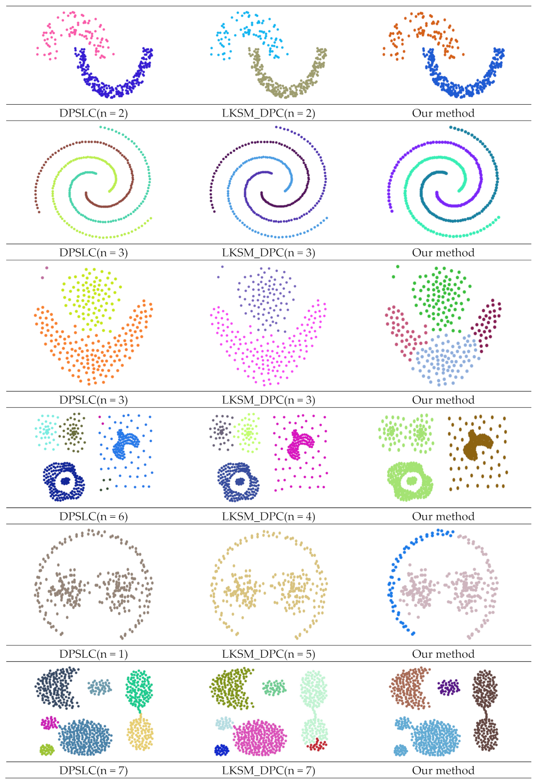
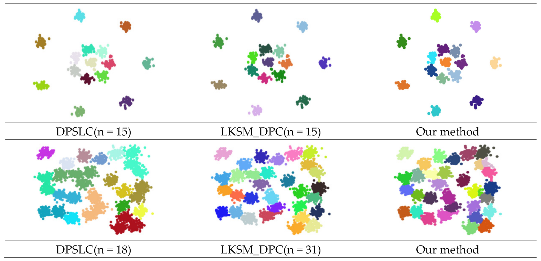
The above result proves the proposed method has the ability to detect clusters with multiple shapes and densities. In the following section, the other seven datasets are used to verify this method. We compared our method and the DPC algorithm with its extension, as well as popular density-based clustering methods, such as DBSCAN and K-means, which are shown in Figure 13 and Figure 14 and Table 1. Three clustering evaluation methods are used to access the performances of six methods. Figure 13 and Figure 14 show the cluster distribution results of the clustering methods. In Figure 13, the first column and second column show the cluster results by traditional clustering methods of K-means and DBSCAN. The third column represents the cluster results by DPC. In Figure 14, the first column and second column show the cluster results by DPSLC and LKSM_DPC. The last column shows the cluster results using our proposed clustering method. Each color stands for one cluster.
We compared our method with five clustering methods: k-means [31], DBSCAN [13], DPC [18], DPSLC [32], and LKSM_DPC [33] by using ARI [34], AMI [35] and FMI [36]. ARI (Adjusted Rand Index) is a development of RI (Rand Index), which reflects the degree of overlap between two clusters. AMI (Adjusted Mutual Information) is based on Shannon information theory, which is very popular in the clustering evaluation. FMI (Fowlkes–Mallows index) is used to measure the similarity either between two hierarchical clusters or a clustering and a benchmark classification. Some of cluster methods need set parameters in the process, such as the number of clusters. To obtain results that are the same as the benchmarks, we set the optimal parameters. In general, it is very hard to set the optimal parameters manually. According to the table, our method can accurately detect the cluster number from four datasets and the accuracy is close to the benchmark: for example, dataset (a) and the dataset mentioned in the previous section. The clustering result of the proposed method is the same as the benchmark. The same happened with dataset (b); the cluster number and accuracy are the same as the benchmark. For dataset (g) and dataset (h), the accuracy of the proposed method is nearly 100%; only a few points are not the same as the benchmark. For dataset (g), even though the cluster numbers are different, most of clusters are the same as the benchmark. It can therefore be concluded that the proposed clustering method is highly effective for detecting clusters with multiple shapes and densities. However, for dataset (c), (d), (e), and (f), there are big differences in the cluster results between the benchmark and the proposed method. The main reason is that the proposed method is more susceptible to noise. For the above four datasets, there are always a small number of points located in the space between every two clusters, making it difficult to separate one cluster from another. Compared with DPSLC and LKSM_DPC, the main advantage of the proposed method is that it does not require parameter settings that not user-friendly and require extensive experience and repeated attempts during the clustering process. The disadvantage of this method is that it considers all the data for clustering without noise filtering. Some of the data may be meaningless and should be ignored.
5. Conclusions and Future Work
This study has proposed a density-peak-based clustering method that can detect clusters of multiple shapes and densities. In this method, first, key points are detected and selected based on density and distance. Second, a hierarchical method is adopted to detect preliminary clusters by using the key points. Third, the adjacent clusters are merged gradually based on the minimum and maximum distances. Fourth, a network is constructed based on the original dataset. Lastly, the silhouette coefficient of each cluster result is calculated to identify the optimal cluster result. The proposed clustering method shows great efficiency in complex datasets that include clusters of multiple densities and shapes. For example, the detection of detailed clusters in GPS data is complicated. Hot regions with commercial buildings that attract lots of visitors may generate larger volumes of GPS data than remote regions. The advantage of this method is it does not require the manual assignment of the number of clusters and cluster center points. All the parameters that are needed in the clustering process can be automatically decided. Two improvements must be addressed in future studies. Firstly, noise is a problem that could reduce the effectiveness of this method. We plan to consider improving the noise proofing ability in complex conditions. Secondly, the time efficiency could be improved in the future work.
Author Contributions
Writing—original draft, Zhicheng Shi and Ding Ma; Project administration, Zhigang Zhao; Data curation, Xue Yan; Formal analysis, Wei Zhu. All authors have read and agreed to the published version of the manuscript.
Funding
This research was funded by the Open Fund of the Key Laboratory of Urban Land Resources Monitoring and Simulation, MNR [Grant No. KF-2018-03-016], and the National Key Research and Development Program of China [Grant No. 2018YFB2100705].
Acknowledgments
The authors would like to thank the anonymous reviewers and the editors for their valuable comments and suggestions on earlier versions of the manuscript.
Conflicts of Interest
The authors declare no conflict of interest.
References
- Bradlow, E.T.; Gangwar, M.; Kopalle, P.; Voleti, S. The role of big data and predictive analytics in retailing. J. Retail. 2017, 93, 79–95. [Google Scholar] [CrossRef] [Green Version]
- González, M.C.; Hidalgo, C.A.; Barabási, A.-L. Understanding individual human mobility patterns. Nature 2008, 453, 779–782. [Google Scholar] [CrossRef]
- Owda, A.; Balsa-Barreiro, J.; Fritsch, D. Methodology for Digital Preservation of the Cultural and Patrimonial Heritage: Generation of a 3D Model of the Church St. Peter and Paul (Calw, Germany) by Using Laser Scanning and Digital Photo-Grammetry; Emerald Publishing—Sensor Review: Bingley, UK, 2018. [Google Scholar]
- Balsa-Barreiro, J.; Lerma, L.J. A new methodology to estimate the discrete-return point density on airborne LiDAR sur-veys. Int. J. Remote Sens. 2014, 35, 1496–1510. [Google Scholar] [CrossRef]
- Balsa-Barreiro, J.; Lerma, J.L. Empirical study of variation in lidar point density over different land covers. Int. J. Remote Sens. 2014, 35, 3372–3383. [Google Scholar] [CrossRef]
- Balsa-Barreiro, J.; Avariento Vicent, J.P.; Lerma García, L.J. Airborne light detection and ranging (LiDAR) point density analysis. Sci. Res. Essays 2012, 7, 3010–3019. [Google Scholar] [CrossRef]
- Han, J.; Pei, J.; Kamber, M. Data Mining: Concepts and Techniques; Elsevier: Amsterdam, The Netherlands, 2011. [Google Scholar]
- Raykov, Y.P.; Boukouvalas, A.; Baig, F.; Little, M.A. What to do when k-means clustering fails: A simple yet principled alternative Algorithm. PLoS ONE 2016, 11, e0162259. [Google Scholar] [CrossRef] [Green Version]
- Park, H.-S.; Jun, C.-H. A simple and fast algorithm for K-medoids clustering. Expert Syst. Appl. 2009, 36, 3336–3341. [Google Scholar] [CrossRef]
- Zhang, T.; Ramakrishnan, R.; Livny, M. BIRCH: An efficient data clustering method for very large databases. ACM Sigmod Rec. 1996, 25, 103–114. [Google Scholar] [CrossRef]
- Guha, S.; Rastogi, R.; Shim, K. Cure: An efficient clustering algorithm for large databases. Inf. Syst. 2001, 26, 35–58. [Google Scholar] [CrossRef]
- Karypis, G.; Han, E.-H.; Kumar, V. Chameleon: Hierarchical clustering using dynamic modeling. Computer 1999, 32, 68–75. [Google Scholar] [CrossRef] [Green Version]
- Ester, M.; Kriegel, H.P.; Sander, J.; Xu, X. A density-based algorithm for discovering clusters in large spatial databases with noise. In Proceedings of the 2nd International Conference on Knowledge Discovery and Data Mining KDD-96, Portland, OR, USA, 2–4 August 1996; pp. 226–231. [Google Scholar]
- Ankerst, M.; Breunig, M.M.; Kriegel, H.-P.; Sander, J. OPTICS: Ordering points to identify the clustering structure. ACM Sigmod Rec. 1999, 28, 49–60. [Google Scholar] [CrossRef]
- Hinneburg, A.; Gabriel, H.-H. DENCLUE 2.0: Fast clustering based on kernel density estimation. In OpenMP in the Era of Low Power Devices and Accelerators; Springer Science and Business Media LLC.: Berlin/Heidelberg, Germany, 2007; pp. 70–80. [Google Scholar]
- Wang, W.; Yang, J.; Muntz, R. STING: A statistical information grid approach to spatial data mining. VLDB 1997, 97, 186–195. [Google Scholar]
- Uncu, Ö.; Gruver, W.A.; Kotak, D.B.; Sabaz, D.; Alibhai, Z.; Ng, C. GRIDBSCAN: GRId density-based spatial clustering of applications with noise. In Proceedings of the 2006 IEEE International Conference on Systems, Man and Cybernetics, Taipei, Taiwan, 8–11 October 2006; 2006; Volume 4, pp. 2976–2981. [Google Scholar]
- Rodriguez, A.; Laio, A. Clustering by fast search and find of density peaks. Science 2014, 344, 1492–1496. [Google Scholar] [CrossRef] [PubMed] [Green Version]
- Anders, K.-H.; Sester, M. Parameter-free cluster detection in spatial databases and its application to typification. Int. Arch. Photogramm. Remote Sens. 2000, 33, 75–83. [Google Scholar]
- Ding, J.; He, X.; Yuan, J.; Jiang, B. Automatic clustering based on density peak detection using generalized extreme value distribution. Soft Comput. 2018, 22, 2777–2796. [Google Scholar] [CrossRef]
- Liu, Y.; Ma, Z.; Yu, F. Adaptive density peak clustering based on K-nearest neighbors with aggregating strategy. Knowl.-Based Syst. 2017, 133, 208–220. [Google Scholar]
- Xie, J.; Gao, H.; Xie, W.; Liu, X.; Grant, P.W. Robust clustering by detecting density peaks and assigning points based on fuzzy weighted K-nearest neighbors. Inf. Sci. 2016, 354, 19–40. [Google Scholar] [CrossRef]
- Du, M.; Ding, S.; Jia, H. Study on density peaks clustering based on k-nearest neighbors and principal component analysis. Knowl.-Based Syst. 2016, 99, 135–145. [Google Scholar] [CrossRef]
- Jinyin, C.; Xiang, L.; Haibing, Z.; Xintong, B. A novel cluster center fast determination clustering algorithm. Appl. Soft Comput. 2017, 57, 539–555. [Google Scholar] [CrossRef]
- Ruan, S.; Mehmood, R.; Daud, A.; Dawood, H.; Alowibdi, J.S. An adaptive method for clustering by fast search-and-find of density peaks: Adaptive-dp. In Proceedings of the 26th International Conference on World Wide Web Companion, Perth, Australia, 3–7 April 2017; pp. 119–127. [Google Scholar]
- Wang, G.; Song, Q. Automatic clustering via outward statistical testing on density metrics. IEEE Trans. Knowl. Data Eng. 2016, 28, 1971–1985. [Google Scholar] [CrossRef]
- Xu, J.; Wang, G.; Deng, W. DenPEHC: Density peak based efficient hierarchical clustering. Inf. Sci. 2016, 373, 200–218. [Google Scholar] [CrossRef]
- Wang, M.; Zuo, W.; Wang, Y. An improved density peaks-based clustering method for social circle discovery in social networks. Neurocomputing 2016, 179, 219–227. [Google Scholar] [CrossRef]
- Parmar, M.; Wang, D.; Zhang, X.; Tan, A.H.; Miao, C.; Jiang, J.; Zhou, Y. REDPC: A residual error-based density peak clustering algorithm. Neurocomputing 2019, 348, 82–96. [Google Scholar] [CrossRef]
- Rousseeuw, P.J. Silhouettes: A graphical aid to the interpretation and validation of cluster analysis. J. Comput. Appl. Math. 1987, 20, 53–65. [Google Scholar] [CrossRef] [Green Version]
- MacQueen, J. Some methods for classification and analysis of multivariate observations. In Proceedings of the Fifth Berkeley Symposium on Mathematical Statistics and Probability, Berkeley, CA, USA, 21 June–18 July 1965; Volume 1, pp. 281–297. [Google Scholar]
- Lin, J.-L.; Kuo, J.-C.; Chuang, H.-W. Improving density peak clustering by automatic peak selection and single linkage clustering. Symmetry 2020, 12, 1168. [Google Scholar] [CrossRef]
- Ren, C.; Sun, L.; Yu, Y.; Wu, Q. Effective density peaks clustering algorithm based on the layered k-nearest neighbors and subcluster merging. IEEE Access 2020, 8, 123449–123468. [Google Scholar] [CrossRef]
- Hubert, L.; Arabie, P. Comparing partitions. J. Classif. 1985, 2, 193–218. [Google Scholar] [CrossRef]
- Lazarenko, D.; Bonald, T. Pairwise adjusted mutual information. arXiv 2021, arXiv:2103.12641. [Google Scholar]
- Campello, R. A fuzzy extension of the Rand index and other related indexes for clustering and classification assessment. Pattern Recognit. Lett. 2007, 28, 833–841. [Google Scholar] [CrossRef]
Figure 1.
Logical flow of the proposed clustering method.

Figure 2.
Categories of points distribution.
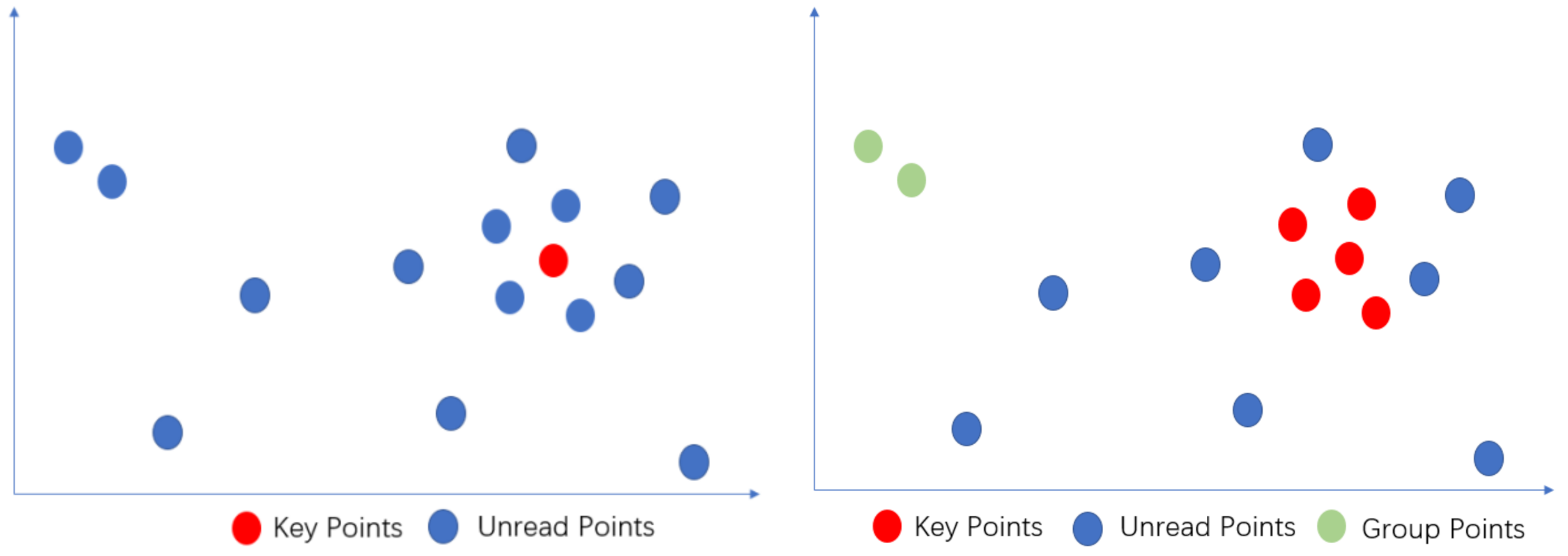
Figure 3.
Example dataset distribution and calculation result (a) distribution of dataset; (b) distribution of local density and distance; and (c) product result of local density and distance.
Figure 3.
Example dataset distribution and calculation result (a) distribution of dataset; (b) distribution of local density and distance; and (c) product result of local density and distance.

Figure 4.
Key points detection of dataset with multiple shapes and densities (a) distribution of the dataset; (b) two core points are selected; (c) the distribution of two core points in the dataset; (d) three core points are selected; (e) the distribution of three core points in the dataset.
Figure 4.
Key points detection of dataset with multiple shapes and densities (a) distribution of the dataset; (b) two core points are selected; (c) the distribution of two core points in the dataset; (d) three core points are selected; (e) the distribution of three core points in the dataset.
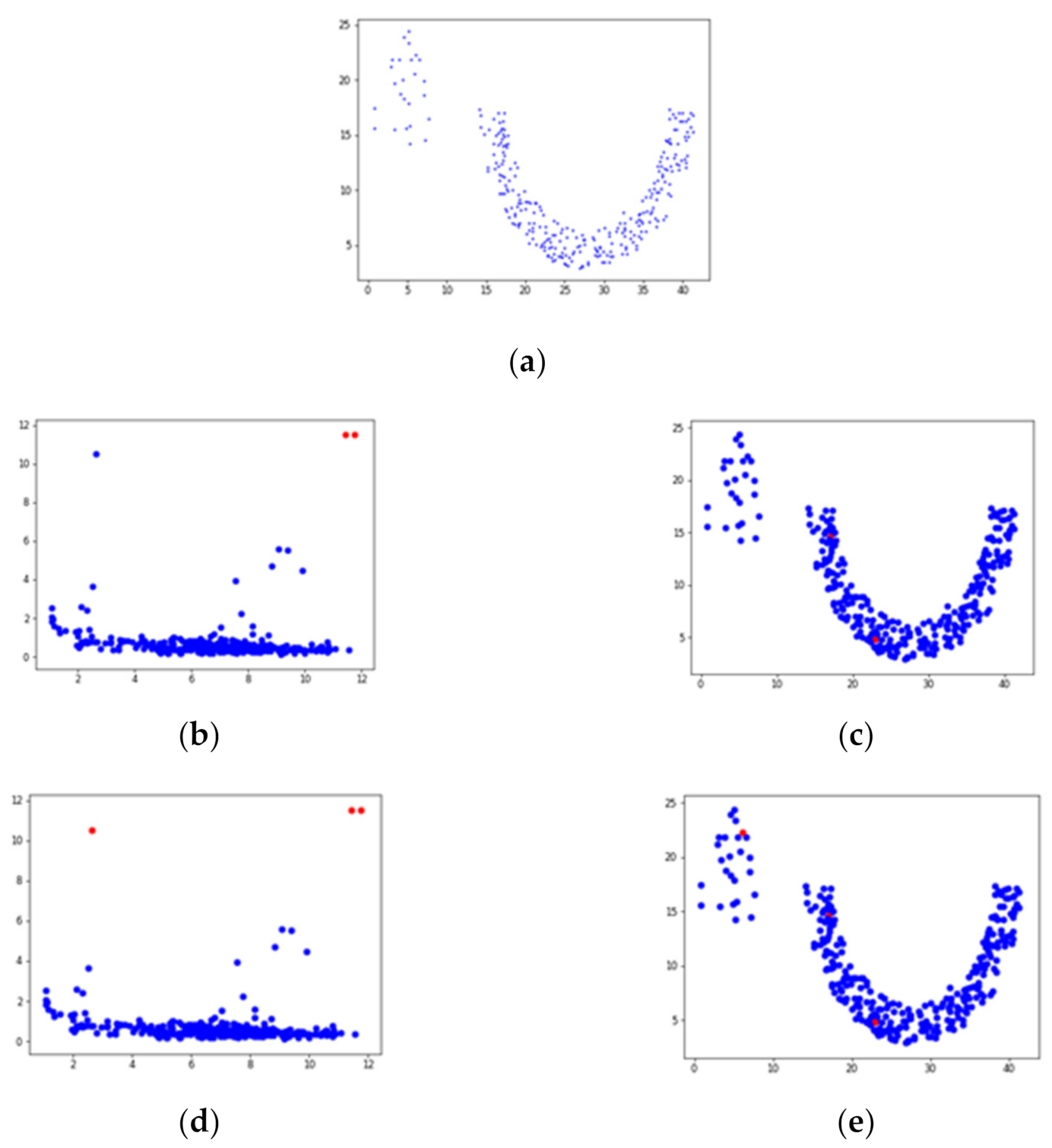
Figure 5.
Logical flow of detect preliminary clusters.
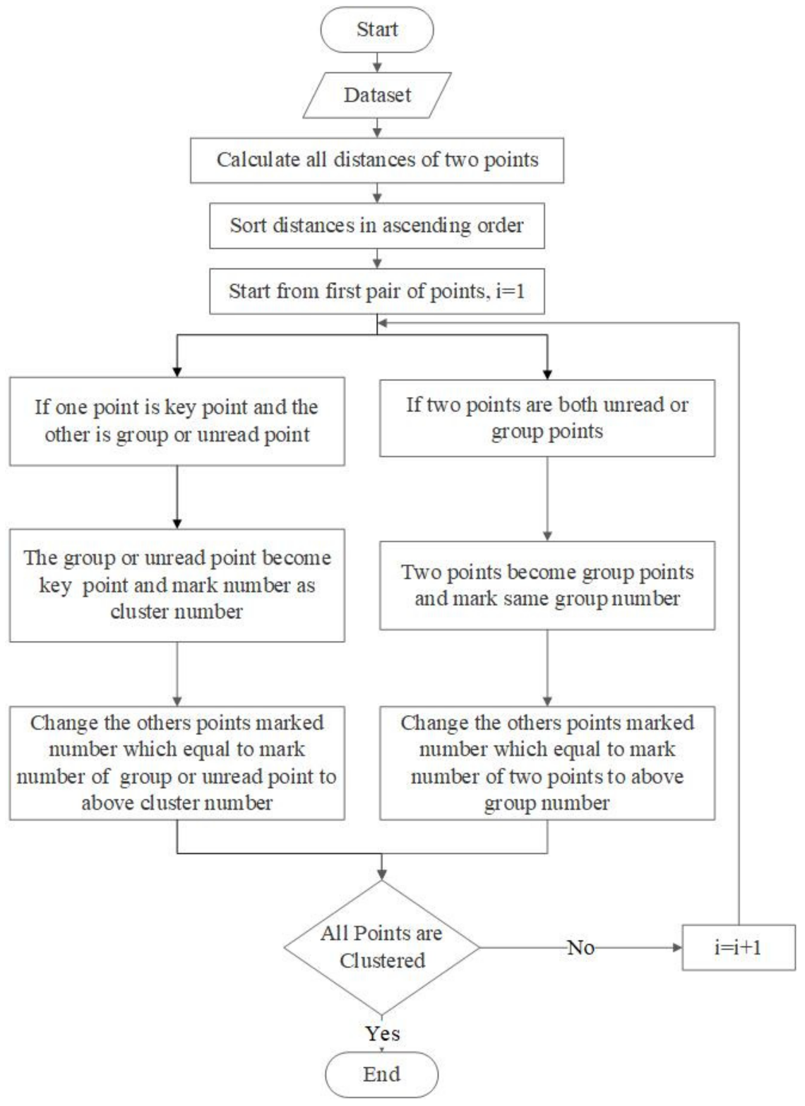
Figure 6.
Examples of merging process (a) the process of merging Cluster B and C; (b) the process of merging Cluster A and B.
Figure 6.
Examples of merging process (a) the process of merging Cluster B and C; (b) the process of merging Cluster A and B.
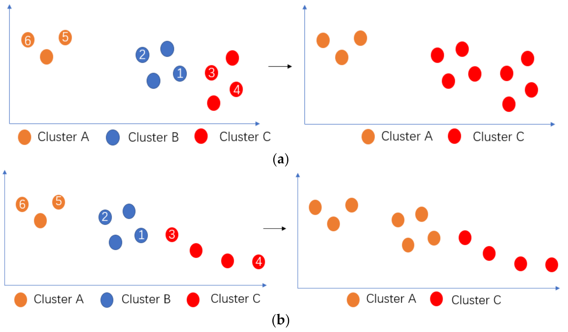
Figure 7.
Dataset distribution.

Figure 8.
Calculate and select key points: (a) the distribution of product results; (b) key points’ selection result.
Figure 8.
Calculate and select key points: (a) the distribution of product results; (b) key points’ selection result.
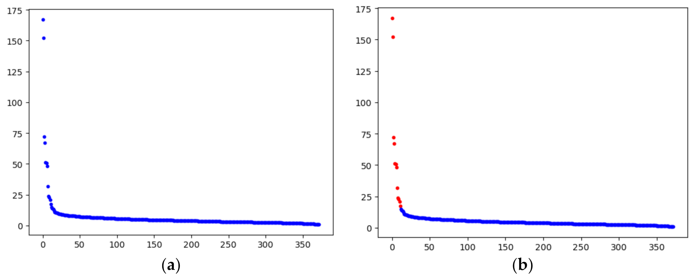
Figure 9.
Detected preliminary clusters: (a) key point distribution in dataset; (b) cluster distribution of detected preliminary result.
Figure 9.
Detected preliminary clusters: (a) key point distribution in dataset; (b) cluster distribution of detected preliminary result.
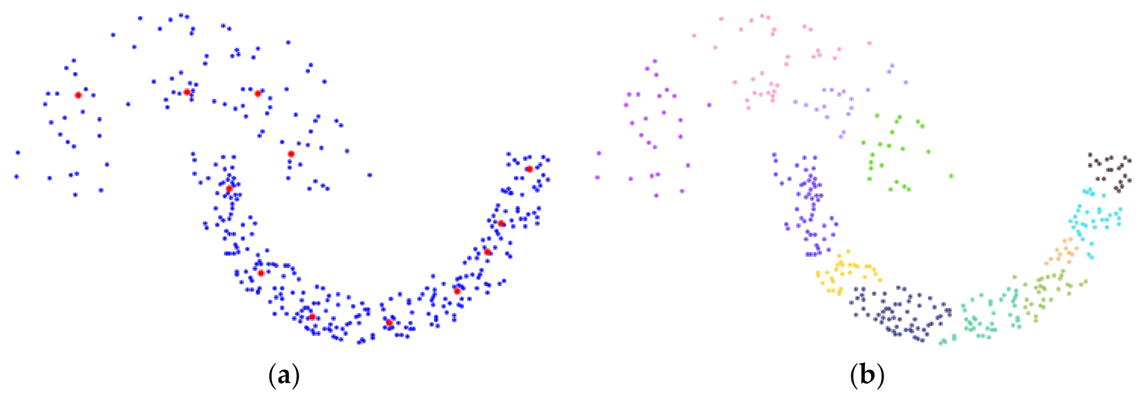
Figure 10.
Network construction.
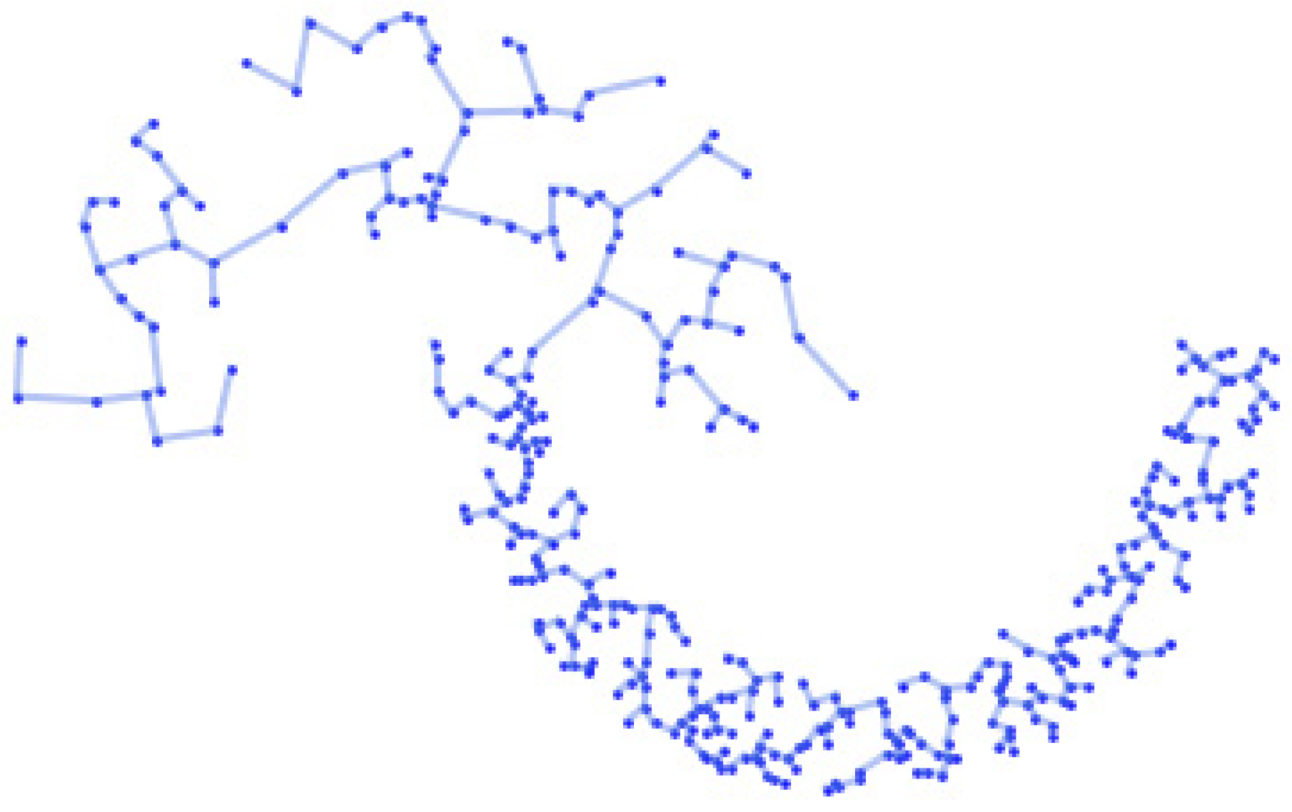
Figure 11.
Silhouette coefficient results.
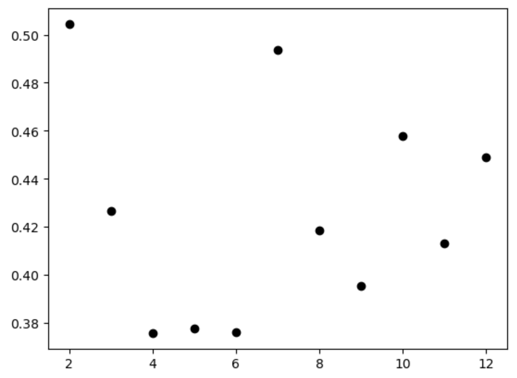
Figure 12.
The optimal clusters distribution.
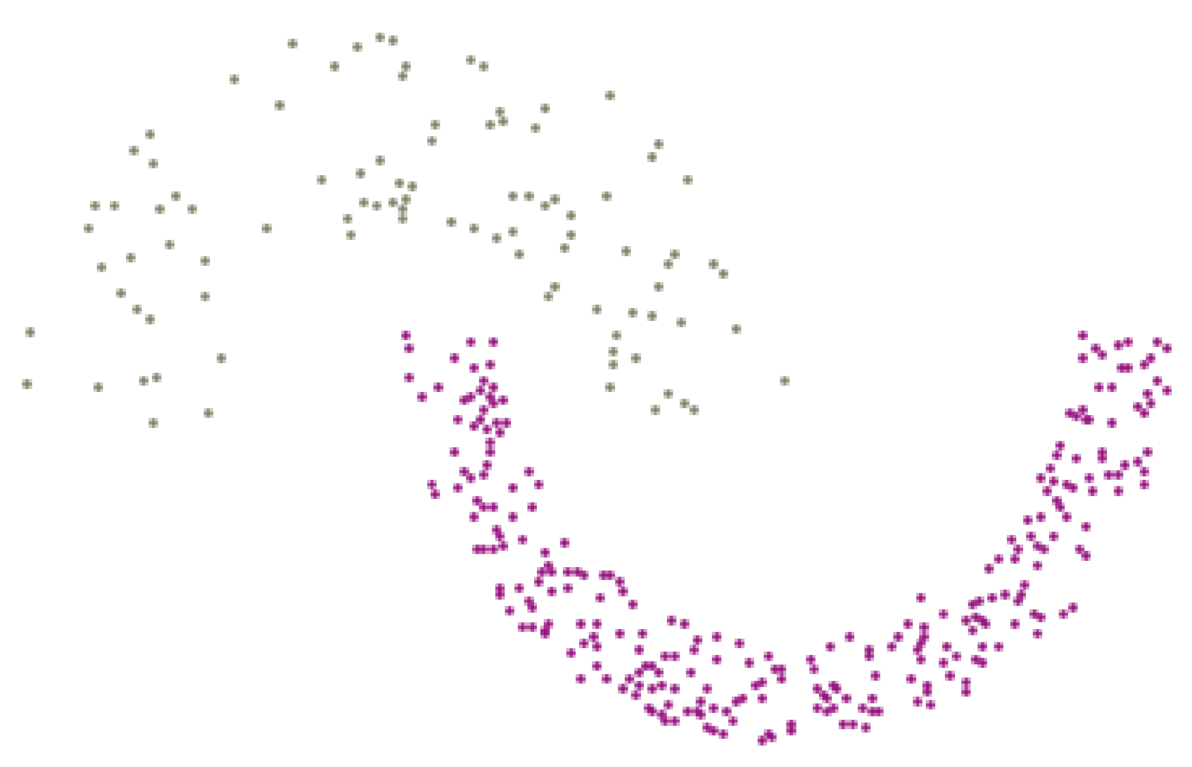
Figure 13.
Clustering results by K-means, DBSCAN, and DPC of dataset a–h.
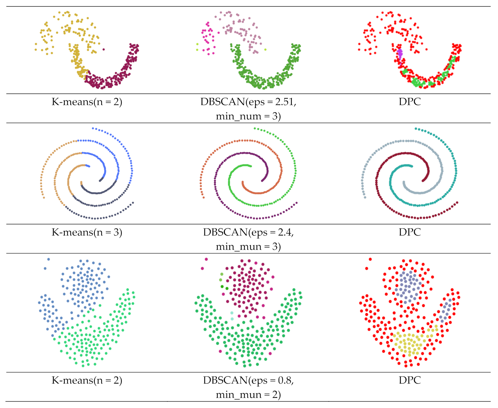
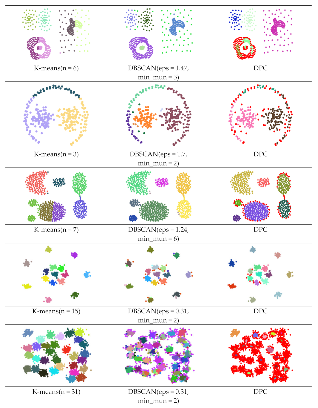
Figure 14.
Clustering results by DPSLC, LKSM_DPC and proposed method of dataset a–h.

Table 1.
Clustering evaluations on dataset a–h.
| Dataset | Method | ARI | AMI | FMI |
|---|---|---|---|---|
| Dataset (a) | K-means | 0.318 | 0.364 | 0.698 |
| DBSCAN | 0.941 | 0.864 | 0.977 | |
| DPC | −0.051 | 0.177 | 0.550 | |
| DPSLC | 1.000 | 1.000 | 1.000 | |
| LKSM_DPC | 1.000 | 1.000 | 1.000 | |
| Our method | 1.000 | 1.000 | 1.000 | |
| Dataset (b) | K-means | −0.006 | −0.005 | 0.328 |
| DBSCAN | 1.000 | 1.000 | 1.000 | |
| DPC | 1.000 | 1.000 | 1.000 | |
| DPSLC | 1.000 | 1.000 | 1.000 | |
| LKSM_DPC | 1.000 | 1.000 | 1.000 | |
| Our method | 1.000 | 1.000 | 1.000 | |
| Dataset (c) | K-means | 0.453 | 0.397 | 0.736 |
| DBSCAN | 0.878 | 0.791 | 0.941 | |
| DPC | 0.080 | 0.171 | 0.551 | |
| DPSLC | 0.988 | 0.970 | 0.994 | |
| LKSM_DPC | 1.000 | 1.000 | 1.000 | |
| Our method | 0.521 | 0.668 | 0.735 | |
| Dataset (d) | K-means | 0.538 | 0.713 | 0.642 |
| DBSCAN | 0.976 | 0.950 | 0.982 | |
| DPC | 0.578 | 0.754 | 0.680 | |
| DPSLC | 0.788 | 0.846 | 0.856 | |
| LKSM_DPC | 0.783 | 0.858 | 0.855 | |
| Our method | 0.437 | 0.585 | 0.676 | |
| Dataset (e) | K-means | 0.461 | 0.543 | 0.662 |
| DBSCAN | 0.529 | 0.640 | 0.687 | |
| DPC | 0.438 | 0.455 | 0.622 | |
| DPSLC | 0.000 | 0.000 | 0.577 | |
| LKSM_DPC | 0.000 | 0.000 | 0.000 | |
| Our method | 0.126 | 0.290 | 0.554 | |
| Dataset (f) | K-means | 0.762 | 0.878 | 0.816 |
| DBSCAN | 0.980 | 0.971 | 0.984 | |
| DPC | 0.851 | 0.876 | 0.884 | |
| DPSLC | 0.998 | 0.996 | 0.998 | |
| LKSM_DPC | 0.890 | 0.924 | 0.917 | |
| Our method | 0.734 | 0.835 | 0.819 | |
| Dataset (g) | K-means | 0.993 | 0.994 | 0.993 |
| DBSCAN | 0.921 | 0.936 | 0.927 | |
| DPC | 0.975 | 0.980 | 0.976 | |
| DPSLC | 0.993 | 0.994 | 0.993 | |
| LKSM_DPC | 0.986 | 0.989 | 0.987 | |
| Our method | 0.986 | 0.989 | 0.987 | |
| Dataset (h) | K-means | 0.953 | 0.966 | 0.955 |
| DBSCAN | 0.550 | 0.768 | 0.565 | |
| DPC | 0.031 | 0.445 | 0.176 | |
| DPSLC | 0.585 | 0.869 | 0.653 | |
| LKSM_DPC | 0.935 | 0.956 | 0.938 | |
| Our method | 0.928 | 0.951 | 0.930 |
Publisher’s Note: MDPI stays neutral with regard to jurisdictional claims in published maps and institutional affiliations. |
© 2021 by the authors. Licensee MDPI, Basel, Switzerland. This article is an open access article distributed under the terms and conditions of the Creative Commons Attribution (CC BY) license (https://creativecommons.org/licenses/by/4.0/).
Share and Cite
MDPI and ACS Style
Shi, Z.; Ma, D.; Yan, X.; Zhu, W.; Zhao, Z. A Density-Peak-Based Clustering Method for Multiple Densities Dataset. ISPRS Int. J. Geo-Inf. 2021, 10, 589. https://doi.org/10.3390/ijgi10090589
AMA Style
Shi Z, Ma D, Yan X, Zhu W, Zhao Z. A Density-Peak-Based Clustering Method for Multiple Densities Dataset. ISPRS International Journal of Geo-Information. 2021; 10(9):589. https://doi.org/10.3390/ijgi10090589
Chicago/Turabian StyleShi, Zhicheng, Ding Ma, Xue Yan, Wei Zhu, and Zhigang Zhao. 2021. "A Density-Peak-Based Clustering Method for Multiple Densities Dataset" ISPRS International Journal of Geo-Information 10, no. 9: 589. https://doi.org/10.3390/ijgi10090589
Note that from the first issue of 2016, this journal uses article numbers instead of page numbers. See further details here.