
Sentinel 2 Time Series Analysis with 3D Feature Pyramid Network and Time Domain Class Activation Intervals for Crop Mapping


Abstract
:
1. Introduction
- We propose a new semantic segmentation model suitable for remote sensing time series.
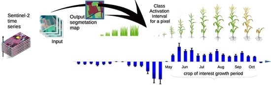
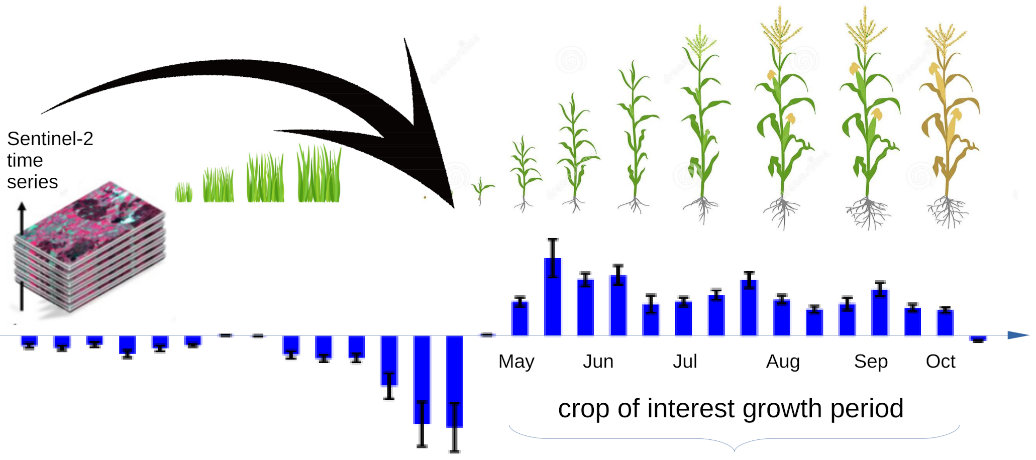
- We add to the proposed CNN a mechanism that allows visualizing the time interval of the time series that contribute to the determination of the class for each pixel.
- We exceed by about the state of the art on a public dataset with satellite time series.
2. Proposed Method
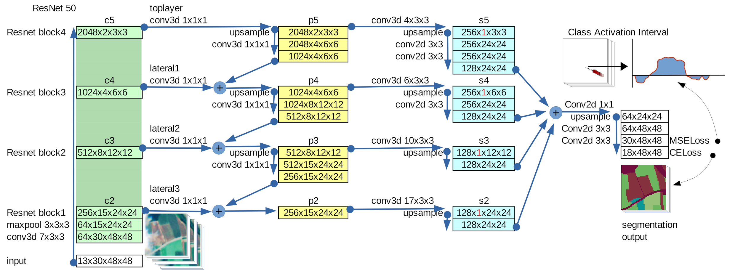
2.1. (3+2)D Features Pyramid Network
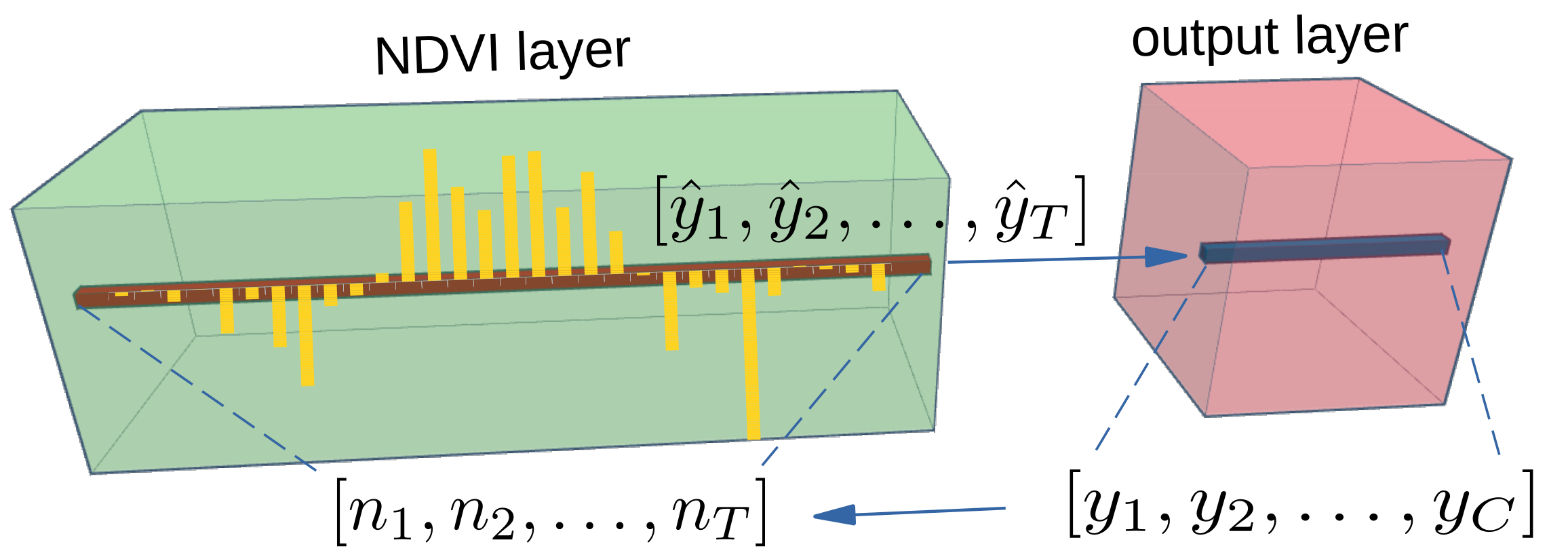
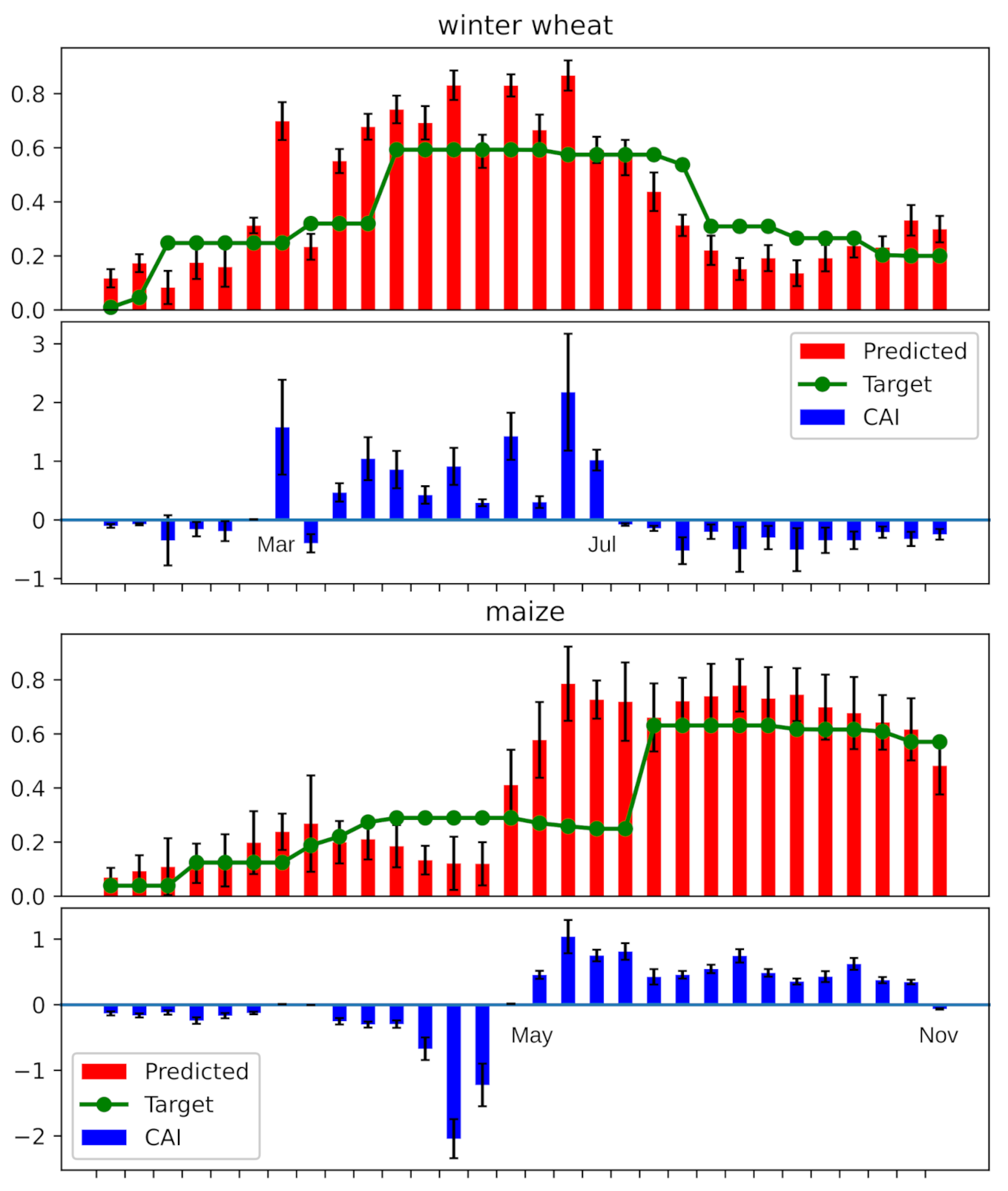
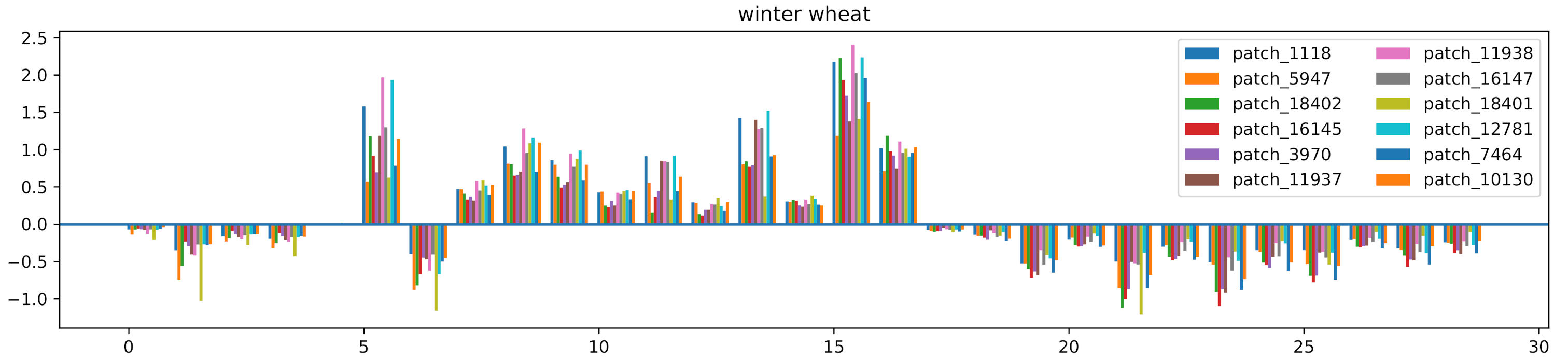
2.2. Class Activation Intervals
3. Dataset
4. Experiments
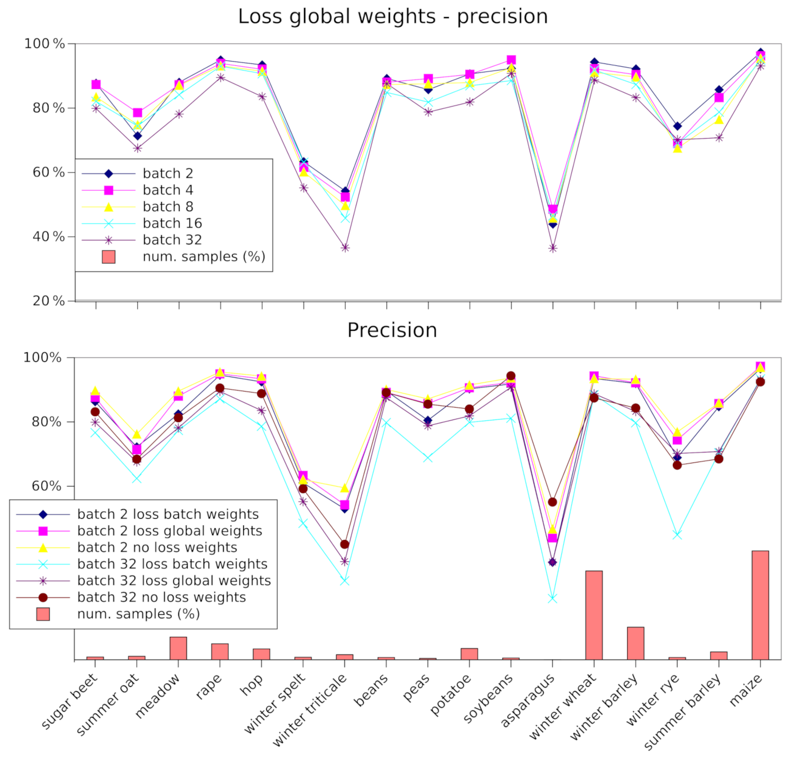
4.1. Class Imbalance Experiments
4.2. Comparisons
4.3. Experiments on CAI and Ablation Study
5. Conclusions
Author Contributions
Funding
Institutional Review Board Statement
Informed Consent Statement
Conflicts of Interest
References
- Sochor, J.; Herout, A.; Havel, J. Boxcars: 3d boxes as cnn input for improved fine-grained vehicle recognition. In Proceedings of the IEEE Conference on Computer Vision and Pattern Recognition, Las Vegas, NV, USA, 27–30 June 2016; pp. 3006–3015. [Google Scholar]
- Liu, J.; Cao, L.; Akin, O.; Tian, Y. Accurate and Robust Pulmonary Nodule Detection by 3D Feature Pyramid Network with Self-supervised Feature Learning. arXiv 2019, arXiv:1907.11704. [Google Scholar]
- Simonyan, K.; Zisserman, A. Two-stream convolutional networks for action recognition in videos. Adv. Neural Inf. Process. Syst. 2014, 27, 568–576. [Google Scholar]
- Feichtenhofer, C.; Pinz, A.; Zisserman, A. Convolutional two-stream network fusion for video action recognition. In Proceedings of the IEEE Conference on Computer Vision and Pattern Recognition, Las Vegas, NV, USA, 27–30 June 2016; pp. 1933–1941. [Google Scholar]
- Burceanu, E.; Leordeanu, M. A 3d convolutional approach to spectral object segmentation in space and time. In Proceedings of the Twenty-Ninth International Joint Conference on Artificial Intelligence, IJCAI, Vienna, Austria, 23–29 July 2020; pp. 495–501. [Google Scholar]
- Hara, K.; Kataoka, H.; Satoh, Y. Can spatiotemporal 3d cnns retrace the history of 2d cnns and imagenet? In Proceedings of the IEEE Conference on Computer Vision and Pattern Recognition, Salt Lake City, UT, USA, 18–23 June 2018; pp. 6546–6555. [Google Scholar]
- Qiu, Z.; Yao, T.; Mei, T. Learning spatio-temporal representation with pseudo-3d residual networks. In Proceedings of the IEEE International Conference on Computer Vision, Venice, Italy, 22–29 October 2017; pp. 5533–5541. [Google Scholar]
- Tran, D.; Wang, H.; Torresani, L.; Ray, J.; LeCun, Y.; Paluri, M. A closer look at spatiotemporal convolutions for action recognition. In Proceedings of the IEEE Conference on Computer Vision and Pattern Recognition, Salt Lake City, UT, USA, 18–23 June 2018; pp. 6450–6459. [Google Scholar]
- Sentinel Dataflow from Copernicus Program. 2021. Available online: https://www.copernicus.eu/en (accessed on 11 July 2021).
- Lin, T.Y.; Dollár, P.; Girshick, R.; He, K.; Hariharan, B.; Belongie, S. Feature pyramid networks for object detection. In Proceedings of the IEEE Conference on Computer Vision and Pattern Recognition, Honolulu, HI, USA, 21–26 July 2017; pp. 2117–2125. [Google Scholar]
- Seferbekov, S.S.; Iglovikov, V.; Buslaev, A.; Shvets, A. Feature Pyramid Network for Multi-Class Land Segmentation. In Proceedings of the IEEE/CVF Conference on Computer Vision and Pattern Recognition Workshops (CVPRW), Salt Lake City, UT, USA, 2018; pp. 272–275. [Google Scholar]
- Ronneberger, O.; Fischer, P.; Brox, T. U-net: Convolutional networks for biomedical image segmentation. In International Conference on Medical Image Computing and Computer-Assisted Intervention; Springer: Berlin/Heidelberg, Germany, 2015; pp. 234–241. [Google Scholar]
- Isensee, F.; Jäger, P.F.; Kohl, S.A.; Petersen, J.; Maier-Hein, K.H. Automated design of deep learning methods for biomedical image segmentation. arXiv 2019, arXiv:1904.08128. [Google Scholar]
- Zhou, B.; Khosla, A.; Lapedriza, A.; Oliva, A.; Torralba, A. Learning deep features for discriminative localization. In Proceedings of the IEEE Conference on Computer Vision and Pattern Recognition, Las Vegas, NV, USA, 27–30 June 2016; pp. 2921–2929. [Google Scholar]
- Zhou, B.; Khosla, A.; Lapedriza, A.; Oliva, A.; Torralba, A. Object detectors emerge in deep scene cnns. arXiv 2014, arXiv:1412.6856. [Google Scholar]
- Selvaraju, R.R.; Cogswell, M.; Das, A.; Vedantam, R.; Parikh, D.; Batra, D. Grad-cam: Visual explanations from deep networks via gradient-based localization. In Proceedings of the IEEE International Conference on Computer Vision, Venice, Italy, 22–29 October 2017; pp. 618–626. [Google Scholar]
- Kirillov, A.; Girshick, R.; He, K.; Dollár, P. Panoptic feature pyramid networks. In Proceedings of the IEEE Conference on Computer Vision and Pattern Recognition, Long Beach, CA, USA, 15–20 June 2019; pp. 6399–6408. [Google Scholar]
- Zhu, L.; Deng, Z.; Hu, X.; Fu, C.W.; Xu, X.; Qin, J.; Heng, P.A. Bidirectional feature pyramid network with recurrent attention residual modules for shadow detection. In Proceedings of the European Conference on Computer Vision (ECCV), Munich, Germany, 8–14 September 2018; pp. 121–136. [Google Scholar]
- Rousel, J.; Haas, R.; Schell, J.; Deering, D. Monitoring vegetation systems in the great plains with ERTS. In Proceedings of the Third Earth Resources Technology Satellite—1 Symposium; NASA: Washington, DC, USA, 1974; pp. 309–317. [Google Scholar]
- Rußwurm, M.; Körner, M. Multi-temporal land cover classification with sequential recurrent encoders. ISPRS Int. J. Geo-Inf. 2018, 7, 129. [Google Scholar] [CrossRef] [Green Version]
- Rußwurm, M.K.M. Munich Dataset. 2018. Available online: https://github.com/tum-lmf/mtlcc-pytorch (accessed on 11 January 2021).
- McHugh, M.L. Interrater reliability: The kappa statistic. Biochem. Medica Biochem. Medica 2012, 22, 276–282. [Google Scholar] [CrossRef]
- Robbins, H.; Monro, S. A stochastic approximation method. Ann. Math. Stat. 1951, 22, 400–407. [Google Scholar] [CrossRef]
- Gallo, I.; La Grassa, R.; Landro, N.; Boschetti, M. Pytorch Source Code for the Model Proposed in This Paper. 2021. Available online: https://gitlab.com/ignazio.gallo/sentinel-2-time-series-with-3d-fpn-and-time-domain-cai (accessed on 11 July 2021).
- Cui, Y.; Jia, M.; Lin, T.Y.; Song, Y.; Belongie, S. Class-Balanced Loss Based on Effective Number of Samples. In Proceedings of the IEEE Conference on Computer Vision and Pattern Recognition, Long Beach, CA, USA, 15–20 June 2019. [Google Scholar]


| [20] | Our (Eval Set) | Our (Test Set) | ||||||||||
|---|---|---|---|---|---|---|---|---|---|---|---|---|
| P | R | F1 | #pix. | P | R | F1 | #pix. | P | R | F1 | #pix. | |
| sugar beet | 91.90 | 78.05 | 84.40 | 59k | 90.95 | 93.66 | 92.29 | 19k | 96.37 | 89.65 | 92.88 | 33k |
| oat | 74.95 | 65.30 | 69.55 | 36k | 79.17 | 68.13 | 73.23 | 23k | 83.28 | 69.88 | 75.99 | 30k |
| meadow | 89.45 | 85.35 | 87.35 | 233k | 89.51 | 87.45 | 88.47 | 149k | 93.27 | 89.53 | 91.36 | 167k |
| rapeseed | 95.80 | 92.95 | 94.35 | 125k | 95.98 | 97.64 | 96.81 | 105k | 95.99 | 97.99 | 96.98 | 92k |
| hop | 94.45 | 81.10 | 87.20 | 51k | 95.12 | 93.26 | 94.18 | 71k | 95.55 | 93.94 | 94.74 | 39k |
| spelt | 65.20 | 63.90 | 61.60 | 38k | 66.39 | 51.12 | 57.76 | 17k | 68.02 | 59.69 | 63.58 | 23k |
| triticale | 65.90 | 56.45 | 60.75 | 65k | 57.24 | 36.03 | 44.22 | 34k | 58.20 | 44.59 | 50.49 | 41k |
| beans | 92.60 | 75.15 | 82.40 | 27k | 91.40 | 79.03 | 84.77 | 15k | 95.26 | 88.63 | 91.82 | 19k |
| peas | 77.05 | 56.10 | 64.85 | 9k | 87.07 | 65.26 | 74.61 | 9k | 81.21 | 83.77 | 82.47 | 6k |
| potato | 93.05 | 81.00 | 86.30 | 126k | 91.37 | 91.58 | 91.48 | 74k | 90.94 | 92.32 | 91.63 | 84k |
| soybeans | 86.80 | 79.75 | 82.75 | 21k | 96.05 | 84.33 | 89.81 | 12k | 96.96 | 81.82 | 88.75 | 14k |
| asparagus | 85.40 | 78.15 | 81.60 | 20k | 70.86 | 92.34 | 80.19 | 1k | 95.72 | 84.98 | 90.03 | 14k |
| wheat | 88.90 | 94.05 | 91.40 | 806k | 93.85 | 96.68 | 95.24 | 582k | 92.66 | 95.74 | 94.17 | 531k |
| winter barley | 93.85 | 89.75 | 91.70 | 258k | 93.52 | 95.01 | 94.26 | 214k | 93.19 | 95.28 | 94.23 | 170k |
| rye | 81.15 | 54.45 | 64.60 | 43k | 83.58 | 57.51 | 68.14 | 15k | 82.36 | 59.14 | 68.85 | 25k |
| summer barley | 82.70 | 85.95 | 84.15 | 73k | 84.94 | 87.71 | 86.30 | 52k | 84.60 | 89.54 | 87.00 | 52k |
| maize | 91.95 | 96.55 | 94.20 | 919k | 96.74 | 98.03 | 97.38 | 713k | 96.44 | 98.19 | 97.31 | 604k |
| weighted avg. | 89.70 | 89.60 | 89.40 | 93.22 | 93.55 | 93.39 | 92.94 | 92.68 | 92.81 | |||
| Overall Accuracy | 89.60 | Overall Accuracy | 93.55 | Overall Accuracy | 92.94 | |||||||
| Overall Kappa | 0.87 | Overall Kappa | 0.92 | Overall Kappa | 0.91 | |||||||
| Weight | Batch | OA | Kappa | w. R | w. P | w. F1 |
|---|---|---|---|---|---|---|
| batch | 2 | 91.98 | 0.920 | 91.98 | 91.78 | 91.82 |
| batch | 4 | 91.64 | 0.894 | 91.64 | 91.18 | 91.30 |
| batch | 8 | 90.55 | 0.879 | 90.55 | 89.84 | 90.00 |
| batch | 16 | 89.39 | 0.865 | 89.39 | 89.09 | 89.14 |
| batch | 32 | 85.82 | 0.820 | 85.82 | 85.16 | 85.31 |
| global | 2 | 93.17 | 0.913 | 93.17 | 92.89 | 92.96 |
| global | 4 | 92.10 | 0.899 | 92.10 | 91.54 | 91.62 |
| global | 8 | 91.06 | 0.886 | 91.06 | 90.40 | 90.43 |
| global | 16 | 90.34 | 0.877 | 90.34 | 89.86 | 89.97 |
| global | 32 | 87.22 | 0.837 | 87.22 | 86.48 | 86.59 |
| no | 2 | 93.71 | 0.920 | 93.71 | 93.41 | 93.56 |
| no | 4 | 92.33 | 0.902 | 92.33 | 91.71 | 91.73 |
| no | 8 | 91.21 | 0.887 | 91.21 | 90.35 | 90.44 |
| no | 16 | 90.54 | 0.879 | 90.54 | 90.00 | 90.07 |
| no | 32 | 87.56 | 0.840 | 87.56 | 86.69 | 86.54 |
| Backbone | acc. | MSE Loss |
|---|---|---|
| ResNet101 | 93.48% | no |
| ResNet101 | 93.71% | yes |
| ResNet50 | 93.62% | yes |
| ResNet34 | 92.19% | yes |
| ResNet18 | 91.57% | yes |
| ResNet10 | 91.37% | yes |
Publisher’s Note: MDPI stays neutral with regard to jurisdictional claims in published maps and institutional affiliations. |
© 2021 by the authors. Licensee MDPI, Basel, Switzerland. This article is an open access article distributed under the terms and conditions of the Creative Commons Attribution (CC BY) license (https://creativecommons.org/licenses/by/4.0/).
Share and Cite
Gallo, I.; La Grassa, R.; Landro, N.; Boschetti, M. Sentinel 2 Time Series Analysis with 3D Feature Pyramid Network and Time Domain Class Activation Intervals for Crop Mapping. ISPRS Int. J. Geo-Inf. 2021, 10, 483. https://doi.org/10.3390/ijgi10070483
Gallo I, La Grassa R, Landro N, Boschetti M. Sentinel 2 Time Series Analysis with 3D Feature Pyramid Network and Time Domain Class Activation Intervals for Crop Mapping. ISPRS International Journal of Geo-Information. 2021; 10(7):483. https://doi.org/10.3390/ijgi10070483
Chicago/Turabian StyleGallo, Ignazio, Riccardo La Grassa, Nicola Landro, and Mirco Boschetti. 2021. "Sentinel 2 Time Series Analysis with 3D Feature Pyramid Network and Time Domain Class Activation Intervals for Crop Mapping" ISPRS International Journal of Geo-Information 10, no. 7: 483. https://doi.org/10.3390/ijgi10070483
APA StyleGallo, I., La Grassa, R., Landro, N., & Boschetti, M. (2021). Sentinel 2 Time Series Analysis with 3D Feature Pyramid Network and Time Domain Class Activation Intervals for Crop Mapping. ISPRS International Journal of Geo-Information, 10(7), 483. https://doi.org/10.3390/ijgi10070483